Which cubic spline should one use?

WHICH CUBIC SPLINE SHOULD ONE USE?

by

R.K. Beatson and E. Chacko

Department of Mathematics, University of Canterbury, Christchurch, New Zealand.

Which cubic spline should one use?

R.K. Beatson and E. Chacko*

November 30, 1990

Abstract

The aim of this paper is to provide a quantitative comparison of eight different 01 _{and 0}2 _{cubic spline interpolation schemes. The 0}1 _schemes discussed are local while the 02 _{ones are global.}

In practice cubic splines are often used when the smoothness of the function being interpolated/approximated is unknown. Also it is often necessary, or advantageous, to use a nonuniform mesh. Therefore we compare performance over a variety of smoothness classes, using uniform and also several thousand random meshes. The performance criteria used are the quantitative ones of exact operator and derived operator norms,

and best possible pointwise error estimates.

Key words: Cubic splines, end conditions, operator norms, error estimates

AMS(MOS) subject classifications: 65007, 65010, 41A15.

1

Introduction

Our aim is to find an interpolant that will give good results when used to interpolate functions of unknown smoothness, on a possibly nonuniform mesh. We consider eight different C1 _{or C}2 _{cubic spline interpolation schemes and}

compare their operator and derived operator norms as well as the pointwise error

sup I(!- s)(x)I Je:r

for uniform, as well as several thousand random knot distributions, and several smoothness classes :F. It is worth emphasising that we do not seek the best interpolation method for a fixed smoothness class :F - the problem of optimal interpolation.

All the schemes considered fit cubic splines with knots at the nodes of inter-polation ti

-i=O,l, ...

,n.

1.1

C

2

methods

_~

not strictly local

In the first 6 methods the spline is chosen to be C2_{' so that each scheme}

corre-sponds to a different choice of two end-conditions. Such schemes are not suitable for certain applications as they are not strictly local. Thus data far away from

x can influence the value of s(x ). However, they are semi-local, meaning that the influence of data at point

t,

on s(x) falls off geometrically with the number of knots between :i; and

t,

(see the discussion in section 2.1 below).

Method A

Method B

Method C

Method D

s<3)(t1-)

=

s<3)(t1+) and s<3)(tn-1-)

=

i

3)(tn-1+) (1)

the well known not-a-knot end condition. (See Kershaw [7] and de Boor [2].) This end condition forces the restrictions of the spline to the first two and the last two intervals to be a single cubics. The maximum convergence rate, meaning the rate for a general C00 _{function, is 0(6}4

) , where 6 is the

mesh size. Of course the limiting rate is actually achieved for C3 _functions

with Lipschitz third derivative.

s'(to)

=

c:(to) and s'(tn)

=

c~(tn)

where c1 and Cr are cubic polynomials with

(2)

Thus, this spline is chosen to have the same first derivative as the local cubic interpolant through the first (last) four knots, at the first (last) knot. The maximum convergence rate is 0(64

).

s"(to)

=

c:'(to) and s"(tn)

=

c~(tn) (3)

with c1 and Cr as above. Thus, this spline is chosen to have the same

second derivative as the local cubic interpolant through the first (last) four knots, at the first (last) knot. The maximum convergence rate is 0(64).

(4)

where

di==

s<

3)(ti+) -

s<

3)(ti-)·

Here the jump discontinuities in the third derivative at the second and third knots are forced to be the same, and similarly for the second and third to last knots. This method is known to minimize

II/ - slloo

when the knots are equispaced and

f

is a quartic polynomial. The maximum convergence rate is 0(64), and the method is not recommended for use

Method E

Method F

s"(to)

=

0 and s"(tn)

=

0 (5)

the so called natural cubic spline end condition. This should not in general be used for approximation purposes as it throws away any second derivative information in the data and, as a consequence, the order of approximation near the endpoints is restricted to 0(62

).

s'(to)

=

qi(to) and s'(tn)

=

q~(tn) where q1 and qr are quadratic polynom!als with

(6)

Thus, this spline is chosen to have the same first derivative as the local quadratic interpolant through the first (last) three knots, at the first (last) knot. The maximum convergence rate is 0(63_).

1.2

0

1

methods - strictly local

The last two schemes are simple strictly local methods. This property allows easy modification of previously obtained fits, and is essential for some applications such as CAD. However, there is a cost in that the error estimates for smooth functions away from the ends of the interval are generally somewhat worse. The local methods we consider are 01 _{rather than 0}2

•

Method G s1 _{agrees with the derivative of a local quadratic at every knot. Thus}

defining qi as the quadratic that interpolates to fat ti, ti+l and ti+2,

{

qb(to),

s1

(t;)

=

qj_

1

(t;),

q~-2(tn),

The maximum convergence rate is 0(63_).

j =

o,

0

<

j

<

n,

(7)

j = n.

Method H s1 _{agrees with the derivative of a local cubic at every knot. Thus defining}

Ci as the cubic that interpolates to

f

at ti, ti+1, ti+2 and ti+a,

{

cb(to),

s'(t;)

=

c1-1(t1),

Cj-2(tJ ),

c~_3(tn),

j

=

0, 0

<

j::; n/2, n/2

<

j

<

n,

j

=

n.

The maximum convergence rate is 0(64_).

1.3 Outline of criteria used

(8)

The present work is an extension of that in [1] where it was shown that, for methods A, B and C

where w(!<i), 8) is the modulus of continuity for f(j). For j

=

2, 3 K is an absolute constant independent of the mesh t. For j

=

1 it depends on the spacing of the first few and last few knots. Estimate (9) implies, in particular,

0(84

) approximation to 04 functions. However, the paper [1] does not give any

grounds for choosing a particular interpolant from amongst those methods with

0(84_{) error estimates, and no information about strictly local methods, or those}

methods with maximum convergence rates less than 0(84).

Our present aim was therefore to make a quantitative comparison of various commonly used cubic spline interpolants. Comparisons are made using uniform meshes and also several thousand nonuniform meshes. For each of these cases we computed the operator norms. of the spline projector itself, and also of the first derived projectors L' : /' - s1

, For the 02 methods we also computed the norm

of the second derived projector L" :

f" -

s~'. These norms give a quantitative measure of the tendency of the particular spline operator to introduce extraneous

bumps and wiggles. We also compute the pointwise error multiplier K(j,

a:)=

sup l/(:u) - s(:u)I,

/EW;,oo : ll/Ullloo9

1 ~ j ~ 4. The utility of these functions lies in the associated "tight" bounds

l/(:u) - s(:u)I ~ K(j, :u)llJ(j)lloo

and

where Oj

=

sup:11 K(j, :u).

1.4 Summary of results

The results are presented in detail in section 2, and the mathematics underlying the calculations in section 3. While, we do reach a conclusion and recommend one method, namely method B, for general purpose use, the reader can use the results to analyze the pros and cons of other choices. For example, the results show the cost of using the strictly local method H, rather than a more conventional cubic spline interpolant, when approximating 04 _{functions in the}

middle of the interval. For uniform meshes this is a worsening of the error bound by a factor of approximately 1.8, which may be quite acceptable. They also show that giving up fourth order convergence to smooth enough functions, can result in better convergence to functions with fewer derivatives.

When a simple strictly local method is required we would recommend instead method H. Clearly the norm of the latter interpolation operator can be bounded in terms of the local mesh ratio, mn

=

max{hi/hj :

Ii -

ii

=

1}, and indepen-dently of the number of knots. Marsden (8] has shown that this property fails to hold for several of the 02 _{cubic spline interpolants we consider. We remind}

Method B fits a C2 _{function and has fourth order convergence when the data}

comes from a sufficiently smooth function. Define

W;,00[a, b]

=

{!

E

ci-1_{[a, b]:}

f(j-l) absolutely continuous and

j<i) E L00 [a, b]}

= {

cU-

1) functions with j<i-l) Lipshitz}

Method B's performance for W4100 functions, is on average very slightly worse

than the best of the other methods. However, it performs significantly better than the other C2 _{fourth order methods on functions of lower smoothness. Of}

course, the various C2 _{cubic interpolatory splines will differ greatly only in the}

first and last few intervals. However our contention is that the differences in those few intervals are important. This is particularly so since adapting a stan-dard cubic spline code to end conditions B is trivial, and the extra computational expense is at worst five or six flops.

Different cubic spline fits to RPN-14 data 1.2 ,....,---.,...---.---,...--.,---..,..---.----,...,

0.8

0.6

0.4

0.2

0

- MethodA

··· Method B

-0.2 ~8~-1"'=0-__,..12=--__,.1~4--1,....,6_...,..18:----='20-=----=2"":-'2

2

Detailed Results

In this section we present the results of our computations of exact error estimates and operator norms.

2.1 Differences between the

C

2

and C

1

methods in the

middle intervals.

We wish to emphasize the point made at the end of the previous section, that the differences between the various C2 _{interpolants are generally only significant in}

To give a particular instance, if one considers the middle two intervals of a 30 subinterval uniform mesh then the calculated least constant C4 for which

for each of the C2 _{methods, agrees to 8 significant digits with the value 5/384}

appropriate for cardinal interpolation on an infinite mesh. ( For the infinite problem see for example Powell (9]). Interestingly 5/384 is also the optimal constant in the bound

II/ - sll

:5

Ch4

ll/(

4

)11

_{for the error in complete cubic}

spline interpolation where one has extra first derivative information at the end points (see Hall (4], and Hall and Meyer (5]). In contrast the strictly local methods can vary in their behavior in the middle intervals. Results are shown in table 1 below. The values under the optimal column are values that can be achieved by a, possibly non-cubic, spline interpolation method. That these values are lower bounds can be seen from the behaviour of the Euler splines £1c

(see Schoenberg (10]).

Table 1: Error constant in middle of 30 interval uniform mesh

I

Derivative

II

Optimal

I

C2 methods

I

Method G

I

Method H

I

1 1/2

=

.5 .7745 .6250 .6875

2 1/8

=

.125 .1623 .1406 .1517

3 1/24 ~ .0416 .0431 .0468 .0468

4 5/384 ~ .0130 .0130 undefined .0234

It is apparent that the C2 _{methods do somewhat better than the strictly}

local methods when

f

is smooth.

2.2

Results for pseudo-random meshes

Fix for the moment the mesh t and the smoothness class

Cj [to, tn],

1

:5

j

:5

4. Then for each

x

E

[to, tn],

and each method a which reproduces 11'j-1, we can

compute the pointwise error multiplier K(a; j, x) which is the smallest number for which the bound

l/(x) - s(x)I

:5

K(a;j,

x)ll/<j)lloo,

holds for all

f

E Ci

[to, tn].

For the interpolants considered here the same bound holds for

Wj,oo[to, tn]·

Then the error constant

Ca,j

is defined to be the smallest number for which the relationship

The performance of the interpolants on nonuniform meshes was compared by conducting 5000 pseudo-random trials. In each trial 9 numbers were generated uniformly at random in [O, 1], then sorted and scaled to obtain a mesh t : 0 = to

<

ti

< ...

<

ta = 1. Then relative error constants were computed numerically. The resulting 5000 relative error constants were then sorted and the 1 percentile, mean, and 99 percentile points displayed in a bar graph. A logarithmic scale was used so that relative error constants of K, and 1/ K, have

the same visual impact.

2.2.1 Comparison of the overall error bounds

IIi the first two graphs below we observe that the 0(64 ) methods do not do as well as the lower order methods for these not very smooth functions. This is perhaps a consequence of the reproduction of cubics. Method A does particu-larly badly. Intuitively, lacking knots at ti and tn-1, it cannot be as flexible or local as the other methods.

In the next two graphs we note that the global methods do better than the strictly local methods for these smoother functions. Method A, the not-a-knot spline, does the best of any of the methods on W4100 functions.

Ratio of error bounds: Type ANarious Types 10 Bounded First Derivative - Random Mesh

7

mt 1 Percentile

5 1111 Meanratio

\'& 99 Percentile 3

1.~_Jl'

1 -

f

-0.8 B C

Ratio of error bounds: Type ANarious Types 1.8 Bounded Third Derivative - Random Mesh

mt 1 Percentile

1.5 111111 Mean ratio Nii 99 Percentile

1.3

1.1 1.0

0.9

0.8 B

J_

c

Ratio of error bounds: Type ANarious Types Bounded Second Derivative - Random Mesh

3.0

mil 1 Percentile 25 11111 Mean ratio

:%l 99 Percentile

2.0

1.7

~:~JI j~

t.o 1r -.- 1 __

0.8 B

c

B F G

Ratio of mor bounds: Type ANarious Types

1.8 Bounded Fourth Derivative - Random Mesh

i.5 l\'!.l! l Percentile 1.3 11111 Mean ratio

%! 99 Percentile

1.1

o.~

r--~---0.8 0.7

0.6

2.2.2 Comparison of the first interval error bounds

In this section we compare the error bounds for the first interval only. Thus the first interval error constant C~,i is defined as the smallest number for which the bound

sup l/(:u)- s(:u)I::; C~,;11/<i)lloo,

'if

E Ci[to,tn], [to.ti]

holds. Clearly

C~,;= sup K(a;j,:u). . [to,ti]

We first compute these first interval error constants, and then the corresponding relative error constant e~.;

=

C~

1

;f C~,j The results from numerical experiments were graphed as in the last section. For the first and second derivative bounds the first interval results were very much like the overall results. These graphs were therefore omitted. The first interval results for third and fourth derivative bounds are more extreme than the overall results and appear below.

F'rrst Interval Ratio of error bowids: Type NVarlous Types

Bounded Third Derivative - dom Mesh

5 0 _{• 11111 Meanratio} mill 1 Percentile ~" _..

3.0

2.0 1.5 1.2

f&J 99 Percentile i:ti

if.-'!'!'=--"!!!""--...

0.8

0.6

First Interval Ratio of m-or bowxls: Type NV arlous Types

10.0 7.0 5.0

3.0 2.0 1.5 1.2

1 0.8

O 6 1!111 1 Percentile • 11111 Meanratio 0.4 t!M 99 Percentile

2.3

Comparison of operator norms

We also calculated the norm of L, and of the derived projector L', for each of the methods and random 8 interval meshes Bar graphs showing the 1 percentile, mean and 99 percentile points over 20, 000 trials are shown below. We remind the reader that the norm of L cannot be bounded independent of the of the mesh ratio (see de Boor [2, pp.209-214] and the references there); the norm of

L' (at least for methods A, B and C) can be bounded in terms of the mesh

1000 500 250 100

so

25

10

s

40 30 20

12

8

Nonn of Interpolation Operatoc - Random Mesh l!l.'ll 1 Percentile

111111 Mean

%& 99 Percentile

Derived 0 rator Norms· Random Mesh

1111 1 Percentile

111111 Mean

t8 99 Percentile

500

250

100

so

25 10 .

5

2.5

3.0 2.7

2.3 2.0 1.7

1.4

Nonn of Interpolation Ooerator -Random Mesh Two intervals excfuded at each end.

A B

c

B

1:11 1 Percelllile 111111 Mean

iitJ 99 Percentile

F G H

Derived Ooerator Norms - Rsndom Mesh One in!erval excluded at each end.

A B c B

llilll 1 Percelllile

111111 Mean

ii.J. 99 Percentile

F G H

Table 2: Norm of second derived projector-random mesh Maximum value observed over 20,000 trials

Method A Method B Method C Method E

7.8919 4.9699 4.9652 2.6599

These norms represent a quantitative measure of the tendency of the vari-ous methods to introduce spurious bumps and wiggles in the fitted curve. We emphasise that, for the C2 _{methods, the fitted curves will differ very little in}

the middle intervals, so that any large difference in operator norms corresponds to differing behaviour in the first few or last few intervals.

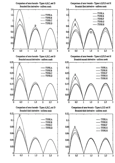
2.4 Results for a uniform mesh

The four graphs in figure 1 below show the pointwise error multipliers K(j, x)

[image:10.595.101.434.164.472.2]

Figure 1: Pointwise error multipliers K(j,x) 0 0 0.35 0.3 0.25 0 0 0.12 0.1

Comparison of error bounds -Types A,B,C, aI¥I D Bounded first derivative - uniform mesh

o.s 1.S

-TYPE A ····-TYPEB ·---·TYPEC --·TYPED·

2 . 2.5

Comparison of error bounds -Types A,B,C, aI¥I D Bounded second derivative - uniform mesh

-TYPEA --·-··TYPE B ---·TYPEC --·TYPED

0.5 1.5 2 2.5

Comparison of error bounds -Types A,B,C, aI¥I D Bounded third derivative - uniform mesh

D

,.,

.

\

-TYPE A I \

···TYPEB

I \

0.08

Ii'\

---·TYPEC --·TYPED 0.06

o.04

I

\

I

\

0.02 I

0

0 0.5 1.5 2 2.5

3

3

3

Comparison of error bounds-Types A,E,F,G and H Bounded first derivative - uniform mesh

1.4.----...----.----..----.----...---, 1.2 0 0 0.35 0.3 0.25 0.2 0.15 0.1 0.05 0 0 0.12 0.1 0.08 0.06 0.04 0.02 0 0 A

o.s l.S

-TYPEA ···TYPEE ---TYPEF --TYPEG ---TYPEH

2 2.5

Comparison of error bounds -Types A,E,F ,0 and H Bounded

secom

derivative - unifonn mesh

-TYPE A -TYPEE ·---TYPEP ·--TYPEO --TYPEH

o.s l.S 2 2.5

Comparison of error bounds -Types A,F,G and H Bounded third derivative - uniform mesh

-TYPEA -TYPEE

A ·---TYPEF _·--TYPEG --TYPEH

o.s l.S 2 2.5

3

3

[image:11.598.69.461.189.744.2]

to be expected because of the semi-local nature of cubic splines.

Comparison of errors -Types A,B,C,D and H Bounded fourth derivative - uniform mesh 0.045.---.---...----,.----.----.---,

0.04

O.D35

0.03

0.025

0.02

O.D15

0.01 0.005

-TYPE A ···TYPEB ... TYPEC -···TYPED - .. - .. -TYPEH

o..._ _ _... __ _.__ __ ...._ _ _,. __ _._ _ __.

0 0.5 1.5 2 2.5 3

We also calculated the norms of s and the derived projectors s1 _{and s}11

for uniform meshes of various sizes, with end intervals included and excluded. The results are shown in tables 3-8 below

The entries in the first of each pair of tables are the usual operator norms,

llLll

= sup

llL/ll[to,tnJ/11/ll[to,tn)

/¢0

while for those in the second the end intervals are excluded in the numerator. Thus,

llLll'

=sup

llL/ll[ti,tn-d/11/ll[to,tn]•

#0

Our interpretation of these results is as follows. For these uniform meshes the various C2 _{methods differ very little when the end intervals are excluded}1

•

Thus once again we see that the end-conditions make a difference only near the end-points. Also, as expected, the operator norms for a particular method hardly change as the the number of intervals in the uniform mesh is increased beyond 8. The error curves for W4 ,00 functions show the C

2 _{methods doing}

better than the strictly local method H in the interior subintervals.

3

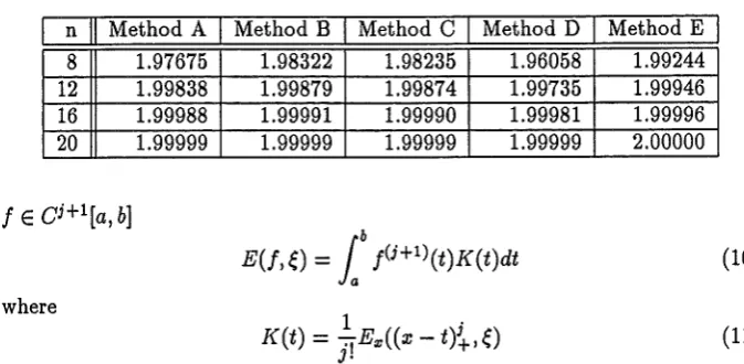
Mathematics underlying the computations

3.1

Calculation of the optimal error bounds.

Fix for the moment the mesh t, the cubic spline interpolant L, and

e

E

[to, tn]

=

[a, b]. Let

E(!, e)

=

t(e) - L(f, e)

Suppose that this error functional anihilates 71'j for some 0 ::; j ::; 3. The application of the Peano kernel theorem (Davis [3], Powell [9]) shows that if

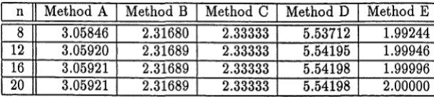
Table 3: Norm of spline operator end intervals included

n II A 1 · B

c

D E F G H 8 1.97098 1.67836 1.71712 2.72960 1.53579 1.53345 1.25000 1.63113 12 1.97164 1.67843 1.71725 2.73294 1.54808 1.54793 1.25000 1.63113

16 1.97164 1.67843 1.71725 2.73296 1.54897 1.54896 1.25000 1.63113 20 1.97164 1.67843 1.71725 2.73296 1.54903 1.54903 1.25000 1.63113

Table 4: Norm of spline operator end intervals excluded

n

II

A B

c

D E F G H

8 1.51768 1.52316 1.52243 1.54745 1.53579 1.53345 1.25000 1.38490 12 1.54666 1.54719 1.54712 1.54903 1.54808 1.54793 1.25000 1.38490 16 1.54887 1.54890 1.54890 1.54904 1.54897 1.54896 1.25000 1.38490 20 1.54902 1.54903 1.54903 1.54904 1.54903 1.54903 1.25000 1.38490

Table 5: Norm of first derived projector end intervals included

n

II

A B

c

D E F G H

8 4.30769 3.33333 3.46392 6.78788 1.73196 2.00000 2.00000 3.33333 12 4.30939 3.33333 3.46410 6.79738 1.73205 2.00000 2.00000 3.33333 16 4.30940 3.33333 3.46410 6.79743 1.73205 2.00000 2.00000 3.33333 20 4.30940 3.33333 3.46410 6.79743 1.73205 2.00000 2.00000 3.33333

Table 6: Norm of first derived projector end intervals excluded

n

II

A B

c

D E F G H

8 1.73120 1.69759 1.69643 2.27352 1.71428 1.71134 1.50000 1.58333 12 1.73205 1.72958 1.72949 2.27669 1.73077 1.73057 1.50000 1.58333 16 1.73205 1.73187 1.73187 2.27671 1.73196 1.73194 1.50000 1.58333 20 1.73205 1.73204 1.73204 2.27671 1.73204 1.73204 1.50000 1.58333

Table 7: Norm of second derived projector end intervals included

n

II

Method A

I

Method B

I

Method C

I

Method D

I

Method E

I

[image:13.597.110.493.193.261.2] [image:13.597.109.494.314.383.2] [image:13.597.130.435.665.733.2]

Table 8: Norm of second derived projector end intervals excluded

n

II

Method A

I

Method B

I

Method C

I

Method D

I

Method E

I

8 1.97675 1.98322 1.98235 1.96058 1.99244 12 1.99838 1.99879 1.99874 1.99735 1.99946 16 1.99988 1.99991 1.99990 1.99981 1.99996 20 1.99999 1.99999 1.99999 1.99999 2.00000

f

E Ci+l[a, b]

where

E(f,e)

=lb

J(i+t)(t)K(t)dt

1 .

K(t)

=

-:rE:ii((x - t)~.e) J.

(10)

(11)

and the notation E:ii ( ( x - t)~, e) means that the functional E( ·, e) is applied to

(x - t)~ considered as a function of x. Because in the case we consider K will have only a finite number of sign changes it follows easily from (10), (11) and smoothing arguments that

sup

IE(f,e)I = llKll1

{/eGi+l [a,bJ:1i/U+1) lloo~l}

or what is equivalent that the least value of C for which the relationship

IE(!,

e)I

~

Cllt(j+l)lloo

holds for all f E Ci+1_[a,

b]

_{is C}

=

llKll1·

_{These conclusions also hold when}

Ci+1_{[a, b] is replaced by W;+t,oo•}

It only remains to discuss how one can calculate K and

llKll1

numerically. Firstly we let { f,i}

?=o

be the cardinal splines corresponding to the interpolant

L. That is .ei is the cubic spline interpolant L(f) when f(tk) = Dik· Th~n for any/,

e

N

L(f,e)

=I:

J(ti)ei(e) i=O

and

n

E(f, e)

=

t(e) -

I:

J(ti).ei(e) i=O

Substituting from (11) it follows that n

j!K(t)

=

(e - t)~

- l:(ti -

t)~.ei(e). (12) i=O

Hence for each 0 ~ j ~ 3, K(t) is a spline of degree j with possible knots at

[image:14.595.105.442.179.344.2]

3.2

Computation of

JJLJJoo

and

JJL'JJoo.

The methods of computing

I ILi ioo

and

llL'lloo

are essentially the same so we will only give the details of the computation of

llL'lloo·

Let

Lf

denote one of the cubic spline interpolants under consideration ap-plied to the function

f

at the nodes t

=to

<

ti

< ...

<

tn.

Then assuming the map L is exact for polynomials of degree j - 1, the derived projector LU) given by

is well defined. We define, as is usual, the operator norm

llL(j)lloo

=

sup

llL(j)(u)ll

gEG(to,tn]:llullco ~ 1

For convenience denote (Lf)(x) by s(x). Assume L is exact for constants. Then considering the matrix system expressing the first derivatives of s at the knots in terms of the data, we see that the linear map from

g

to L'

(g)

may be expressed as the composition of three linear maps

L'

=

EoPoS (13)

where

S : G[t

0 ,

tn] -

IR is the map taking g

=

f'

to the n-vector with ith component

P : IRn - IR2n+l is the map taking the vector a to the 2n

+

1 vector

f3

with ith component

/3

I -

. _ {

ai, I i '

<

n, s

(ti-n),

i ~ n.

and finally,

E :

IR2n+l -

G[to, tn]

is the map taking

f3

to the piecewise quadratic,

s',

with specified endpoint and average values on each subinterval.

Because L' receives only the information about g given to it by the map S

we can rewrite (13) in a form more useful for computation. More precisely, as

g ranges over

{g E

O[to, tn] :

llulloo

~ 1},

S(g) ranges over a set in IRn whose closure is the closed £00 unit ball in IRn. Hence (13) implies

llL'lloo

= sup

ll(E

o

P)(a)lloo

fl={a:llallco~l}

(14)

can be fixed, without loss of generality, the search can be restricted to 2n-l

extreme points. We note that it is known (1] that if L reproduces cubics then llL'lloo cannot be bounded independently oft.

The computation of JJLll00is analogous to that of IJL'IJ00 • In this case

n

is

the £00 _{unit ball in}

IRn+l, extreme points of which correspond to function values [f(to, ... , f(tn)]T to be interpolated. llLIJoo is computed by computing llslloo for

2n of these 2n+l extreme points.

3.3 Computation

of

llL"lloo

When Lis exact for linear polynomials the map

L",

from

i"

to

L"(f"),

is a well defined linear map. It can be written as the composition of three linear maps

L"

=

EoPo S.

Here S maps

f"

to the n - 1 vector of second divided differences b with

1 it;+~

bi= f[ti, ti+1, t;+2]

=

t· t· Ni,2(x)f"(x)dx.

1+2 - I t;

P maps b to the vector of second derivatives u = (s"(ti))?=o and therefore has the form u

=

Db for some ( n

+

1) x ( n - 1) matrix D. Finally E maps the vector of second derivative values u to the piecewise linear interpolant s". 2

Since s" is piecewise linear lls"IJ00 corresponds to a value of s" at one of the

knots. Hence

IJL"lloo

=

m!U sup I

I:

di;f[t;' tj+1, t;+2]I

O:$i:$n {/:/eL"t,,, and llJ"lloo:$1} j

Since values of

!"

in one interval can affect two of the second diffences bi, we cannot simply choose the differences in a bang-bang way as we did in computing IJLJJ and JJL'll· However, fixing i and writing

e;

for di,j

2_{For the}

where

(t·+i -t·) (tJ+1-t;)

w;,

2_=e;(t3 _{/ ) ' w;,1=e;-1(t t )'}

1+2 - j j+l - j-1

and

'· -[ f

0\l-x)f"(t;+(tJ+1-t;)x)dx ] - [ I₀1(l-x)g;(x)dx]

"J - 1 - 1 .

Io xf"(t;

+

_{(tJ+ 1 - t;)x)dx} Io xg;(x)dx

Hence defining A as the closed convex set in

JR.2

A= {[

,\1]

= [

Io~(l-x)g;(x)dx

l:

llulloo

~

1}

,\2 Io xg;(x)dx

the maximum of s"(ti) over functions

f

with

11!"11

~ 1 equals

Here the numbers w;,1c depend only on the mesh t and the matrix D. Hence the problem

(15)

separates into the sum of n two dimensional subproblems

(

n-2 )

max wo 2..\2

+

'°'

max(w; 1..\1

+

W; 2..\2)

+

maxwn-1,1..\1

.\EA ' L..J .\EA '' '' .\EA

j=l

since A is convex the maxima in the subproblems occur at extreme points of A.

Indeed the following lemma shows that the two dimensional subproblems are trivial to solve.

Lemma 1 The set A defined above is the closed convex set with boundary the curves

{ [ a2 _ l ] }

/1 = ..\ = ₂a -

l -

a2 : 0

<

a

<

1

and

/2

= { ,\ = [

.!~

=

t -

a

2

] : 1

>

a

>

o}

together with the points A=

(-!, -!)

and B

= (

!, !) .

Proof:-Omitted.

Having defined A we see that for each non-zero w, wT ,\ is maximized at a unique point on the boundary of A. One can easily calculate that point. For example when w1

>

O, w2

<

0 the maximum corresponds to the unique point in the interior of the lower boundary where w is perpendicular to the tangent. Hence occurs at the point a = - - l £ 1 _ _ ( w ) • Other sign patterns for w are

W1-W2

References

[1] R. K. Beatson, On the convergence of some cubic spline interpolation schemes, SIAM J. Numer. Anal., 23 (1986), pp. 903-912.

[2] C. de Boor A Practical Guide to Splines, Springer-Verlag, New York, 1978. [3] P. J. Davis Interpolation and Approximation, Blaisdell, New York, 1963.

[4]

C. A. Hall On error bounds for cubic spline interpolation, J. Approximation Theory, 1 (1968), 209-218.

[5J C. A . Hall and W. W. Meyer Optimal error bounds for cubic spline inter-polation, J. Approximation Theory, 16 (1976),105-122.

[6] D. Kershaw, Inequalities on the elements of a certain tridiagonal matrix, Math. Comp., 24 (1970), pp.155-158.

[7] D. Kershaw, Two interpolatory cubic splines, J. Inst. Maths Applies 11(1973),329-333.

[8] M. J. Marsden Cubic spline interpolation of continuous functions, J. Ap-proximation Theory, 10 (1974),103-111.

[9] M. J. D. Powell Approximation theory and methods, Cambridge University Press, Cambridge, 1981. · ·