Causal Inference and the Millennium Development Goals (MDGs): Assessing Whether There Was an Acceleration in MDG Development Indicators Following the MDG Declaration

(1)

Causal Inference and the Millennium

Development Goals (MDGs): Assessing

Whether There Was an Acceleration in

MDG Development Indicators Following

the MDG Declaration

Friedman, Howard Steven

Columbia University, School of International and Public Affairs

1 August 2013

Online at

https://mpra.ub.uni-muenchen.de/48793/

(2)

pg 1 | 162

WORKING PAPER

Causal Inference and the Millennium Development Goals (MDGs):

Assessing Whether There Was an Acceleration in MDG Development

Indicators Following the MDG Declaration

The views expressed in this research are those of the author and do not

necessarily reflect the views of the United Nations or UNFPA.

Howard Steven Friedman

School of International and Public Affairs, Columbia University

[email protected]

August 2013

© Howard Steven Friedman 2013

(3)

pg 2 | 162

Abstract

Background: The Millennium Development Goals (MDGs) are a set of eight goals and corresponding indicators that were agreed to following the adoption of the United Nations Millennium Declaration in September 2000 by leaders of 189 countries. The goals state specific objectives for the world to accomplish by measuring progress in indicators during the time period from 1990 (ten years before the declaration) to 2015. While monitoring mechanisms have reported the progress towards achieving these goals, there has been little effort to evaluate whether there was a change in the development outcomes associated with the activities initiated by the MDGs. The dearth of evaluations applied to the MDGs may be associated with the lack of a true counterfactual or the challenges with the data quality. Our analysis focused on the questions of whether there was a statistically significant acceleration or deceleration (mathematically defined as an interrupted slope or intercept) for a particular indicator and, if there was one, whether that changepoint occurred before or after 2001. Accelerations occurring in 2000 or earlier cannot be causally associated with the MDG-related activities (since the acceleration predated the declaration) while accelerations after 2000 may logically be associated with MDG-related activities.

Method: We applied the standard program evaluation methodology of an interrupted time series to the country level yearly measurements of the MDG indicators as well as a set of control indicators that were not included in the set of MDG indicators (and were not likely to have been directly impacted by MDG-related activities). The modeling technique used was a multiple linear mixed model where we identified the optimal year of the changepoint in the outcome by examining years 1992 to 2008 for all datasets.

Analysis was performed separately for IDA-only countries (World Bank 2000 designation) as well as for a broader set of countries consisting of IDA, IBRD and Blend countries. The IDA (International Development Association) focuses on low income countries and the IBRD (International Bank for Reconstruction and Development) focuses on middle income countries. The primary data source for the analysis was the World Bank database where the analysis explicitly assumes that the reported data points are accurate. Reported results contain separate analyses for (1) including heavy influence countries and (2) excluding heavy influence countries; thus resulting in four sets of reported analyses as well as a detailed review of the individual MDG indicator.

Results: The general result was that there was no trend in statistically significant accelerations in the MDG indicators after 2000. Rather the results for all four sets of reported analysis were consistent in that about half of the MDG indicators exhibited no acceleration or deceleration during the time period from 1992 to 2008 and about one-third exhibited accelerations BEFORE 2001. Contrarily, nearly all of the control indicators had no change (neither acceleration nor deceleration) during the time period. It should be emphasized that the control indicators were identified based on data availability and other control indicators may exist that serve as more appropriate controls.

(6)

pg 5 | 162 Discussion: The results may reflect some of the historical nature of the MGDs in that the Millennium Declaration represented a culmination of development agreements and goals that had been established over the preceding years. As such, many of the indicators selected to belong to the MDGs in 2000 had been previously identified in the global development agenda in the 1990s and campaigns to accelerate progress had been initiated before 2000. In fact, when the results of this study have been demonstrated at different United Nations forums, the reaction from seasoned development professionals has consistently been that of affirmation, where the audience generally has indicated that intuitively they would have expected the observed results given their knowledge of how the MDG indicators had been identified. Additionally, the results may be indicative of the impact of long-term broader economic trends where, for example, official development assistance (ODA) comprises only a very minor part of the global economy.

(7)

pg 6 | 162

Introduction

The Millennium Development Goals (MDGs) are a set of eight goals and corresponding indicators that were agreed to following the adoption of the United Nations Millennium Declaration in September 2000 by leaders of 189 countries. The goals state specific objectives for the world to accomplish by measuring progress in indicators during the time period from 1990 (ten years before the declaration) to 2015.

All 193 United Nations member states and at least 23 international organizations have agreed to achieve these goals by the year 2015. The goals (details may be seen in the United Nations website http://www.un.org/millenniumgoals/) are:

Goal 1: Eradicating extreme poverty and hunger, Goal 2: Achieving universal primary education,

Goal 3: Promoting gender equality and empowering women, Goal 4: Reducing child mortality rates,

Goal 5: Improving maternal health,

Goal 6: Combating HIV/AIDS, malaria, and other diseases, Goal 7: Ensuring environmental sustainability, and Goal 8: Developing a global partnership for development.

The goals have been controversial from the onset due to questions regarding the targets that were selected, the indicators chosen, notable omissions such as equality or agriculture, issues with the ability to accurately measure some indicators such as maternal mortality, malaria and tuberculosis and concerns about possible unintended consequences (such as a focus on primary enrollment potentially diminishing educational quality).

From a historical perspective, it is important to note that the declaration of the MDGs and the Millennium Summit did not represent the start of global movements towards issues of poverty, health, education and other key subjects. Rather, the Millennium Summit and corresponding declaration of the MDGs may be viewed as the culmination of many agreements and processes that had been occurring in the previous decade. The summit itself represented a means for the United Nations to solidify its role and position in the 21st century (United Nations 2000, We the Peoples) and reinvigorate the global community to refocus on development following a number of years of reduced Official Development Assistance (ODA) in the late 1990s. Many of the targets and indicators used in the MDGs were derived

from indicators and targets established through various international conferences in the 1990’s.

Global events and declarations that preceded the Millennium Summit that contributed to the identification of goals, targets and indicators include (but are not limited to):

1987:

 WHO launches the Global Program on AIDS.

 General Assembly resolves to mobilize the entire UN system in the worldwide struggle against AIDS and designates the WHO to lead the effort.

1990

(8)

pg 7 | 162

 World Declaration on Education for All adopted by the World Conference on Education For All, launching a global movement to provide basic education for all children, youth and adults.

1993:

 Declaration on the Elimination of Violence against Women (1993) was adopted, providing a framework for analysis and action at the national and international levels.

 International Congress and World Plan of Action on Education for Human Rights and Democracy (Montreal, Canada).

1994:

 International Conference on Population and Development (ICPD) Conference and Program of Action. Within the Program of Action, a large number of key areas of focus were identified that later became components of the Millennium Development Goals.

1995:

 The U.S. Food and Drug Administration (FDA) approved the first protease inhibitor initiating the era of highly active antiretroviral therapy (HAART).

 DOTS (Directly Observed Treatment, Short-course) Strategy launched.

 Declaration and Integrated Framework of Action on Education for Peace, Human Rights and Democracy, ICE (Geneva, Switzerland).

1996:

 UNAIDS begins operations bringing renewed focus and attention to HIV/AIDS;

 International AIDS Vaccine Initiative Exit Disclaimer (IAVI) forms to speed the search for an effective HIV vaccine.

 World Bank releases report on poverty titled “Poverty Reduction and the World Bank: Progress

and Challenges in the 1990s”

 Heavily Indebted Poor Countries (HIPC) Program initiation by World Bank and IMF though initial uptake is low

1997:

 Highly active antiretroviral therapy (HAART) becomes the new standard of HIV care.

 Multilateral Initiative on Malaria founded to strengthen Africa’s ability to spearhead new malaria approaches

1998:

 Roll Back Malaria Partnership (RBM) launched by WHO, UNICEF, UNDP and World Bank with goal of halving malaria incidence and mortality by 2010

1999:

 World Bank publishes World Development Indicators 1999, warning that the new millennium could reverse the development gains recently made, and that new strategies are needed for the future.

 Operational Review and Appraisal of the Implementation of the International Conference on Population and Development (ICPD) Programme of Action raises concerns about overall progress.

2000:

 Heavily Indebted Poor Countries (HIPC) Program accelerated with 22 countries (18 in Africa) benefitting by end of year.

(9)

pg 8 | 162

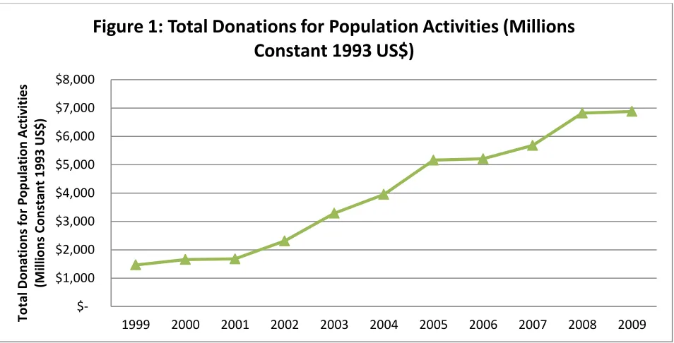
The Millennium Development goals succeeded at raising the global awareness of investing in development. As will be discussed later, there was a demonstrable increase in the amount of donor funding for development following the MDG Declaration. For example, as reported in the Financial Resource Flows for Population Activities (UNFPA, 2009), the donor funding for population activities in 2009 was nearly 5 times more than the amount provided in 1999.

Source: Financial Resource Flows for Population Activities (UNFPA, 2009)

Associated with the Millennium Development Goals was the enhanced investment in monitoring systems including support for census, vital registrations, surveys and analysis, all with the goal of better assessing progress towards achievement of the goals. Information regarding the progress towards achieving the MDGs is readily available on the internet at various UN-sponsored websites (see http://www.un.org/millenniumgoals/ and http://data.worldbank.org for example). These sources and

other publications regularly report which indicators are “on track” or “off track”, a reflection of whether

or not those indicators are expected to achieve their targets by 2015. This monitoring of progress is important in assessing how countries are performing with respect to the MDGs but it is distinct from evaluation, the process of determining if the MDGs (declaration and resulting activities) causally impacted the outcomes of interest, the targets and indicators of development included in the MDGs.

To our knowledge, our study will be one of the first studies that specifically compare the rate of progress

on the MDG indicators before and after the initiation of the MDG’s in 2000, and the only one that

conducts this analysis systematically for the entire set of MDG indicators using a rigorous quasi-experimental method. Rajaratnam et al (2010) assessed levels and trends in child mortality for 187 countries from 1970 to 2010 and found evidence of acceleration in rates of decline in child mortality –

$1,000 $2,000 $3,000 $4,000 $5,000 $6,000 $7,000 $8,000

1999 2000 2001 2002 2003 2004 2005 2006 2007 2008 2009

[image:9.612.75.552.209.452.2]

To tal Do n ation s for Po p u lation Ac tiv ities (M il li o n s Co n stan t 1993 US $)

(10)

pg 9 | 162

31% of countries had rates of decline above the MDG 4 target rate of 4.4% per year from 1990-2000, and the figure increased to 34% from 2000-2010. However, it was not stated if the increase was statistically significant. Another study by You et al (2009) compared the rate of decline in under-five mortality rates in the 1990s with that in 2000-2008 and concluded that the rate has increased – although statistical significance was not examined. They also attributed the acceleration in progress to MDG activities such as improvements in coverage of bed nets and better delivery of vaccinations, although a formal link was not established. Moreover, those studies did not employ the methodologies of analyzing time series data to identify the time at which the program began accelerating but rather simply tried to argue about the result in aggregate. Beyond these studies, we did not find other studies that attempted to draw a causal link between the initiation of the MDGs and any acceleration or improvements in the MDG indicators.

Other studies surrounding the MDG indicators focus on analyzing and projecting trends in order to identify countries or regions that are on track to achieving the MDG targets in 2015 (Lozano et al., 2011; Sahn, David and Stifel, 2003; Leo, Benjamin and Ross, 2011; Economic Commission for Europe, 2006; Ritu and Rokx, 2004; Ram, Mohanty and Ram, 2009). It was generally found that regions such as Latin America/Caribbean, Asia and Central Europe are doing well, while regions such as Africa are below the achievement trajectory.

Many other studies focus on qualitative analysis of the MDG framework and make recommendations on how it could be altered to support the achievement of the MDGs, for example: improving data quality (Attaran, 2005; Murray, 2007); instituting a new MDG review process (Sumner, Andrew and Lawo, 2010); addressing issues on institutional quality and fiscal challenges (UNDP, 2010); improving country ownership (HuRiLINK, 2012); improving microfinance (Littlefield, Murduch and Hashemi, 2003); and redistributing or increasing aid (Gwatkin, 2002; Herfkens, Eveline and Bains; Radelet, 2004; World Bank, 2010).

This is an opportune time to examine the question of whether or not the MDGs stimulated an acceleration in key indicators of global development. 2013 marks a critical point in development work – growth in the global economy is slowing, donor funding is being challenged and the lack of progress in development is causing concern. Amid these challenges, UN Task Teams are exploring the establishment of new development goals that are inclusive of other aspects of development neglected by the Millennium Development Goals (MDG), activities grouped together as the “Post-2015 Planning”. These new targets will stimulate interest and investment in specific areas related to development but overhead floats the critical question of whether these MDG-related development activities have had a significant impact on development progress since 2000?

(11)

pg 10 | 162

To draw a causal inference regarding the relationship between the MDG-related activity and development progress, one can think of the conditions identified by John Stuart Mill for causal inference: (1) that the cause precedes the effect, (2) that the cause is related to the effect and (3) that there are no other plausible explanations other than the cause. In determining whether there is a causal relationship between the MDG Declaration and resulting activities, the analysis is complicated by the facts that virtually the entire world was involved in the declaration (so there is no true control population that was not impacted by the MDG Declaration and resulting activities) and that the goals were declared 40% of the way into the time period stated for the target (1990 to 2015).

In order to test the hypothesis of whether or not there was an acceleration in development indicators associated with the MDGs, we invoked the quasi-experimental program evaluation method of interrupted time series and applied this to the MDG identified indicators. The math technique used for this analysis, described in more detail later, is a multiple linear mixed model. This mathematical functional form is appropriate for data of this structure in that it accounts for the correlations among repeated observations from the same country while the assumptions of simpler approaches such as multiple linear regression models are violated under these circumstances.

The interrupted time series method allows us to identify if there was an acceleration (interrupted slope) for the time series measurements. For datasets where there was an acceleration, the year of the interruption was compared with the timing of the MDG activity. As a secondary measure, we also explored if there was a step change in the development indicators (interrupted intercept) though this is not generally considered likely given the fact that global development programs scale up over time and

don’t usually have a ramp-up of less than one year. Logically, if there is no measurable acceleration or

step-up (no interrupted slope or interrupted intercept) between 1990 and 2010 in the MDG indicators, then we cannot say that the development activities during that time period accelerated development progress for those specific MDG indicators. If there was an acceleration in development outcomes that was associated with MDG-related activity, then, in order for it to be causally-related to the MDG Declaration, the acceleration had to start in 2001 or later since the declaration was in September 2000. This is a consequence of assumption (1) above for causal inference. Accelerations that occur before the MDG Declaration (before 2000) cannot be causally linked to the MDGs (a breakdown in assumption (1) above) but may be causally linked to the activities that preceded the MDGs.

Additionally, a set of control time series datasets were selected by identifying data series that were important to development but not included in the MDGs and would not likely have been directly impacted by the MDGs. The control set of indicators presents an additional test of the causal relationship of the MDGs to development. Logically, it is not absolutely necessary to have control indicators since in an interrupted time series analysis, the pre-declaration time period acts as the control for the post-index time period for the MDG indicators. That is to say, one could describe the MDGs a pre-post design with multiple pre and post measurements and no control.

(12)

pg 11 | 162

the MDGs then it would suggest a breakdown in assumption (3) above for causal inference. That is, if both the MDG-related indicators and indicators that are not clearly related to the MDGs experience the same patterns of acceleration or deceleration then one should look for other plausible explanations for the acceleration beyond the MDG-related activity.

Data Sources

DATA SOURCES

While the primary data source was the World Bank Database (http://data.worldbank.org/), data was also extracted from the UNICEF and the World Health Organization (WHO) databases to ensure standardization across all countries. Our analysis focuses on developing countries, which we define as countries classified into the World Bank’s IDA, IBRD and Blend1 lending categories in 20002. Countries in these categories have been identified by the World Bank to be in need of developmental aid, with low income IDA countries displaying the greatest need. Data was analyzed for two groups of developing countries, where group 1 consisted of the IDA, IBRD and Blend countries (low and middle income) while group 2 consisted of only the IDA countries (low income only countries).

Data was extracted between September 2012 and November 2012 and reflects the latest data available at the time of data extraction.

SELECTION CRITERIA

We defined the following objective criteria for selection of indicators:

1. Data availability: annual data should be publicly available for the time period 1990-2010 so that the analysis could be readily replicated by other researchers.

2. Data volume: annual data should be available for at least 50 countries in the IDA, IBRD and Blend categories for at least 10 consecutive time points from 1990-2010 where the time period begins before 1998.

MDGINDICATORS

44 MDG indicators were listed in the World Bank database. Of these, 19 were found to match the criteria above. Appendix A contains descriptions of the 25 indicators that did not match our selection criteria. We replaced World Bank statistics for the under-five mortality rate and the infant mortality rate with the most recent 2012 data from the UNICEF Child Mortality Estimates (CME) database.3

1

IDA countries are those that had a per capita income in 2011 of less than $1,195 and lack the financial ability to borrow from IBRD. IDA loans are deeply concessional—interest-free loans and grants for programs aimed at boosting economic growth and improving living conditions. IBRD loans are nonconcessional. Blend countries are eligible for IDA loans because of their low per capita incomes but are also eligible for IBRD loans because they are financially creditworthy. For more information see: http://data.worldbank.org/about/country-classifications 2

Lending categories in 2000 were selected instead of those in more recent years to avoid selection bias – since countries that did well economically and developmentally were more likely to graduate from the IDA, IBRD and Blend lending categories, thus skewing the sample of IDA, IBRD and Blend countries in more recent years towards countries that showed slower progress in development.

3

(13)

pg 12 | 162

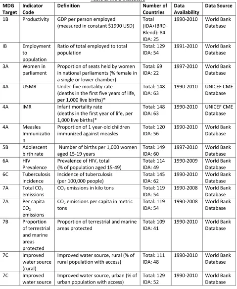
[image:13.612.68.547.140.723.2]

Table 1 describes the complete list of MDG indicators in our study:

Table 1: MDG Indicators MDG

Target

Indicator Code

Definition Number of

Countries

Data Availability

Data Source

1B Productivity GDP per person employed

(measured in constant $1990 USD)

Total (IDA+IBRD+ Blend): 84 IDA: 25

1990-2010 World Bank Database

IB Employment to

population

Ratio of total employed to total population

Total: 129 IDA: 54

3A Women in parliament

Proportion of seats held by women in national parliaments (% female in a single or lower chamber)

Total: 69 IDA: 22

4A U5MR Under-five mortality rate

(deaths in the first five years of life, per 1,000 live births)*

Total: 148 IDA: 63

1990-2010 UNICEF CME Database

4A IMR Infant mortality rate

(deaths in the first year of life, per 1,000 live births)*

Total: 148 IDA: 63

1990-2010 UNICEF CME Database

4A Measles Immunizatio n

Proportion of 1 year-old children immunized against measles

Total: 120 IDA: 56

5B Adolescent birth rate

Number of births per 1,000 women aged 15-19 years

Total: 149 IDA: 60

1997-2010 World Bank Database 6A HIV

Prevalence

Prevalence of HIV, total (% of population aged 15-49)

Total: 114 IDA: 49

1990-2009 World Bank Database 6C Tuberculosis

incidence

Incidence of tuberculosis (per 100,000 people)

Total: 145 IDA: 62

1990-2010 World Bank Database 7A Total CO2

emissions

CO2 emissions in kilo tons Total: 119 IDA: 54

1990-2008 World Bank Database 7A Per capita

CO2 emissions

CO2 emissions per capita in metric tons

Total: 119 IDA: 54

7B Proportion of terrestrial and marine areas protected

Proportion of terrestrial and marine areas protected

Total: 109 IDA: 41

7C Improved water source (rural)

Improved water source, rural (% of rural population with access)

Total: 111 IDA: 48

7C Improved water source

Improved water source, urban (% of urban population with access)

Total: 129 IDA: 52

(14)

pg 13 | 162

(urban) 7C Improved

sanitation (rural)

Improved sanitation facilities, rural (% of rural population with access)

Total: 105 IDA: 44

7C Improved sanitation (urban)

Improved sanitation facilities, urban (% of urban population with access)

Total: 115 IDA: 45

8A Total ODA Net official development assistance received (measured in current US$)

Total: 115 IDA: 57

1990-2010 World Bank Database 8A ODA (%GNI) Net official development assistance

received (measured as percentage of gross national income)

Total: 101 IDA: 47

8D Debt service Total debt service as % of exports of goods and services and net income

Total: 67 IDA: 24

(15)

pg 14 | 162

CONTROL INDICATORS

The control indicators used in this analysis were identified based on their ease of availability and hence the control datasets are not ideal controls. Better controls would be indicators that (1) were considered for the MDGs but eventually not selected and (2) are not closely related to the selected MDG indicators in terms of activities or outcomes.

For this study, we leveraged the World Bank Database that, as of 4Q 2012 contained 1260 indicators. From the list of 1260 indicators, we identified 377 indicators where annual data from 1990-2010 was available. Of these, 343 were discarded as they were either: (1) MDG indicators; (2) closely related to the MDG indicators (e.g. fertility rate was discarded as the MDG indicator of adolescent birth rate is a subset of fertility rate); (3) related specifically to World Bank financing and not of interest to our study (e.g. currency composition of granted debt); or (4) completely unrelated to development (e.g. land area).

The remaining 24 indicators fall into the broad categories of life expectancy, agricultural development, financial investment and military expenses. We left out the category of life expectancy from the set of controls since life expectancy is strongly determined by infant mortality rate, U5 mortality rate, HIV rate and other MDG indicators. We selected 7 indicators from the remaining categories. Appendix B contains a description of indicators within this group that were not selected for our study.

Aside from indicators on agricultural development, investment and military expenses, we would have liked to have important health-specific development indicators that were not included in the MDGs, for example cardiovascular mortality rates, but data was generally not available. These indicators of non-communicable diseases are receiving increasing attention by developing countries and may likely play a prominent role in the post-2015 MDG discussion. Additionally, other control indicators that were desirable, but not available, included the incidence of child marriage or child labor measures.

We did manage to identify WHO data on lung cancer mortality produced by the International Agency for Research on Cancer for a small sample of 23 countries from 1990-2010. Lung cancer was specifically chosen as it is the leading cancer in many countries. Although the sample size was smaller than our selection criterion, we decided to include it as a health-specific control indicator for comparison with the health-related MDG indicators.

Of the control indicators selected, crop production and food production can easily be argued to be important for development but not included in the MDGs. Armed forces and military expenditures can be argued to be related to whether the planet is becoming more or less violent/militarized where one can easily conceive that a more peaceful planet is an important goal.

(16)

[image:16.612.65.557.115.461.2]

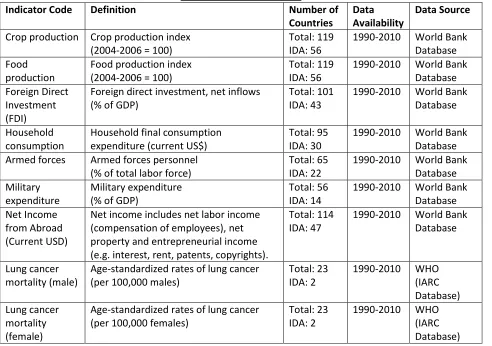
pg 15 | 162 Table 2: Control Indicators

Indicator Code Definition Number of

Countries

Data Availability

Data Source

Crop production Crop production index (2004-2006 = 100)

Total: 119 IDA: 56

1990-2010 World Bank Database Food

production

Food production index (2004-2006 = 100)

Total: 119 IDA: 56

1990-2010 World Bank Database Foreign Direct

Investment (FDI)

Foreign direct investment, net inflows (% of GDP)

Total: 101 IDA: 43

Household consumption

Household final consumption expenditure (current US$)

Total: 95 IDA: 30

1990-2010 World Bank Database Armed forces Armed forces personnel

(% of total labor force)

Total: 65 IDA: 22

1990-2010 World Bank Database Military

expenditure

Military expenditure (% of GDP)

Total: 56 IDA: 14

1990-2010 World Bank Database Net Income

from Abroad (Current USD)

Net income includes net labor income (compensation of employees), net property and entrepreneurial income (e.g. interest, rent, patents, copyrights).

Total: 114 IDA: 47

Lung cancer mortality (male)

Age-standardized rates of lung cancer (per 100,000 males)

Total: 23 IDA: 2

1990-2010 WHO (IARC Database) Lung cancer

mortality (female)

Age-standardized rates of lung cancer (per 100,000 females)

Total: 23 IDA: 2

(17)

pg 16 | 162

Methodology and Modeling

OBJECTIVES

We aim to explore three questions: (1) was there a statistically significant interruption in the time series; (2) if there was an interruption in the time series, was there an acceleration or deceleration of progress towards the MDGs; and (3) did the interruption occur before or after the MDG Declaration in September 2000? These questions allow us to identify if the initiation of the MDGs was associated with any acceleration in progress on the MDG development indicators.

We then go a step further to try to draw a causal link between the initiation of the MDGs and any acceleration in progress on the MDG indicators. If the acceleration in progress on the MDG indicators was not specifically associated with the activities and programs surrounding the initiation of the MDGs, but was reflecting an overall improvement in development due to other factors, we would expect our control indicators to show the same pattern of accelerated progress. Hence, we ran the same models on our selected control indicators to identify if the same pattern of acceleration (or deceleration) occurred.

THE MODEL

We took the systematic approach of modeling all data as having a trend line and a single interrupted year where that interruption could be an interrupted slope and interrupted intercept. Proposed

“interrupted years” encompassed all years in the dataset excluding the end points (i.e. a dataset with

values from 1990-2010 was tested for 17 proposed interruptions in 1992, 1993 and so on until 2008).

As shown below, we used a linear mixed model with an interrupted intercept and an interrupted slope. We also explored other models with only the interrupted intercept or only the interrupted slope, but found the model below to be the optimal model as it was general enough to be systematically applied to all datasets used.

( )

where:

 is the dependent variable, which is either an MDG or control indicator. We used logged values to minimize the effect of heavy influence countries and bring the raw data closer to a normal distribution. Since we are using logged values, a unit increase in any of the independent variables, say a 1 unit increase in , leads to a % increase in y.

 is a constant term representing the intercept.

 are fixed effect coefficients.

 is the time variable taking on the values [-10,10], as the time period [1990,2010] was standardized to [-10,10]. The coefficient is the growth rate, representing a 100 change in every year.

 is a binary variable where

{

A statistically significant coefficient represents a step change in the time series (i.e. a change in the intercept or interrupted intercept) starting at the interrupted year.

 is a variable where

(18)

pg 17 | 162

A statistically significant coefficient represents a slope change in the time series (i.e. a change in the slope or interrupted slope) starting at the interrupted year. The correlation matrix was assumed to be unstructured.

Linear mixed models were constructed for each indicator for each possible interrupted year. The optimal interrupted year corresponded to the interrupted year that gave the maximum goodness of fit for the model (i.e. the minimum Bayes Information Criterion, BIC). The model for the optimal year was used to identify if there was a statistically significant interruption in the trend. Later, it was also used to identify heavy influence countries for robustness checks.

We are primarily interested in looking for a statistically significant coefficient as it represents a slope change in the time series starting at the interrupted year. This represents the most plausible way in which the MDGs could have impacted the indicators. The direction of and was examined to determine if it suggested an acceleration or a deceleration in the trend. For a few indicators, there appeared to have been a significant interrupted intercept rather than an interrupted slope – indicating that there was a step shift in the optimal year rather than a change in the trend.

 are country-specific random effect coefficients. We assume that coefficients for the intercept, trend, interrupted year and interrupted slope may vary by country. Further, we place no constraints on the covariance matrix for these random effects, such that:

[ ] [(

)]

Lastly, is an individual-level error term where ( ).

ILLUSTRATION OF HOW THE MODEL WORKS

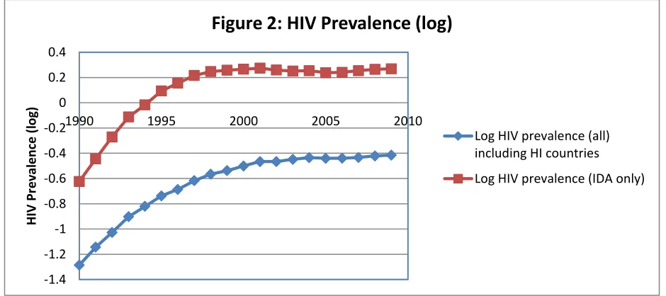
We demonstrate the specific steps in our analysis using HIV prevalence as an example. We then display other examples where an interrupted time series was identified by the model, and where there was no interruption in the time series. A full description of the analysis appears for each MDG in Appendix C.

(19)

pg 18 | 162

The steps in our analysis are:

(1) Transform the y-variable (in this case HIV prevalence) to log HIV prevalence and examine the distribution.

(2) Develop time series projections using 1990-1999 as baseline years and then explore visually if there appears to have been an interruption in the time series, and, if so, whether the visual inspection suggests when the interruption occurred. The HIV curve was compared with time series projections of the outcome variable where the time period 1990 to 1999 was used as an input and the time series projection was produced for the period 2000 to 2010. In addition to the time series, a linear regression model was developed using time as the x-variable and the indicator variable as the y for the time period 1990 to 1999 and then extrapolated to cover the period 2000 to 2010. The regression model was produced as a back-up in case other time series forecasting methods did not converge though it is known that the input time series data violates basic assumptions of linear regression. Visual inspection was then performed on three curves, the actual time series of the indicator, the time series projection and the regression projection. For the example above, the HIV prevalence data indicates that there was an interrupted slope

starting in the late 1990’s for both the IDA-only countries and the IDA, IBRD and Blend countries.

That is to say, the rate of increase in the log HIV prevalence changed starting in the late 1990’s

based on visual inspection and comparison with time series projections (see Figure 11)

(3) Using the full dataset (1990-2010), construct a linear mixed model for the target variable for each potential interrupted year ranging from 1992 to 2008.

(4) Record the Bayes Information Criterion (BIC), interrupted intercept coefficient, interrupted slope coefficient, and corresponding p-values for each potential interrupted year from 1992 to 2008.

(5) Select the interrupted year corresponding to the minimum BIC. Since each of these interrupted year models has the same number of degrees of freedom, the model with the minimum BIC is representing the model that explains the greatest amount of variability in the dataset.

The proposed interrupted year that produced the lowest value for the BIC was identified as the year in which an interruption in the time series trend occurred.

The BIC is calculated as follows:

-1.4 -1.2 -1 -0.8 -0.6 -0.4 -0.2 0 0.2 0.4

1990 1995 2000 2005 2010

[image:19.612.71.541.104.313.2]

H IV Pr e v al e n ce ( lo g )

Figure 2: HIV Prevalence (log)

Log HIV prevalence (all) including HI countries

(20)

pg 19 | 162

( | ) ( )

where:

x is the observed data

n is the number of data points in x, (or the sample size)

k is the number of free parameters to be estimated.

p(x|k) is the likelihood of the parameters given the dataset

L is the maximized value of the likelihood function for the estimated model.

Below is the plot of BIC as a function of year for the log HIV prevalence model. One can easily see that the minimum BIC occurred in 1997 for the IDA, IBRD and Blend dataset displayed below. This year corresponds well to the year identified via visual inspection (Figure 2) and in comparison to the time series projections (Figure 11).

(6) Record the coefficients on the interrupted slope and intercept for the model with the optimal interrupted year – the year that gives the best goodness of fit (i.e. minimum BIC). In this example, the optimal model had an interrupted year in 1997, and a statistically significant interrupted slope (p<0.0001) that was negative. This negative interrupted slope indicates that the annual increase in HIV prevalence started slowing down around 1997.

(7) Predict log HIV prevalence using the model with the selected year (in this case 1997) and compare it to the actuals. We can see below that the predicted curve is very close to the observed curve.

-2000 -1500 -1000 -500 0 500 1000

1990 1995 2000 2005 2010

[image:20.612.94.531.305.569.2]

BIC

Figure 3: Bayes Information Criterion (BIC curves (HIV))

BIC (all), including HI countries

(21)

pg 20 | 162

(8) Identify the heavy influence countries by selecting countries that had a Restricted Likelihood Distance > 5 or a Cook’s distance >0.3. In the case of HIV prevalence, only one country was identified as a heavy influence country, the Russian Federation.

(9) Remove the heavy influence countries and repeat steps (2) through (7) noting any major

changes in the model interpretations based on including or dropping heavy influence countries. The heavy influence countries are important as they point to countries whose patterns were different than the global trends. The heavy influence countries may represent positive or negative patterns and, as such, can point to potential future research.

(10)A fixed effect polynomial time function was added to the interrupted time series model to see if the results were robust to the more complicated model structure. It is important to note that the interpretation of the interrupted slope/intercept in a fixed effect polynomial time function is different from that of a linear time function and so conclusions drawn on this model should be taken with care. From a computational point of view, when a fixed effect polynomial time function is added to the model, this means that the interrupted slope/intercept must be incremental to the polynomial curvature. Specifically, a time series that is well fit by a second order time polynomial will likely be identified as having (a) a statistically significant interrupted slope/intercept when there is only a first order fixed effect time polynomial but (b) not having a statistically significant interrupted slope/intercept when a second order fixed effect time polynomial is added since the second order polynomial captures the shift in the time series that was represented by the interrupted slope/intercept in the first order fixed effect model.

This same methodology of analysis was replicated for all indicators.

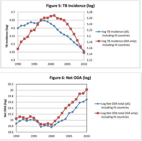
Aside from HIV prevalence, a clear interruption was seen for tuberculosis incidence (interruption in 1999/2000); total ODA (interruption in 1999) and GDP per person employed (interruption in 1996) as shown below.

-1.4 -1.2 -1 -0.8 -0.6 -0.4 -0.2 0

1990 1995 2000 2005 2010

H

IV

Pr

e

v

al

an

ce

(

lo

g

[image:21.612.102.529.105.323.2]

)

Figure 4: Actual versus Predictive HIV Prevalence (log)

Log HIV prevalence (all) including HI countries

Predicted Log HIV

(22)

pg 21 | 162 5.12 5.14 5.16 5.18 5.2 5.22 5.24 5.26 5.28 4.4 4.45 4.5 4.55 4.6 4.65 4.7

1990 1995 2000 2005 2010

[image:22.612.79.536.102.554.2]

TB In ci d e n ce (l o g )

Figure 5: TB Incidence (log)

log TB incidence (all); including HI countries

log TB incidence (IDA only); including HI countries

18.6 18.8 19 19.2 19.4 19.6 19.8 20 20.2

1990 1995 2000 2005 2010

N e t OD A (l o g )

Figure 6: Net ODA (log)

Log Net ODA total (all); including HI countries

(23)

pg 22 | 162

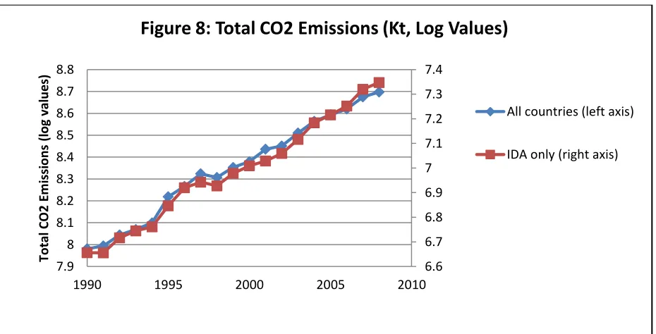
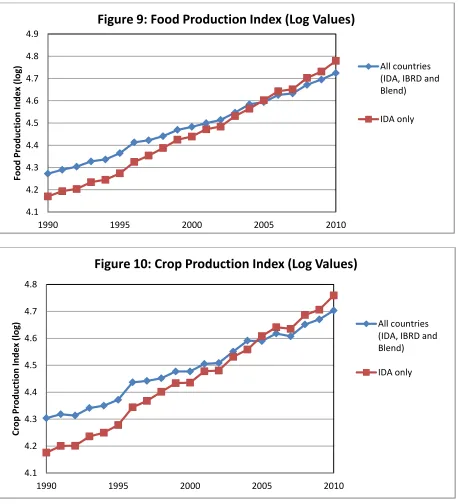
Our model did not identify an interruption in the total CO2 emissions nor in most of the control indicators such as food production. Visually, these graphs present as near-straight lines with no changes in slope as shown in Figures 5-7.

7.7 7.75 7.8 7.85 7.9 7.95 8 8.05 8.1 8.75 8.8 8.85 8.9 8.95 9 9.05 9.1 9.15 9.2 9.25 9.3

1990 1995 2000 2005 2010

[image:23.612.73.539.102.322.2]

GDP p e r p e rson e m p lo y e d (l o g )

Figure 7: GDP per person employed (log)

Log gdp per employee (all) primary axis

Log gdp per employee (IDA only) secondary axis

6.6 6.7 6.8 6.9 7 7.1 7.2 7.3 7.4 7.9 8 8.1 8.2 8.3 8.4 8.5 8.6 8.7 8.8

1990 1995 2000 2005 2010

To tal CO2 E m issi o n s (l o g v al u e s)

Figure 8: Total CO2 Emissions (Kt, Log Values)

All countries (left axis)

[image:23.612.75.540.385.622.2]

(24)

pg 23 | 162

ROBUSTNESS CHECKS

We ran 5 different robustness checks for our model to ensure the reliability of our results:

(a)Removing heavy influence countries

Heavy influence countries in each dataset were identified using Cook’s distance (>0.3) and Restricted Likelihood Distance (>5). The heavy influence countries were dropped and the regressions were

re-4.1 4.2 4.3 4.4 4.5 4.6 4.7 4.8 4.9

1990 1995 2000 2005 2010

[image:24.612.79.537.101.605.2]

Fo o d Pr o d u ction In d e x (log)

Figure 9: Food Production Index (Log Values)

All countries (IDA, IBRD and Blend) IDA only 4.1 4.2 4.3 4.4 4.5 4.6 4.7 4.8

1990 1995 2000 2005 2010

Cr o p Pr o d u ction In d e x (l o g )

Figure 10: Crop Production Index (Log Values)

All countries (IDA, IBRD and Blend)

(25)

pg 24 | 162

estimated. It was found that, in most cases, removing heavy influence countries did not generally alter the conclusions of the analysis.

(b)Examining quality of fit by analyzing residuals

The quality of fit of the model to the data was assessed by examining the pattern and magnitude of the residuals. The Kolmogorov-Smirnov test revealed that the residuals did not fit a normal distribution. However, the magnitude of the residuals was comparatively small. We measured the magnitude of residuals using the absolute percent deviation from the actual, or

| | . This absolute percent deviation was less than 1% for most of the datasets. For 5 datasets, the residuals were slightly larger at about 2-7%, with residuals for a few years going above that (but still below 25% of the magnitude of the actual log values). These data sets with larger absolute percent deviations tended to have denominators close to zero thus inflating the measured absolute percent deviation. In general, the quality of fit was satisfactory for most indicators.

(c)Visual inspection

We also used visual inspection to examine whether the year where an interruption in the time series occurred (as identified by the statistical analysis) agreed with visual inspection of the graphs of the raw data. The results from the interrupted time series analysis generally concurred with the results from visual inspections.

(d)Least squares and time series projections

In order to supplement the visual inspection, we made use of data from all countries from 1990-1999 to project outcomes post-2000. Both least squares and time series projections were used. The actual data was compared with the projections to see if an interruption in the time series occurred after 2000.

(26)

pg 25 | 162

The projections indicated a significant interruption in the time series around 1999 for HIV prevalence and no interruption in the time series for total CO2 emissions. These visual inspection observations are in line with our modeling results (statistically significant interruption in 1997 for HIV prevalence and no statistically significant interruption for CO2 emissions respectively). In general, the statistically derived results agreed with visual inspection.

(e)Including fixed effect polynomial variable -1.4 -1.2 -1.0 -0.8 -0.6 -0.4 -0.2 0.0 0.2 0.4 0.6

1990 1995 2000 2005 2010

[image:26.612.82.528.100.614.2]

H IV Pr e v al e n ce ( lo g )

Figure 11: HIV Prevalence (Log Actual Values vs.

Projections using 1990-99 data)

Actual HIV Prevalence (Log Values) Least Squares projection Time series projection 7.9 8.0 8.1 8.2 8.3 8.4 8.5 8.6 8.7 8.8 8.9

1990 1995 2000 2005 2010

To tal CO2 E m issi o n s (K t, Log val u e s)

Figure 12: Total CO2 Emissions (Log Actual Values vs.

Projections using 1990-99 data)

(27)

pg 26 | 162

As a model with two trend lines may be criticized for not being able to fit the data well, we added a fixed effect polynomial term (a squared time variable) to our regressions to see if it impacted our results. It should be noted that using a polynomial term in an interrupted time series shifts the interpretation of the interrupted slope and intercept coefficients – we are no longer testing if there was a shift from a linear trend but rather testing if there was a shift from a polynomial trend. As a result of this shift in interpretation of the interrupted slope and intercept coefficients, this analysis is not a focus of the study but the results are nonetheless reported.

Our new model is as follows:

( )

(28)

pg 27 | 162

Results and Analysis

Before presenting a more detailed review of the results, we will first present summary tables and graphs representing the overall trends. Detailed analyses of each MDG indicator are provided in Appendix C.

As seen in Table 3, about half of the MDG indicators and the vast majority of the non-MDG indicators had no acceleration or deceleration during the observation period 1990 to 2010. The MDG indicators that had an acceleration nearly universally experienced that acceleration in 2000 or earlier, meaning that the acceleration could not have causally been linked to the MDG Declaration. The primary exception to this observation was the MDG indicator related to total debt service where the shift occurred around 2001/2002.

There were some MDG indicators that experienced decelerations, rather than accelerations. Some of these decelerating MDGs are indicators that have a maximum of 100%. While this could plausibly be due to a ceiling effect, the actual values were generally noticeably below 100% so the ceiling effect concerns are not likely to be a primary explanation. Examples of indicators that had some form of a deceleration during the time period include proportion of terrestrial and marine areas protected,

(29)

[image:29.612.72.563.123.443.2]

pg 28 | 162 Table 3: Summary results of Interrupted Time Series Analysis

MDG Indicators (19 indicators)

IDA, IBRD and Blend Countries IDA Only

All countries

Dropping HI countries

No Acceleration or Deceleration 10 6 12 10

Acceleration 2000 or before 6 6 6 4

Acceleration 2001 or after 1 2 1 3

Deceleration 2000 or before 1 2 0 2

Deceleration 2001 or after 1 3 0 0

Non-MDG Indicators (9 indicators)

IDA, IBRD and Blend Countries IDA Only

No Acceleration or Deceleration 6 6 5 5

Acceleration 2000 or before 0 0 0 0

Acceleration 2001 or after 1 1 1 1

Deceleration 2000 or before 1 1 1 1

Deceleration 2001 or after 0 0 0 0

Modeling limitations* 1 1 2 2

*Modeling limitations means either the model did not converge or that there were not enough countries to run the model.

For the more detailed summary presentation, we present the following items in our results table for two categories – all countries (IDA, IBRD and Blend); and IDA countries only:

(a)The interrupted year – as identified by the optimal proposed interrupted year, that is, the proposed interrupted year that corresponds to the lowest BIC for all regressions on a dataset.

(b)Statistical significance (of and ) the coefficients on the interrupted slope and interrupted intercept variables. We are primarily interested in identifying if the model had a statistically significant which would indicate that there was a statistically significant interrupted slope in the time series in the identified year but we also identified data sets with a statistically significant interrupted intercept ( ). We tested 17 time points from 1992 to 2008 for an interruption in the time series for datasets with data from 1990 to 2010. A conservative test for significance overall at the 5% level uses a Bonferroni correction such that the threshold for significance for each potential interrupted year was

(30)

pg 29 | 162

(c)Acceleration/Deceleration. For indicators where the interrupted slope or intercept was statistically significant at the Bonferroni adjusted level, we identified if the interruption represents an acceleration or deceleration towards the MDG goal.

Our results will be presented in 4 tables. Table 4 presents the results for the MDG indicators with all countries in the dataset included. Table 5 present the results for the MDG indicators with heavy influence countries dropped. Similarly, Tables 6 and 7 present the results for control indicators for the full dataset and excluding heavy influence countries respectively.

(31)

pg 30 | 162

[image:31.612.45.567.123.638.2]

MDGINDICATORS

Table 4: Results for MDG Indicators (Including Heavy Influence Countries)

MDG Indicators IDA, IBRD, Blend Countries IDA Countries only

Identified Year with Lowest BIC Statistically Significant Change Acceleration/ Deceleration Identified Year with Lowest BIC Statistically Significant Change Acceleration/ Deceleration 1B Employment-to-population ratio

2001 No None 2002 No None

1B GDP per person employed

1996 Yes Acceleration 1996 Yes Acceleration

3A Proportion of women in parliament

4A Infant mortality rate 1999 Yes Acceleration 1998 Yes Acceleration 4A Proportion of 1

year-old children immunised against measles

4A Under-five mortality rate

5B Adolescent birth rate 2004 Yes Deceleration 2004 No None 6A HIV prevalence among

population aged 15-24

6C Incidence of

tuberculosis (per 100,000 people)

7A CO2 emissions (metric tons per capita)

7A CO2 total (kt) 1995 No None 1998 No None

2000 Yes Deceleration 1999 No None

7C Improved water source (% rural population)

7C Improved water source (% urban population)

7C Improved sanitation (% rural population)

7C Improved sanitation (% urban population)

8A Net ODA (% of GNI) 2003 No None 2003 No None

8A Net ODA received (current US$)

(32)

pg 31 | 162

ANALYSIS OF RESULTS FOR MDGINDICATORS (INCLUDINGHEAVYINFLUENCECOUNTRIES)

We found a statistically significant acceleration in the time series for 7 out of 19 MDG indicators as highlighted in Table 4. Of these 7 indicators, only 1 had its changepoint year in 2001 or later. This indicates that an acceleration in the progress of development in these indicators occurred before the activities associated with the initiation of the MDGs. Of the 6 health-related MGD’s in Table 4, 4 had an acceleration in 2000 or earlier and none had an acceleration in 2001 or later.

Non-health-related indicators that showed a statistically significant interruption in the time series, such as GDP per person employed, may have been more subject to economic conditions than the initiation of MDGs. GDP per person employed had a positive and statistically significant interrupted intercept in the identified year for both sets of countries (all countries and IDA only) in 1996.

Total debt service was the only indicator that consistently showed acceleration in progress after 2000, possibly indicating that activities related to debt financing initiated by the MDGs were successful in accelerating progress on this indicator. In particular, the MDGs mobilized support for the Monterrey Consensus in 2002, which brought new debt relief commitments by the US and EU and enlisted support from international organizations such as the World Bank and IMF for debt reduction. This event coincides with the identified year when the interrupted trend occurred for IDA only countries.

(33)

[image:33.612.44.573.110.661.2]

pg 32 | 162 Table 5: Results for MDG Indicators (Excluding Heavy Influence Countries)

MDG Indicators IDA, IBRD, Blend Countries IDA Countries only

Identified Year with Lowest BIC Statistically Significant Change Acceleration/ Deceleration Identified Year with Lowest BIC Statistically Significant Change Acceleration/ Deceleration 1B Employment-to-population ratio

2001 Yes Acceleration 2002 No None

1B GDP per person employed

3A Proportion of women in parliament

4A Infant mortality rate 1999 Yes Acceleration 1997 Yes Acceleration 4A Proportion of 1

year-old children immunised against measles

4A Under-five mortality rate

5B Adolescent birth rate 2004 Yes Deceleration 2004 No None 6A HIV prevalence among

population aged 15-24

6C Incidence of

tuberculosis (per 100,000 people)

7A CO2 emissions (metric tons per capita)

7A CO2 total (kt) 1998 No None 1998 No None

7C Improved water source (% rural population)

1997 Yes Deceleration 1997 Yes Deceleration

7C Improved water source (% urban population)

7C Improved sanitation (% rural population)

7C Improved sanitation (% urban population)

8A Net ODA (% of GNI) 2003 No None 1997 Yes Deceleration*

8A Net ODA received (current US$)

8D Total Debt Service 2002 Yes Acceleration 2007 Yes Acceleration

(34)

pg 33 | 162

ANALYSIS OF RESULTS FOR MDGINDICATORS (EXCLUDING HEAVY INFLUENCE COUNTRIES)

We ran the same regressions omitting heavy influence countries (identified by Cook’s distance >0.3, Restricted Likelihood Distance>5) where the heavy influence countries varied depending on the indicator and set of countries (IDA, IBRD and Blend versus IDA only) used. The general conclusion, that there was a lack of evidence for accelerations following the 2000 MDG Declaration, was robust to the inclusion or exclusion of heavy influence countries. In most situations in which there was a statistically significant result in Table 4 (including heavy influence countries), dropping heavy influence countries (Table 5) mainly shifted the identified interrupted year by one or two years for most of the datasets.

The major changes associated with dropping heavy influence countries are for the indicators regarding improved water source and sanitation. Dropping the heavy influence countries causes the interrupted time series coefficients on improved water source and improved sanitation to become statistically significant (decelerating). This indicates that when heavy influence countries are excluded, the models generally display a slowdown in progress on improving water sources and sanitation for their urban populations.

The other major change is for the indicator total debt service. Dropping heavy influence countries causes the identified interrupted year to change from 2002 to 2007 for IDA only countries.

[image:34.612.42.573.376.664.2]

CONTROL INDICATORS

Table 6: Results for Control Indicators (Including Heavy Influence Countries)

Control Indicators IDA, IBRD, Blend Countries IDA Countries only

Identified Year with Lowest BIC Statistically Significant Change Acceleration/ Deceleration Identified Year with Lowest BIC Statistically Significant Change Acceleration/ Deceleration

Crop production index (2004-2006 = 100)

Household final consumption expenditure (current US$)

Armed forces personnel* (% of total labor force)

Military expenditure (% of GDP) 1998 No None 1998 No None Net Income from Abroad

(Current US$)

Model did not converge 2006 No None

Male age-standardized rates of lung cancer (per 100,000 males)

1997 No None Insufficient data

Female age-standardized rates of lung cancer (per 100,000 females)

(35)

pg 34 | 162

ANALYSIS OF RESULTS FOR CONTROL INDICATORS (ALL COUNTRIES INCLUDED)

For our control indicators shown in Table 6, we find that there was no statistically significant acceleration in the time series for all indicators except household final consumption – which showed acceleration in trend post-2000. This may have been due to capital inflows from more developed countries fueling domestic consumption in developing countries in the early 2000s, when the developed countries were experiencing a recession and capital outflows.

The health-related control indicators for lung cancer showed no statistically significant change in trend, although we are hesitant to rely on this result as the sample size is very small (23 countries, below the threshold that was set for the MDG indicators).

We also found that the results of the time series analysis were consistent between all developing countries (IDA, IBRD and Blend countries) and the subgroup of IDA only countries, indicating that the pattern of development was similar for both sets of countries. As shown in Table 6, the identified years and statistical significance of the results were almost identical across both sets of countries.

As was discussed previously, the control indicators were identified based on data availability and other indicators that may be more appropriate could likely be found through a more intense data search. Specifically, if indicators can be identified that were part of the discussion for the MDG indicator identification but were not selected (and are not directly linked to those that were selected) then those indicators may be superior to the ones we used.

(36)

[image:36.612.44.572.106.432.2]

pg 35 | 162 Table 7: Results for Control Indicators (Excluding Heavy Influence Countries)

Control Indicators IDA, IBRD, Blend Countries IDA Countries only

Identified Year with Lowest BIC

Statistically Significant Change

Acceleration/ Deceleration

Identified Year with Lowest BIC

Statistically Significant Change

Acceleration/ Deceleration

Crop production index (2004-2006 = 100)

2007 No None 2004

No None

Household final

consumption expenditure (current US$)

Armed forces personnel (% of total labor force)

Military expenditure (% of GDP)

Net Income from Abroad (Current US$)

Model did not converge 2004 No None

Male age-standardized rates of lung cancer (per 100,000 males)

Female age-standardized rates of lung cancer (per 100,000 females)

Causal Inference and the Millennium Development Goals (MDGs): Assessing Whether There Was an Acceleration in MDG Development Indicators Following the MDG Declaration

Causal Inference and the Millennium

Development Goals (MDGs): Assessing

Whether There Was an Acceleration in

MDG Development Indicators Following

the MDG Declaration

Friedman, Howard Steven

Columbia University, School of International and Public Affairs

1 August 2013

Online at

https://mpra.ub.uni-muenchen.de/48793/

WORKING PAPER

Causal Inference and the Millennium Development Goals (MDGs):

Assessing Whether There Was an Acceleration in MDG Development

Indicators Following the MDG Declaration

The views expressed in this research are those of the author and do not

necessarily reflect the views of the United Nations or UNFPA.

Howard Steven Friedman

School of International and Public Affairs, Columbia University

[email protected]

August 2013

© Howard Steven Friedman 2013

Table of Contents

Abstract

Introduction

Data Sources

Methodology and Modeling

Figure 2: HIV Prevalence (log)

Figure 3: Bayes Information Criterion (BIC curves (HIV))

Figure 4: Actual versus Predictive HIV Prevalence (log)

Figure 5: TB Incidence (log)

Figure 6: Net ODA (log)

Figure 7: GDP per person employed (log)

Figure 8: Total CO2 Emissions (Kt, Log Values)

Figure 9: Food Production Index (Log Values)

Figure 10: Crop Production Index (Log Values)

Figure 11: HIV Prevalence (Log Actual Values vs.

Projections using 1990-99 data)

Figure 12: Total CO2 Emissions (Log Actual Values vs.

Projections using 1990-99 data)

Results and Analysis