Abstract— In this paper, a simple Fourier series based algorithm has been used to achieve stable locomotion in an NAO biped robot, with 22 degrees of freedom that implemented in a virtual physics-based simulation environment of Robocup soccer simulation environment. The algorithm uses a Truncated Fourier Series (TFS) to generate control signal for the biped robot. To find the best angular trajectory and optimize TFS parameters, a new population-based search algorithm, called the Bees Algorithm (BA), has been used. The algorithm mimics the food foraging behavior of swarms of honey bees. Simulation results show the power of Bees algorithm for finding the best result.
Index Terms— Bipedal Walking, Truncated Fourier Series, Bees Algorithm, Robotic, NAO Robot.
I. INTRODUCTION
The infrastructure of our society is designed for humans. For example, the sizes of doors and the heights of steps on stairs are determined by considering the heights of people and the lengths of their legs. Therefore, we can apply robots for our society without extra investment in the infrastructure if the robots have the human shape [1]. In researches about bipedal robots, walking is one of the main challenges. There are two major approaches, model-based and model-free, in bipedal walking researches. In model-based approaches, controller of robot is dependent on model of robot and from one robot to another every thing in controller should be changed. Two well known methods in this approach are "Zero Moment Point"[2, 3] (ZMP) and "Inverted Pendulum"[4]. In model-free approach, controller of robot is independent of its model. Model-free approach has two portions. A portion for control of the robot and a portion for find the best values for variables of controller. Central Pattern Generator (CPG) [5] as a model free approach, is imitated of Human’s brain. CPG uses neural oscillators such as Hopf. [6] or Matsuoka [7], to control the robot and uses from genetic algorithms for optimizing the weights. Disadvantage of using CPG is the obscure relationship between the mathematic formulations and the real robot dynamics and motion stability. So, it is difficult to find a set of appropriate CPG parameters, which can achieve
Manuscript received July 13, 2010.
Ebrahim Yazdi is with the Department Of Computer and IT, Qazvin azad University, Qazvin, Iran ( e-mail: [email protected]).
Vahid Azizi, was with Department Of Computer And IT, Qazvin azad University, Qazvin, Iran. (e-mail: [email protected]).
Abolfazl T.Haghighat is with the Department Of Computer And IT, Qazvin Azad University, Qazvin, Iran, (e-mail: [email protected]).
limit cycle behavior resulting in stable locomotion for any selected robot dynamics.
In this paper, a model free approach described, a Truncated Fourier Series (TFS) formulation has been used for controlling of robot. TFS was used in 2006 for the first time for gait generation in bipedal locomotion [8]. TFS together with a ZMP stability indicator are used to prove that TFS can generate suitable angular trajectories for controlling bipedal locomotion. In the TFS model applications for 2D walking, three key parameters determine the locomotion: the fundamental frequency which determines the pace of walking, the amplitude of the functions which determines the stride, and the constant terms used to adjust to different inclinations of the terrain [9]. In this novel approach, the Bees Algorithm (BA) [10] technique with constraint handling on angles and time is used to find optimum parameters of TFS and train the robot to achieve fast bipedal forward and backward walking for the first time. BA is a swarm-based algorithm. In this paper, we implement approach on a Simulated NAO robot in Robocup soccer simulation environment.
II. SIMULATOR AND ROBOT MODEL
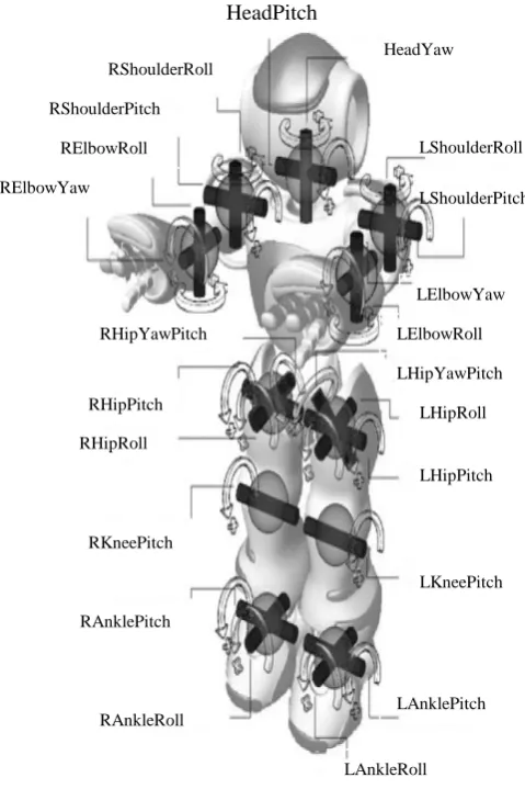
The target Robot of our study is a 22-DOF (degrees of freedom) NAO robot (Fig.1) with 4.5Kg weight and 57Cm stand height. The robot has two arms with four DOF for each arm, two legs with six DOF for each leg and a head with 2 degrees of freedom.
The simulation performed by Rcssserver3d simulator which is a generic three dimensional simulator based on Spark and Open Dynamics Engine (ODE [11]). Spark is capable of carrying out scientific distributed multi agent calculations as well as various physical simulations ranging from articulated bodies to complex robot environments [12]. The time-integrated simulation is processed with a resolution of 50 simulation steps per second. Rcssserver3d simulator is a noisy simulator and to overcome inherent noise of the simulator, Resampling algorithm is implied which could lead to robustness in nondeterministic environments.
Evolution of Biped Locomotion Using Bees
Algorithm, Based On Truncated Fourier Series
Fig. 1 The biped physical structure and its twenty two degrees of freedom. This figure indicates the joint angle and shows the robot coordinate system.
In this approach, the body trunk of the robot is not
actuated. Our experiences show, the leg joints are more
[image:2.595.48.292.605.761.2]effective joints for leg motions, that the joints of hip, knee and ankle which move on the same plane of forward-backward are the major ones (Table 1 shows description of them). Although, other joints are also effective, but in fact, their role smoothes the Robot walking motion. Because of this we prefer to ignore them to decrease learning search space.
TABLE I
MORPHOLOGICAL MAJOR PARAMETERS OF THE NAO ROBOT
Part Joint Name Motion Range
(degree)
Right leg
RHipPitch Right hip joint front and back (Y)
-100 to 25
RKneePitch Right knee joint (Y)
-130 to 0
RAnklePitch Right ankle joint front & back (Y)
-75 to 55
Left leg
LHipPitch Left hip joint front & back (Y)
-100 to 25
LKneePitch Left knee joint (Y) -130 to 0
LAnklePitch Left ankle joint front & back (Y)
-75 to 55
III. JOINT ANGULAR TRAJECTORY
Human motions are recognized flexible and periodic but more challenging for motion stability issue. Therefore, human-like motion patterns are included into the research objectives. The walking trajectory is divided into several types. Positional trajectory and angular trajectory are two of them. The main idea for the walking posture control used here is based on the reaction angular trajectory of the stance leg. Similar to [13] Foot was kept parallel to the ground by using ankle joint in order to avoid collision. Therefore ankle trajectory can be calculated by hip and knee trajectories and ankle DOF parameters are eliminated. Successful walking is defined as an acceptable motion tracking based on the optimized walking [14].
If a gait period divides to equal six time slice, equations (1) and (2) formulate the joint control in the smooth plane. The following notations have been used for variables in the joint angular trajectory formulations:
1. Subscripts 1 and 2 refers to the joint trajectory from the beginning of swing and stand phase respectively. 2. Subscripts h and k denote the hip and knee
respectively.
3. Subscripts l, r, lo refers to left leg, right leg and lock phase respectively.
]
t
,
t
[
θlo
θkr
]
t
,
t
[
θk
θkr
]
t
,
t
[
θkl
θkl
]
t
,
t
[
θlo
θkl
6
4
4
0
1
6
2
2
0
(1)]
6
,
3
[
2
]
3
,
0
[
1
]
6
,
3
[
1
]
3
,
0
[
2
t
t
h
hr
t
t
h
hr
t
t
h
hl
t
t
h
hl
(2)According to equations 1and 2 we can realize that the trajectories for both legs are identical but they have been shifted in time relative to each other by half of the walking period. The joint angle trajectories can be separately looked by ―offsets.‖ The values of the defined offsets actually influence the biped’s posture during walking. Note that in lock phase knee joints only have those offsets for angular trajectory. It can be note that we assume left leg is stand leg in first half period.
IV. TRUNCATED FOURIER SERIES MOTION GENERATOR In equation (3) the original Fourier series of periodic function F(t) has been written
1 2 cos 2 sin 1 0 2 1 ) (i T t
ai and bi are constant coefficients and T is the time period. When i is infinite this formula can produce any complicated signal. But when the value of i is definite, accuracy of signal decrease. Because, walking angular trajectories are too complicated signals, this equation can not create true signals with definite i. Therefore a modified definite Fourier series as a Truncated Fourier series (TFS) has been used as follow:
1
)
sin(
)
(
i
c f
t
i
ai
t
f
(4)Where ai and cf are constants that should be determined and ω is the fundamental frequency determined by the desired period of the gait. n determines the number of terms and can be chosen as a trade-off between the accuracy of the approximation required and the computational load. Note that cf is an offset of angular trajectories that we talked about it before. With this approach and equations of (1) and (2), the TFS for hip-pitch and knee-pitch angles are formulated as follow:
0
,
2
,
)
sin(
)
sin(
2
,
)
sin(
1 1 1 2 1 2 1 1 1
c
c
T
c
t
C
c
t
A
T
c
t
B
k k klo k k k k k n i i k h h h n i i h h h h h h n i i hi
i
i
(5)V. BEES ALGORITHM
Bees Algorithm (BA) which is a nature-inspired algorithm, mimicking the food foraging behavior of swarms of honey bees. It is developed by Pham and et al recently. The BA algorithm is simple in concept, few in parameters, and easy in implementation, it has been successfully applied to various benchmarking and real-world. The algorithm requires a number of parameters to be set, namely: number of scout bees (n), number of elite bees (e), number of patches selected out of n visited points (m), number of bees recruited for patches visited by ―elite bees‖ (nep), number of bees recruited for the other (m-e) selected patches (nsp), and size of patches (ngh). The pseudo code of the BA is as follows:
1: Initialize population with random solutions. 2: Evaluate fitness of the population.
3: While (stopping criterion not met) 4: Select sites for neighborhood search.
5: Recruit bees for selected sites (more bees for better sites) and evaluate fitness.
6: Select the fittest bee from each patch.
7: Assign remaining bees to search randomly and evaluate their fitness.
8: End while
In Step 1, the BA matrix is filled with as many randomly generated solution vectors as the m. Their results calculate in Step 2. In Step 4, bees that have the highest fitness are chosen as ―selected bees‖ and sites visited by them are chosen for neighborhood search. Then, in Steps 5 and 6, the algorithm conducts searches in the neighborhood of the selected sites,
assigning more bees to search near to the best e sites. The bees can be chosen directly according to the fitness associated with the sites they are visiting. Step 7; assign the remaining bees in the population, randomly around the search space scouting for new potential solutions. These steps are repeated until a stopping criterion is met.
VI. APPLYING THE BEES ALGORITHM
With the rule base fixed, the Bees Algorithm was used to tune the parameters of the input and output membership functions and the scaling gains for the input and output variables.
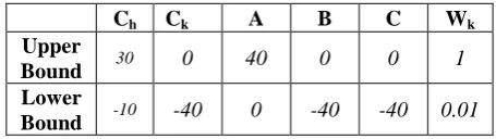
[image:3.595.312.540.341.405.2]In theory, each bee is a vector comprising 6 real numbers. Five of those numbers have been reserved for constant parameters and one has been reserved for the parameter variable of time period. Bees are generated randomly and uniformly for the first iteration between lower and upper bound. In this study the lower and upper bound data for initialization are depicted in Table 2.
TABLE II
LOWER BAND AND UPPER BAND THAT USED FOR HARMONY MEMORY INITIALIZATION
Ch Ck A B C Wk
Upper
Bound 30 0 40 0 0 1
Lower
Bound -10 -40 0 -40 -40 0.01
The following parameter values are set for optimization: population n= 100, number of selected sites m=15, number of elite sites e=5, initial patch size ngh=2 for coefficients and ngh=0.04 for Time period, number bees around elite points nep=10, number of bees around other selected points nsp=3. Note that ngh defines the initial size of the neighborhood in which follower bees are placed.
Fitness function has a critical role in BA and is used to judge how well a solution represented by a Bee is. To achieve more stable and faster walk, a fitness function based on robot's straight movement with having limited time for walking is assumed. The amount of deviation from straight walking is subtracted from the fitness as a punishment to force the robot to walk straight. We ran the simulator for 15 seconds, first the robot is initialized its X and Y values equal to zero and fitness function is calculated whenever robot falls or time duration for walking is over. Equation 6 and 7 show the pseudo code of computing of fitness function in forward and backward walking respectively.
; )
(
; ) (
e CurrentTim on
TimeDurati Y X fitness
len RobotIsFal if
Y X fitness
on TimeDurati e
CurrentTim if
(7)
For computing fitness of backward walking as is shown in equation 7, we multiply the distance that has been passed by negative sign. When robot falls down during walk the fitness is divided to remaining time of simulation. This punishment forces the robot to achieve a stable walk.
VII. RESUALT
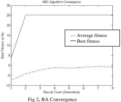
We ran the simulator on a Pentium IV 3 GHz Core 2.6 Duo machine with 4 GB of physical memory, with Linux SUSE 10.3 o.s. The time period for the simulation was 15 seconds. 2 hours after starting BA under the MATLAB, 800 trials were performed. Fig. 2 shows the average and best fitness values during these 8 generations.
Fig 2. BA Convergence
By BA, the robot could walk 4.2 m in 15 s with maximum momentary body speed 0.32. Fig. 3 shows momentary velocity of robot during walk. It can be note that every 50 iteration equal to one second.
[image:4.595.57.256.346.514.2]
Fig. 3: Robot walking momentary velocity. Every 50 iterations equal to one second.
Gait period at the best found fitness equals to 0.42 s. according to this consequence figures 4, 5 and 6, respectively show angular trajectories of hip, knee and ankle, generated by TFS.
[image:4.595.315.521.510.665.2]Fig. 4: left and right hip angle trajectories. Every 50 iterations equal to one second.
Fig. 5: Left and right knee angle trajectories. Every 50 iterations equal to one second.
Fig. 6: Left and right ankle angle trajectories. Every 50 iterations equal to one second.
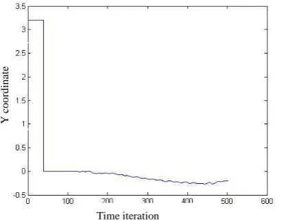
Considerate towards the punishment set for changing direction of robot during movement, Fig. 7 shows the walking direction of the robot
Time iteration
V
el
o
ci
ty
Time iteration
Jo
in
t
A
n
g
le
Time iteration
Jo
in
t
A
n
g
le
Time iteration
Jo
in
t
A
n
g
le
--- Right ankle Left ankle --- Right knee Left knee --- Right hip Left hip
[image:4.595.45.237.591.749.2]Fig. 7: this figure shows Y coordinate of robot during walk. Every 50 iterations equal to one second.
VIII. CONCLUSION
We have demonstrated the suitability of an evolutionary robotics approach to the problem of stable three-dimensional bipedal walking in simulation. The current implementation is capable of walking in a straight line on a planar surface without the use of proprioceptive input. However, in this study for the first time TFS with BA is implemented in a simulated robot that can walk fast and stable. The main advantage of our TFS model is having the least parameters compare with other gait generators models. It is also capable of being implemented on any kinds of humanoid robots without considering its physical model. Using from BA as optimizer shows that The Bees Algorithm is a computationally fast multi-objective optimizer tool for complex engineering multi-objective optimization problems. Resampling technique is also used to overcome uncertainty and noise of the environment.
REFERENCES
[1] Hirukawa H." Walking biped humanoids that perform manual labour," Philos Transact A Math Phys Eng Sci.PMID: 17148050, pp.65-77, 2007.
[2] Vukobratovic M., Borovac B.and Surdilovic. D. ―Zero-moment point proper interpretation and new applications.‖ In: Proceedings of the
2nd IEEE-RAS International Conference on Humanoid Robots, pp. 237—244, 2001.
[3] Zhu C., Tomizawa Y., Luo X. and Kawamura A. "Biped walking with variable ZMP, frictional constraint, and inverted pendulum model", IEEE International Conference on Robotics and Biomimetics, pp: 425-430, Shenyang, 2004.
[4] Kajita S., Kanehiro F., Kaneko K., Yokoi K. and Hirukawa H. ―The 3D linear inverted pendulum mode A simple modeling for a biped walking pattern generation.‖ In: Proceedings of the 2001 IEEE/RSJ
International Conference on Intelligent Robots and Systems, pp. 239– 246, 2001.
[5] Paul C. ―Sensorimotor Control of Biped Locomotion.‖ Adaptive Behavior, vol. 13, no. 1, pp. 67–80, 2005.
[6] Buchli J., Iida F. and Ijspeert A.J. ‖Finding Resonance: Adaptive Frequency scillators for Dynamic Legged Locomotion.‖ In: Proceedings of the 2006 IEEE/RSJ International Conference on Intelligent Robots and Systems. PP. 3903--3910, 2006. [7] Matsuoka K.‖Sustained oscillations generated by mutually
inhibiting neurons with adaptation.‖ Biol. Cybern. 52, 367—376, 1985.
[8] Yang, L., Chew, C.M., Poo, A.N. (2006). Adjustable Bipedal Gait Generation using Genetic Algorithm Optimized Fourier Series
Formulation. Proceedings of the 2006 IEEE/RSJ International Conference on Intelligent Robots and Systems, 4435-4440 [9] Yang L., Chew C. M., Zielinska T. and Poo A. N. ―A uniform biped
gait generator with off-line optimization and on-line adjustable parameters.‖ Robotica 25(5), 549–565, 2007.
[10] Pham D.T., Ghanbarzadeh A., Koc E., Otri S., Rahim S. and Zaidi M. ―The Bees Algorithm, A Novel Tool for Complex Optimisation Problems.‖ Proc 2nd Int Virtual Conf on Intelligent Production Machines and Systems (IPROMS 2006). Oxford: Elsevier, pp. 454-459, 2006.
[11] Smith, R.: Homepage of Open Dynamics Engine project
http://www.ode.org.
[12] Boedecker J.‖Humanoid Robot Simulation and Walking Behaviour Development in the Spark Simulator Framework.‖ Technical report,
Artificial Intelligence Research University of Koblenz (2005) [13] Kagami, S., Mochimaru, M., Ehara, Y., Miyata, N., Nishiwaki, K.,
Kanade, T., Inoue, H. ‖Measurement and comparison of humanoid H7 walking with human being.‖ Robotics and Autonomous Sys. vol. 48, pp. 177—187, 2003.
[14] L. Yang, C. M. Chew, T. Zielinska and A. N. Poo, ―A uniform biped gait generator with off-line optimization and on-line adjustable parameters,‖ Robotica 25(5), 549–565 (2007).
Time iteration
Y
c
o
o
rd
in
at
[image:5.595.56.263.59.220.2]