Abstract—The aims of this paper is to introduce the IEEE 754 standard for the formal method B by introducing the floating-point numbers. We first introduce the four different rounding modes for B method and then we introduce the four essential arithmetic operations, i.e addition, subtraction, multiplication and division for this method.
Index Terms—Abstract Machines, AMN, Formal method, IEEE 754, VDM
I. INTRODUCTION
HE B Method is a formal specification method based
around Abstract Machine Notation (AMN in short) which allows for highly accurate expressions of the properties required by specifications. Recall that formal methods consist of writing formal descriptions, analyzing those descriptions and in some cases producing new descriptions for example refinements from them.
T
The B-Method is a set of mathematically based techniques for the specification, design and implementation of software components. Systems are modeled as a collection of interdependent Abstract Machines, for which an object-based approach is employed at all stages of development. An Abstract Machine is described using the Abstract Machine Notation (AMN). A uniform notation is used at all levels of description, from specification, through design, to implementation. AMN is a state-based formal specification language in the same school as Vienna Development Method (VDM) and Z method. An Abstract Machine comprises a state together with operations on that state. In a specification and design of an Abstract Machine the state is modeled using notions like sets, relations, functions, sequences. The operations are modeled using Pre- and Post-conditions using AMN. One can then prove in a fully automated fashion that these properties are unambiguous, coherent and are not contradictory. This allows us to mathematically prove that these properties are taken into account as the design stages progress.
The formality of the description allows us to carry out rigorous analysis. By looking at a single description one can determine useful properties such as consistency or deadlock-freedom. By writing different descriptions from different points of view it is possible to determine important properties such as satisfaction of high level requirements or correctness of a proposed design. However, this formal specification can only use a set of natural numbers and no
Manuscript received January 14, 2011; revised February 28, 2011. This work was supported in part by the ANR-MUSCADE project and SAFECODE-INRETS project.
H. Ait Haddou is with the National School of Architecture LRA Toulouse and National Institute for Transport and Safety Research, 83 Rue Aristide Maillol, 31100 Toulouse, France (phone: +33-612-935-941; fax: +33-562-115-049; e-mail: [email protected]).
floating-point numbers yet. Therefore, introducing the IEEE 754 standard for B method is very interesting by introducing different rounding modes and the four essential arithmetic operations.
In this paper, we use the representation of floating point numbers in a computer to introduce the IEEE 754 standard for B method. We also prove how rounding can be performed and how limited error is induced to limited precision with operations like addition, subtraction, multiplication and division. The importance of the rounding is illustrated by the Patriot Missile failure [2]. The cause was an inaccurate calculation of the time since boot due to computer arithmetic errors.
This paper is organized as follows. Sections II and III describe the representation and specification of floating-point numbers. Section VI presents a formal description of how floating-point numbers are used to approximate real numbers. We also introduce the four different rounding modes for B method. In section V, we introduce the four essential arithmetic operations, i.e addition, subtraction, multiplication and division for B method.
II.REPRESENTATION
A. Floating-Point Number
The floating-point numbers [3] can be represented as follow: x = s.m.βexp
where s denotes the sign of x (s2
∈
{−1, 1}), β is thefloating-point base (usually 2 or 10), m is called the mantissa, also known as the significand, and exp is the exponent of x.
For example, the floating-point number (fpn) 3.1416 can be written on the floating-point base 10 and precision 5 as . 31416.101, or 314.16.10-2.
As it ca be seen, the definition of exponent is not intrinsic since it depends on the choice of the value of mantissa.
The mantissa m generally composed at least p digits in the base β and p is then called the precision of x. The exponent field exp lies between the maximum and minimum exponent, i.e expmin ≤ exp ≤ expmax.
Once the mantissa is fixed to be an integer, we then have 0 < m < β p, and the computation of floating-point numbers
can be reduced to computation of mantissa as a single integer.
Therefore, to represent a floating-point number, we must clearly define the constants described before. Throughout, we will adopt the following notations:
• exp refers to exponent; • frac: refers to mantissa;
• wordsize: refers to the word size. By definition
wordsize = expsize + fracsize + 1.
• expmax and expmin refer to the maximum and the
Introduction to Floating-Points Arithmetic in B
Method
minimum of exponent respectively.
Remark that the set of all floating point numbers is defined as an abstract set.
B. The FPN MACHINE
The main purpose of this part is to introduce what we call the FPN machine. This machine contains the set of all floating-point numbers. In other words, this set will play the same role as BIG introduced by Abrial in the [1].
In our case, this set will contain the subset fpn of floating described in the beginning. Namely, the set of all floating
x = s.m.βexp. Once this set is defined, we can establish the
restriction relation which asserts for any floating- point in fpn the exponent, sign and mantissa. These functions are well defined and all arithmetic operations remain valid in this case.
Now, let x
∈
FPN, then x is in the form x = s.m.βexp andconsider the three functions define as fellow:
fexp: FPN → NAT
x → exp(x); ffra: FPN → NAT
x → frac(x); fsign: FPN → {0, 1}
x → sign(x).
These three partial functions are well defined and the first important property of each function is that the pair (x, f*(x))
is a member of the function f, provided x is a member of the domain of fi where i
∈
{sign, fra, exp}.III.SPECIFICATION
The standard IEEE 754 specifies four floating-point formats in two groups, basic and extended, with a "single-precision" and a "double-"single-precision" format in each of the two groups.
A. Single Precision
The IEEE single precision floating point standard [4] representation requires a 32 bit word, which may be represented as numbered from 0 to 31. The first bit is the
sign bit, s, the next eight bits are the exponent bits, exp, and the final 23 bits are the fraction frac. In this case, the format is illustrated on table I below.
Single
exp = 8
∧
wordsize = 32.The simple extended precision floating point is given by this relation:
Simple-Extended
exp≥ 11
∧
wordsize ≥43. B. Double PrecisionThe IEEE double precision floating point standard representation requires a 64 bit word, which may be represented as numbered from 0 to 63. The first bit is the sign bit, s, the next eleven bits are the exponent bits, exp, and the final 52 bits are the fraction frac.
Double
exp = 11
∧
wordsize = 64.Similarly, we have the following description for the double extended precision of floating:
Double-Extended
exp ≥ 15
∧
wordsizege = 79.For instance, in single format, the values of constants are
exp=8, frac=23, wordsize=32, expmin=0, exp max=28−1.
In this case, the sign, exponent, and mantissa can be encoded as a single integer. Namely, one have
sign
∈
{0, 1} and exp, frac∈
N. The table II below shows the layout for single (extended) and double (extended) precision floating-point values:TABLE II
IEEE 754 FLOATING-POINT FORMATS
Format Single ExtendedIngle- Double Extended
Double-Expmax +127 1023 +1023 +16383
Expmin -126 1022 -1022 -16382
Exp Bias +127 +1023 +1023 +16383
Precision(bits) 243 32 53 64
Total Bits 3 43 64 80
Sign Bits 1 1 1 1
Exp Bits 8 11 11 15
Frac 23 32 52 64
C. Special Values 1. Zero
Zero is a special value denoted with an exponent field of zero and a fraction field of zero. Note that −0 and +0 are distinct values, though they both compare as equal.
2. Denormalized
If the exponent is all 0s, but the fraction is non-zero (else it would be interpreted as zero), then the value is a denormalized number. Thus, this represents a number
(−1)s × frac × 2 − 126.
For double precision, denormalized numbers are of the form
(−1)s × frac × 2 − 1022.
From this we can interpret zero as a special type of denormalized number.
3. Infinity
The values + and - are characterized by an exponent equal to expmax and a null mantissa.
expmax
∧
frac = 0.4. Not a Number
The value NaN (Not a Number) is used to represent a value that does not represent a real number. NaN’s are represented by a bit pattern with an exponent of all 1s and a non-zero fraction.
In the B method we can describe them as
frac = 0
∧
exp = expmax = 2exp − 1.The table III summarizes the special values.
IV. ROUNDING
The purpose of this section is to present a formal description of how floating-point numbers are used to approximate real numbers.
Floating-point numbers are represented in computer hardware as base 2 (binary) fractions. For example, the
decimal fraction 0.125 has value
10005
1002
101
+
+
, and inthe same way the binary fraction 0.001 has value
8 1 4 0 2
0
+
+
. These two fractions have identical values, theTABLE I
UNITSFOR MAGNETIC PROPERTIES
Sign Exponent Fraction
only real difference being that the first is written in base 10 fractional notation, and the second in base 2.
Unfortunately, most decimal fractions cannot be
represented exactly as binary fractions. As a consequence, generaly the decimal floating-point numbers you enter are only approximated by the binary floating-point numbers actually stored in the machine.
The problem is easier to understand at first in base 10.
Consider the fraction
3
1 . You can approximate that as a
base 10 fraction: 0.3 or, 0.33 or, better, 0.333 and so on. No matter how many digits you are willing to write down, the
result will never be exactly
3
1 , but will be an increasingly
better approximation of
3
1 .
In the same way, no matter how many base 2 digits you are willing to use, the decimal value 0.1 cannot be represented exactly as a base 2 fraction.
Because of the finite precision of floating-point numbers, floating-point arithmetic can only approximate real arithmetic. Every floating-point number is a real number, but few real numbers have floating-point equivalents. Consequently, floating-point operations (addition, multiplication, division, etc.) are generally thought of as being composed of the corresponding real operation followed by a rounding step which chooses a floating-point number to approximate the true result.
A. Definition of function ulp
There are several different definitions of function ulp, see for instance [5]- [6]. In this work we restrict ourselves to the original definition due to W. Kahan in 1960 [8]. The term ulp is an acronym for unit in the last place and the original definition is: ulp(x) is the gap between the two floating-point numbers nearest x, even if x is one of them. As told by Kahan [8], the adoption of the IEEE-754 standard for floating-point arithmetic has made infinities and NaNs
ubiquitous, and that must be taken into account in the definition of ulp(x). Kahan now suggests the following definition: ulp(x) is the gap between the two finite floating-point numbers nearest x, even if x is one of them. (But
ulp(NaN) is NaN.). In other words, the KahanUlp (x) is the width of the interval whose endpoints are the two finite representable numbers nearest x (even if x is not contained within that interval). The table IV below summarizes the IEEE 754 standard bounds.
In this paragraph, we recall some properties of the function ulp(x) regarding different rounding modes.
Property 1 Let X be a flouting point number and x a real number. Then, with rounding to nearest (RN) and in radix 2, one have
|X − x| <
2
1 HarrisonUlp(x)X = RN(x)
Note that this property is not true with radices greater than or equal to 3. The following counter-example in radix 3 explain this situation.
Let X = 1- = 1 – 3-n and take x such that 1< x <1 +
2
1 3
-n. Then HarrisonUlp(x) = 3-n+1, and |x−X| <
2
3−n+1 , so that
|x−X| < 21 HarrisonUlp(x). But X ≠RN(x).
The following property is proved for any radix:
Property 2 Always with rounding to nearest (RN), one have
X = RN(x) |X − x| <
2
1 HarrisonUlp(x)
Property 3 For any radix and with rounding to nearest (RN),
|X − x| <
2
1 KahanUlp(x)X = RN(x)
Property 4 In radix 2,
X = RN(x) |X − x| < 21 KahanUlp(x)
Let 1 – 3-n < x < 1 + 3-n, then RN(x) = 1 and
|x − 1| >
2
1 KahanUlp(x).
This example shows that the previous property is not true in radix 3.
Remark that with rounding to nearest in radix 2, both Kahan’s and Harrison’s definitions preserve the common claims listed above.
B. Rounding modes
The IEEE standard has four different rounding modes; the first is the default; the others are called directed rounding.
1. Round to Nearest rounds to the nearest value; if the number falls midway it is rounded to the nearest value with an even (zero) least significant bit, which occurs 50% of the time (in IEEE 754r this mode is called roundTiesToEven to distinguish it from another round-to-nearest mode)
2. Round toward 0 directed rounding towards zero
3. Round toward + directed rounding towards positive infinity
4. Round toward − directed rounding towards negative infinity.
For the IEEE standard double precision (frac = 52), numbers x
∈
(1, 1+2-frac) are rounded to:• 1 if 1 < x _ 1 + 2-52
• 1 + 2-52 if 1 + 2-52 < x < 1 + 2-52
For all but specifically designed numerical analysis applications, round to nearest is the best rounding mode. In
TABLE III TABLEOFSPECIALVALUES
Name exp frac sign expbits fracbits
+0 min-1 0 + 0000000 0000000
-0 min-1 0 - 0000000 0000000
Number min≤e≤max any any any any
+ max+1 0 + 1111111 0000000
- max+1 0 - 1111111 0000000
NaN max+1 0 any 1111111 any
TABLE IV IEEE 754 STANDARDBOUNDS
Single Double
Exp bits 8 11
Frac 23 52
round-to-nearest mode, the nearest representable value is never more than 1/2 ULP away from the exact result being rounded, so the error introduced by rounding is never more than 1/2 ULP. For the other rounding modes, the error is less than 1 ULP.
As an example of the size of a 1/2 ULP rounding error: suppose you tried to measure precisely the distance to the sun (about 149.63700 million kilometers, see table V).
An error of 1/2 ULP in single-precision would put your measurement off by about 232.5 kilometers; an error of 1/2 ULP in double-precision would put it off by about 8 microns; and an error of 1/2 ULP in quad-precision would put it off by about 10-17 microns, which is about one millionth of the diameter of a proton.
Let x be the exact value of any given operation, and x−, x+ two floating points such that x− ≤ x ≤ x+.
The rounding towards negative infinity is x−, to positive infinity x+, rounding to zero is x− if x ≥ 0, and x+ if x < 0. Rounding to the nearest is defined as the number of x− and
x+ which is closest to x, in the event of a tie, this is the case when x is in the middle of two floating numbers, the IEEE standard imposes choose one with an even mantissa.
C. Exactly rounded
The important consequence of rounding is the fact that once the rounding mode is chosen, the result of any operation is perfectly specified, especially when the result is unique. We then tell about the exactly rounded also called correctly bounded.
The IEEE standard 754 imposes the exactly rounded for the four basic arithmetic operations (addition, subtraction, multiplication and division) and square root. Thus, a program using these five operations behaves the same way on any configuration respecting the IEEE 754 standard, provided there are no intermediate precision and that the
programming language does not allow the compiler to change operations if it can produce a different result.
The exactly rounded property allows building proved algorithms using these five basic operations (TwoSum, FastTwoSum, Sterbenz, Dekker, see for instance [9]).
The directed rounding toward positive or negative infinity allows carrying out interval arithmetic [11], i.e. to calculate for every operation an upper or a lower bound to the exact value. We do not need the exactly rounded to do this, the respect of the definition of rounding suffices, but the correct rounded gives the best possible result. On the other hand, the IEEE 754 standard imposes nothing for the other mathematical operations (power, exponential, logarithm, sinus, etc.) for which no requirement is imposed.
Since real numbers are not yet directly used in B, as we need to prove properties for both abstraction and
implementation. Real numbers being implemented on all computers as approximations, we could find combination of operations that would behave differently as abstraction and as C code implementation, because of numerical erosion. Instead, we manipulate big integer numbers. For example, if we want to represent a speed varying between 0 à 5m/s with
a 0.01 m/s accuracy, define a [0, 500] interval, 0 representing 0 m/s, 500 for 5.00 m/s.
The following theorem, due to Nesterenko-Waldschmid [10], was used to show that getting exactly rounded results in double precision could be done with frac _ 1000000. Remember that computing functions with 1000000 digits is feasible.
Theorem 1 (Y. Nesterenko and M. Waldschmidt (1995)) Let p/q, r/s be rational numbers, with p ≠ 0 and A, B and
E be positive, real numbers with E ≥ e satisfying
A≥ max (max (p, q), e), B ≥ max(r, s).
Then
|e r/s –p/ |≥ exp(−211 × (logB + loglogA + 2log(E|r/s| +) +
10)x (logA + 2E|r/s|+6logE)×(3.3log(2) + logE)×(logE)-2)
where |r/s |+ = max(1, |r/s |).
D. Double Rounding
Let x be a real number, y the rounding of x in p precision and z the rounding of y in precision q < p. Then, z is not always the rounding of x in precision q.
For example, in the case of round to nearest, x = 1.0110100000001 rounded to 9 bits gives y = 1.01101000, which rounded to 5 bits gives z = 1.0110 while the direct rounding of x to 5bits gives z’ = 1.0111. We call this the problem of double rounding.
On x86 architectures, when the three variables are double precision floatingpoint numbers, to compute c = a + b, by default, two successive roundings will occur:
1. First in extended precision during the addition,
2. Then in a lower precision when storing the value into memory.
In most cases, the final result is the correct rounding of the sum of the two floating-point numbers, but not always.
E. Round-to-nearest-even and round-to-nearest modes
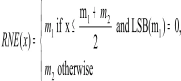
Let x be a fractional number between two consecutive representable fractional numbers m1 and m2 such that
m1≤ x < m2. Let denote by RNE the round-to-nearesteven mode and LSB(mi) represents the least significant bit of mi where i
∈
{1, 2}.The RNE mode rounds x to the nearest representable number. When x is exactly in the half way between two representable numbers (tie case), it is rounded to the nearest even number. RNE is expressed as
≤
+
=
=
otherwise
,0
)
LSB(m
and
2
m
x
if
)(
2
1
2
1
1
m
m
m
x
RNE
The round-to-nearest mode RN is similar to RNE, except for the handling of a tie case. When a tie case occurs, RN unconditionally rounds the number up. RN is expressed as
+
=
otherwise
,
2
m
xif
)(
2
2
1
1
m
m
m
x
RN
[image:4.595.315.496.561.642.2]For the basic floating-point multiplication algorithm, both
TABLE V
EXAMPLEOFTHEASIZEOFA ½ ULPROUNDINGERROR
Distance 1/2ulp rounding error
km 149.637000 232.5
RN and RNE can be performed by first adding 2-n to the normalized product, and then discarding the n less significant bits of the normalized product. If RNE is performed, the previously added 2-n should be subtracted when the tie case occurs and the nearest-up number is odd. This correction can be made by complementing the least significant bit of the rounded product.
F. Rounding errors
The major problem of floating is the propagation of rounding errors due to the problem of “cancellation”, the final result of any computation including several operations may be far from the true value, even if in some cases, in the opposite sign sign.
The Rump two-variate polynomial constitutes an example to illustrate the rounding error problem:
R(x,y)=1335y6/4+x2(11x2y2 – y6 − 121y4 − 2) +11y8/2+ x/2y
We want to find the sign of R(77617, 33096). Since it is impossible to stop the propagation of rounding errors, it is important to bound the final error. To do this, one can bound the absolute error, the relative error, or bound error on ulps.
Absolute error
The absolute error is generally used when the upper bound of the intermediate values are known. For example, lets compute the following sum: S = t1 + t2 + ... + tn, such
that the intermediates are bounded in absolute value by α, then each partial sum give rise to a rounding error less than
1/2 ulp(α) using rounding to nearest mode. The final error is then less than (n−1/2) ulp(α).
Relative error
The relative error is used, when the boundary of intermediate values. Let * be a mathematics operator, and for any real numbers a and b we denote by RN(a*b) the correct rounding of a*b. In this case, Highan [7] shows that the final relative error of this operation c = RN(a*b) is (1+β)n−1 where β is such that c = (1+β)(a*b).
V.ARITHMETICOPERATION
A. Addition, subtraction, multiplication and division
The four essential arithmetic operations are addition, subtraction, multiplication and division. In this work, we denote by OP the set of these four operations (add, sub, mul, div), namely,
OP =:: add | sub | mul | div.
A floating point arithmetic is a mapping which assigns for each pair of floating point numbers x and y and each op
∈
OP another floating point number, denoted op(x, y),provided y≠0 when op = div.
The basic floating-point multiplication algorithm is described as follow:
Let (s1, frac1, exp1) and (s2, frac2, exp2) be representation
of two floating-point numbers. The multiplication of these two representations gives an approximate result (sp, fracp,
expp) with no regard to rounding. This means that their
mantissas are multiplied, their exponents are added, and their sign bits are XORed. The intermediate results are sent to the round, which rounds according to the mode and destination format as detailed in the previous section. Observe here that the multiplication stage was decomposed into operations on the mantissa, exponent and sign. These three constants are natural numbers and all basic operations in this set are already defined for B method.
Using the two representations above, we verify the following properties of the mantissa, exponent and sign computation:
signp = sign1 × sign2
expp = exp1 + exp2 + p + bias;
where p represents the number of bits in the fraction.
fracp + 1 > frac1 × frac2
fracp≤ frac1 × frac2.
The division and square root are more difficult to specify and verify than the multiplication, addition and subtraction. This difficult comes from the fact that the result of these operations are rational or irrational number.
By using same notations of multiplication one can prove that sign1/sign2= sign1 × sign2.
Let x and y be two floating point numbers and denote by op(x, y) the results of the operation op
∈
OP. Then, we have the following inequalities:wordsizeop (x,y) ≥ wordsizex and wordsizeop (x,y) ≥ wordsizey.
Remark that if x = 0 and y≠ 0 the result div(x, y) is a NaN. Similarly, sub(+∞,+∞) = NaN.
The floating point subtraction is anti-symmetric if
op(x − y) = −op(y − x) for all x and y.
It is monotonic if x ≤ y implies op(x − z) ≤ op(b − z) for all
z. Furthermore, subtraction can fail to be anti-symmetric in IEEE standard arithmetic only when a rounding mode other than the default is used.
Note also that in arithmetics with signed zeros, the computed value op(x−x) can differ from the computed value
op(−op(x − x)), but the numeric value y of the result of
op(x − x) still satisfies y = −y, and this latter property suffices to satisfy anti-symmetry.
Anti-symmetry
op(x − y) = −op(y − x) op(x − x) = op(−op(x − x))
Monotony
x ≤y op(x − z) ≤op(b − z) for all z. B. Square Root Implementation
In this part we restrict ourselves to single-precision floating point numbers. To compute square root with correct rounding, we first need to handle special values, i.e zero, infinities, NaNs. For these special values, the B machine respects some known properties of the square root function. Therefore, for any floating point number x one have:
{
+ − +∞}
∈
∀x 0, 0, x = x
x= NaN for x < 0 and x = −1.
Once the square root for special values is specified, we now consider a floatingpoint number x unpacked in three fields, sign, fraction and exponent, like in section 1.
Let x be a normalized single-precision floating-point number and x = sign.frac.2exp with exp an integer between
-126 and 127.
Since the square root number of floating point is a floating point number and it is always positive, then the sign can be ometed and the decomposition of x can be written as
x= l.2d,where d = exp/2 , l = t frac and t=1 or 2
depending on the parity of exp. Remark here that exp needs not be incremented.
Suppose that the fraction frac has the binary expansion
frac = ±1. f1 f2 …f23, then to compute the exact value of x
, under round-to-nearest rounding, reduces to computing the exact values of the bits l1l2...l 23l 24... where l1l2...l 23l 24... is
Newton-Raphson method
The purpose of Newton-Raphson method is to find approximations of zeros of differentiable functions. In this section, the Newton-Raphson’s method is used to approximate the square root function.
Several floating-point divide and square root algorithms are based on the Newton-Raphson iterative method and on polynomial evaluation. For example if we want to compute s
t the Newton-Raphson method is used, a number of iterations first calculate an approximation of 1/t , using the function f(x) = t −1/x.
Take an arbitrary floating-point number x0 and define by
iteration xnas follow: xn+1 = xn – (f(xn)/f’(xn))
Here, f’ denotes the derivative of the function f.
The initial value x0 can be chosen, in the absence of any
intuition about where the zero might lie, by using the intermediate value theorem.
Example Let a be a positive real number. We want to compute, using the Newton-Raphson method, the square root of a. To do this, let define the function f(x) = x2 − a.
The zero of this function is exactly the square root of a. Newton-Raphson’s method starts with a guess x0 and
iteratively refines this guess.
C. Exact floating point computation
The exact rounding allows proving properties for floating point system and devising algorithms to make exact calculation using the floating as building blocks.
We consider here a system with the base 2, and a mantissa with p bits. We also consider the rounding to nearest mode, even if some results are generally true for any base.
Let denote by⊕, Θand ⊗the three arithmetic operations addition, subtraction, multiplication respectively with respect to correct rounding.
Correct Rounding (IEEE 754):
a⊕ b = p (a + b); aΘb = 0
⇒
a=b.The computed value a⊕b or aΘb is exact when
a⊕ b = a + b and aΘb = a − b.
Sterbenz theorem
Theorem 2: Let x and y like signed-machine numbers and, without loss of generality, assume that both x and y are positive. Suppose that y/2≤ x≤2y. If subtraction is performed with a guard digit, and underflow does not occur, then the computed value xΘy of x − y is exact.
We now consider a general property known as faithfulness. This property is very useful to prove the correctness of many computations.
For floating point numbers x and y and op
∈
{add,mul, sub, div}, let z = op(x, y) exactly such that y ≠ x if op = div. Let s and t be consecutive floating point numbers with the same sign as z, such that s ≤z <t . Then the floating point arithmetic is called faithful if op(x, y) = swhenever
z = s and op(x, y) is either s or t whenever z≠ x.
As a consequence of this definition, we give this lemma:
Lemma If a and b are floating point numbers with mantissa t and basis α such that 1/2≤a/b≤2, then a−b is also a floating point number with mantissa t and bias α. In particular, in a faithful arithmetic, op (a − b) = a − b
exactly.
VI. CONCLUSION
Formal methods are a particular kind of mathematically-based techniques for the specification, development and verification of software and hardware systems. The use of formal methods for software and hardware design is motivated by the expectation that, as in other engineering disciplines, performing appropriate mathematical analysis can contribute to the reliability and robustness of a design. However, the high cost of using formal methods means that they are usually only used in the development of high-integrity systems, where safety or security is of utmost importance. This paper presents the IEEE 754 standard for B method by introducing the floating-point numbers. We first introduced the four different rounding modes for B method and then we have introduced the four essential arithmetic operations. This work will surely enable the B-tool software to handle real numbers and thus increase the scope of this formal method to cover more complex projects that developers could not modelize by using only integers.
REFERENCES
[1] J. R. Abrial. The B Book: Assigning Programs to Meanings. Cambridge University Press New York, 1996.
[2] D. N. Arnold (1988). Some disasters attributable to bad numerical computing. Cambridge University Press [Online]. Available: http://www.ima.umn.edu/ arnold/disasters/.
[3] W. D. Clinger. “How to read floating point numbers accurately,” ACM PLDI, 1990 pp. 92–101.
[4] D. Goldberg. “Eee standard for binary floating-point arithmetic,” New York: ANSI/IEEE, Std. pp. 754-785, 1985.
[5] D. Goldberg. “What every computer scientist should know about floatingpoint arithmetic,” ACM PLDI, vol 23, no 1, 1991.
[6] J. Harrison. A machine-checked theory of floating-point arithmetic. Lecture Notes in Computer Science, 1999.
[7] J. L. Boulanger and G. Mariano “Formal modeling of digital circuits using the B method,” Research rapport, INRETS-ESTAS, 1999. [8] W. Kahan. A logarithm too clever by half. ., 2004.
[9] D. E. Knuth. The art of computer programming. Addison-Wesley, 1973. vol. 2.
[10]Y. V. Nesterenko and M. Waldschmidt. On the approximatio, of the values of exponential function and logarithm by algebraic numbers. Mat. Zapiski, 1996.