Elastoplastic Large Deformation Using Meshless Integral Method

Elastoplastic Large Deformation Using Meshless Integral

Method

Jianfeng Ma1, X. J. Xin2

1_{Department of Aerospace and Mechanical Engineering, Saint Louis University, Saint Louis, USA} 2_{Department of Mechanical and Nuclear Engineering, Kansas State University, Manhattan, USA}

Email: [email protected], [email protected]

Received September 23, 2012; revised October 24, 2012; accepted November 4, 2012

ABSTRACT

In this paper, the meshless integral method based on the regularized boundary integral equation [1] has been extended to analyze the large deformation of elastoplastic materials. The updated Lagrangian governing integral equation is ob- tained from the weak form of elastoplasticity based on Green-Naghdi’s theory over a local sub-domain, and the moving least-squares approximation is used for meshless function approximation. Green-Naghdi’s theory starts with the addi- tive decomposition of the Green-Lagrange strain into elastic and plastic parts and considers a J2 elastoplastic constitu-

tive law that relates the Green-Lagrange strain to the second Piola-Kirchhoff stress. A simple, generalized collocation method is proposed to enforce essential boundary conditions straightforwardly and accurately, while natural boundary conditions are incorporated in the system governing equations and require no special handling. The solution algorithm for large deformation analysis is discussed in detail. Numerical examples show that meshless integral method with large deformation is accurate and robust.

Keywords: Meshless Method; Large Deformation; Local Boundary Integral Equation; Moving Least-Squares Approximation; Subtraction Method; Singularity Removal; Elastoplasticity; Green-Naghdi’s Theory

1. Introduction

Over the past two decades the meshless methods have attracted much attention owing to their advantages in adaptivity, higher degree of continuity in the solution field, and the capability to handle moving boundaries and changing geometry. In the meshless method, the concept of an element is eliminated. The model geometry consists of a distribution of nodes over the problem domain, and the approximate solution is constructed entirely based on these nodes. Most development in meshless methods to date has been focused mostly on linear elasticity. Re- search in large deformation plasticity using meshless methods is only currently gaining attention.

For the formulation of elastoplastic theory at large de- formation, Green-Naghdi’s theory [2,3] begins with the additive decomposition of the Green-Lagrange strain into elastic and plastic parts as e p

KL KL KL

E E E . On the other hand, Lee’s theory [3,4] considers the multiplica- tive decomposition of deformation gradient F into an elastic Fe _{and plastic part F}p _{as F F F}e p_{. Both theo-} ries are formulated on the basis of fundamental laws of continuum mechanics. According to Chiou et al. [3], Green-Naghdi’s theory is more flexible because it can be applied to either isotropic or anisotropic materials and the computing procedure involved is relatively straight-

forward. In general, theories of large deformation plas- ticity have to be implemented numerically since it is dif-ficult to obtain closed form solutions to practical prob- lems involving large deformation. Researchers such as Chiou etal. [5], Lee [6], and Hu [7], have used FEM to solve large deformation plasticity problems.

approximation to construct shape function. The system equation is obtained based on the Total Lagrangian (TL) approach. Hu et al. [13] used meshless local Petrov- Galerkin method for large deformation contact analysis of elastomeric components. A nonlinear formulation of meshless local Petrov-Galerkin finite-volume mixed me- thod was developed by Han et al. to analyze static and dynamic large deformation problems [14]. Li etal. [15] developed a coupled finite element and meshless local Petrov-Galerkin method to analyze large deformation problems. Gu et al. [16,17] employed meshless local Kriging method to analyze large deformation problems. A comparison between Total Lagrangian and Updated Lagrangian approaches with an adaptive local meshless formulation was given by Gu in [18]. Gun et al. [19] used a meshless formulation of the Euler-Nernouli theory with non-linear strain-displacement relation which covers both axial and bending deformations to predict the large deformation behavior of fabrics. Li and Lee [20,21] em- ployed an adaptive meshless method to solve mechanical contact problems which incorporated a sliding line algo- rithm with penalty method to handle contact constrains. In [22], Zhu etal. used meshless local natural neighbor interpolation method to analyze 2D elastoplastic large deformation in conjunction with Updated Lagrangian formulation. A Galerkin SPH method was utilized by Wang to solve large deformation fracture problems [23]. Reproducing kernel particle methods were used to ana- lyze large deformation problems in [24-26]. In [27], Li et al. used an element-free Galerkin method to solve die forging problems. Quak etal. [28] applied both SPH and EFG meshless methods to analyze extraction problems.

The authors have developed a meshless integral method for linear elasticity [1] and later extended it to elastoplas- ticity for small deformation [29]. This meshless integral method is truly meshless and does not require a back- ground mesh for integration. In the present work, we extend the meshless integral method to large deformation elastoplasticity. The governing integral equation is ob- tained from the weak form based on Green-Naghdi’s large deformation elastoplasticity theory over a local sub- domain, and moving least-squares approximation is used for meshless function approximation. The constitutive law uses A J2 elastoplastic flow theory based on von

Mises yield criterion with isotropic hardening in which the Green-Lagrange strain is related to the second Piola- Kirchhoff stress. The fixed point iteration, because of its simplicity in implementation, is used to solve the nonlin- ear equations arising from large deformation elastoplas- ticity. A number of numerical tests were carried out for model verification. It was found that the meshless results are in excellent or satisfactory agreement with either closed form solutions or FEM results, indicating that the large deformation elastoplasticmeshless integral method

based on the regularized integral equation is accurate and robust. An application of the current method to the metal forming process has been reported separately [30].

This paper is organized as follows: In Section 2, the regularized local boundary integral equation is derived, and the subtraction method is used to remove the strong singularity that is present in the initial local boundary integral equation. In Section 3, large deformation elasto- plastic constitutive equations are presented. Section 4 describes the moving least-squares approximation (MLSA) for approximating the displacement, strain, and stress fields over the problem domain. The meshless imple- mentation of the regularized boundary integral equation using MLSA and the treatment of weak singularity are presented in Section 5. Section 6 discusses the enforce- ment of essential and natural boundary conditions. The solution algorithm for solving the nonlinear system equa- tions is discussed in Section 7. Numerical examples are presented in Section 8 to assess the accuracy and effec- tiveness of the method. Discussion and conclusions from this study are given in Section 9.

2. Regularized Local Boundary Integral

Equation Using Subtraction Method

In this work, the updated Lagrangian coordinate system is used in which the stress directions are referred to the last known equilibrium state. Consider a two-dimen- sional body for a given load increment as shown in Fig-ure 1. The equilibrium state of the body at the beginning of the load step, which has been solved and is denoted by Ω0, is referred to as the referenceconfiguration. The ref-

erence configuration designates the configuration with respect to which subsequent deformation is measured. The domain of the current configuration of the body at the end of the load increment is denoted by Ω, which is also called the deformedconfiguration. The vector X for a given material point in the reference configuration does not change with time, and X is called the Lagrangian coordinates; x, which describes the material point in the current configuration, changes with time, and x is called the Eulerian coordinates. In this work, the rectangular

Eulerian coordinates, xk (k = 1, 2), and Lagrangian coor- dinates, XK (K = 1, 2), are employed. We use upper case letter and upper case subscript to indicate that the vari- able of interest refers to the reference state, and use lower case letter and lower case subscript to indicate that the variable of interest refers to the current state. Within the updated Lagrangian framework, the following proce- dures are implied: 1) During each load increment, all field variables are defined with respect to the state at the start of this load increment (reference configuration); 2) At the end of this load increment, field variables are up- dated with respect to the state at the end of this load in- crement (current configuration), and the current configu- ration will be the reference configuration for the next load increment.

In large deformation problems, various stress measures can be defined. The most commonly used stresses are: 1) Cauchy stress (true stress) tensor σ which expresses the stress relative to the current configuration; 2) First Piola- Kirchhoff stress (nominal stress) tensor P which relates forces in the current configuration with areas in the reference configuration; 3) Second Piola-Kirchhoff stress tensor T which relates forces in the reference configuration to areas in the reference configuration, where the force in the reference configuration is obtained via a mapping that preserves the relative relationship between the force direction and the area normal in the current configuration. The relationships between these stresses are

1 _, 1 T_,

J  J  

    

P F σ T F σ F

where F is the deformation gradient and defined as

x x

X Y

y y

X Y

 

 

_{ } 

  

 

 

_{ } 

 

F , and J is the determinant of F. The

second Piola-Kirchhoff stress tensor is symmetric, and in the current work is linked to the Green-Lagrange strain in the elastoplastic constitutive law.

For a large deformation elastoplastic body represented by a reference domain Ω0 with boundary Γ0, the govern-

ing elastoplasticity equations are as follows:

 

 

 



 

 

 

 



 

 

 

, 0

, , , ,

0

0 1

, 2

Ω

IJ J I

IJ I J J I K I K J

e cor

IJ IJKL KL IJ

f

E u u u u

dT C dE dT

 

  



 _{  }

    

 



X X

X X X X X

X

X X X

(1)

where τ (bold face denotes vectors or tensors) is the

stress measure defined by r

IJ rI rJ rI LJ L

x

G G T

X

    _  _   ,

TLJ is the second Piola-Kirchhoff stress, G is the trans- formation tensor between the reference configuration and

the current configuration, r L

x X



 is the deformation gra- dient, E is the Green strain tensor associated with the displacement u_, ρ0 is the mass density in the reference

configuration Ω0, fI is the body force per unit mass, e

IJKL

C is the linear elastic stiffness matrix, and cor IJ

dT is

the stress correction term because of nonlinearities in either geometry or material. An index I following a comma designates partial differentiation with respect to XI, and repeated indices indicate summation over the dimensionality of the problem. The essential and the natural boundary conditions on the boundary Γ are re- spectively:

on

I I u

u u  (2)

on I IJ J I t

T  n T  (3)

here, u represents the prescribed displacement on u, T represents the prescribed traction on t; n is the outward unit normal to the boundary; _t  _u and

t u    .

The weak form of (1) over a local sub-domain

0 0

a

   in the reference state is:

 

 









 

0

, 0 , d 0 0

a

a IJ J fI gI

 



  



X X X Y X (4)

where the notation  in this paper is used to denote a node (e.g., a indicates node a, b indicates node b, etc.) in order to reserve the usual subscripts, I, J, etc., for denoting degree of freedom (DOF) components,

0 0

a

   is a spherical (circular in 2D) sub-domain related to node a , _Y a _{is the position vector of node} a which is also called a sourcepoint, X is the integration or fieldpoint which may or may not coincide with a node, and gI is the test function. In the following, the func- tional dependence on X, i.e. “(X)”, will be dropped for brevity when no ambiguity is caused. In this work, fol- lowing [31], we use a special test function defined by



, a





, a

  

a

I JI J

g _{X Y }u_ _{X Y} e _{Y (5)} where eJ represents the J-th component of a unit force vector, uJI is the special test function, given by [31]:

















2₂

2

2 2

, 1 8π 1

5 4

4 3 ln 1

2 3 4

1 a IJ

a a

IJ

a a

s s

a a a

I J a a s

u

r v r

v

h h

r r r

h r

 

 







 

 

 _  

 _{  }

  

 _{  }

 

  





  _

 _ _  

  

 X Y

where _ra _{is the distance from Y} a _{to X;} a a

I I I

r X Y ; na is the outward unit normal to the boundary 0

a

 at X; a s

h is the radius of the local sub-domain;   and E E for plane strain, or



1



   and _{E E}



_12



_{for plane stress; E is}

the Young’s modulus,  is the Poisson’s ratio, and







2 1



E

  is the shear modulus. Note that the special test function is defined in the reference state. The associated traction, for linear elastic behavior, is





























2 3 2 2 , 1 1 1 2

4π1 3 4

1 2 2 3 3 4 a IJ a a a K K IJ a a a

s

a a a

a a a a I J

I J J I a a a

a a a a I J J I

a s t r n r v

v r n v h

r r

r v

r n r n

n r r

r n r n

v h    _         _   _           _  _

 _{X Y}

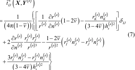
(7)

The special test function u_IJ _{has the property that it}

vanishes on the boundary of a spherical 0 a

 . With uIJ 



as the test function, application of integration by parts to (4) twice leads to:





   





   





   





 

 





 





 

 

 





 



 



 

0 0 0 0 0 0 0 * 0 , , , , 0 , , , d , d , d , d , d , d , d a a a a a a a a I a IJ J a IJ J

a cor r

IJ K LK rJ

L

a e

IJ K RJ R L LKMN M N

a

IJ LK J L K

a

IJ LK JL J L K

u u T t u x u T X

u u C u

u T u n

u T u n

                                       















     

X Y X X

X Y X X

X Y X X

X Y X X

X Y X

X Y X X X

X Y X X X





   

0

0

, d 0

a

a

IJ J

u  f



 



 X Y X X

(8) where 0

a

 is the boundary of 0 a  , 0

J

T is the J-th component of the traction at the reference state, uI _is the displacement increment from the reference state to the current state, 0

LK

T is the second Piola-Kirchhoff stress at the reference state, TLKis the second Piola- Kirchhoff stress increment from the reference state to the current state, and _



_{X Y}, a



_{is the Dirac delta function.}

Equation (8) in its current form cannot be used directly in numerical calculation because when Y a is a boundary node, the equation contains strong singularity (1/r type in line integral) in the traction term tIJ



 _{. For the local inte-}

gral equation approach to be a valid numerical method, the strong singularity must be handled appropriately.

The subtraction technique is employed in the present study to remove the strong singularity; the technique for small deformation has been presented in 4 chosen, in the reference state, as a sphere or part of a sphere centered on a node. If node Y a is an interior node, a

s

h _{is selected such that} 0 a

 stays fully inside

0

 . If _Y a

is a boundary node, then 0 a

 is the in- tersection of 0 and a sphere

a



 of radius a s

h , centered at the boundary node, and the boundary _0a is the union of the part of _a

inside 0, denoted

by _Ca _{, and the part of} 0

 inside _a _{, denoted} by Γa , as illustrated in Figure 2. A further modifica- tion is the exclusion of a tiny sphere  of radius Δ

(which later tends to zero) centered on Y a whose boundary is denoted by _Ca

 . Figure 3 shows sche-

matically this modification. For interior nodes, Γa _is empty, and _Ca _{is a full circle.}

With the above notations, the boundary 0 a

 can be decomposed into the following sections:

0 Γ

a _Ca a _Ca 

    (9)

a a a u t

    (10) where ua is the section of

a

 where the displace- ment is prescribed, and a

t

 the section where the trac- tion is prescribed.

Using subtraction method, we obtain, in the limit of

0

[image:4.595.63.288.203.321.2]

  , the following:

Figure 2. Schematic diagram showing the sub-domain for an interior or a boundary node Ya

[image:5.595.312.534.86.203.2]

Figure 3. Exclusion of a tiny sphere ΩΔ of radius Δ centered

at a node for removing the strong singularity.





 

 





 





 

 

 





 



 



 





   







 



 







 



0 0 0 0 , , , , 0 , , 0 , d , d , d , d , d , d , d a a a a a a

a cor r IJ K LK rJ

L

a e IJ K RJ R L LKMN M N

a

IJ LK J L K

a

IJ LK JL J L K

a IJ J

a a IJ J J C

a a IJ J J

x

u T

X

u u C u

u T u n

u T u n

u T

t u u

t u u

                                     













      

X Y X X

X Y X

X Y X X X

X Y X X X

X Y X X

X Y X X

X Y X

 





   

0

0

, d 0

a

a

a IJ J

u  f

     





 X

X Y X X

(11) The integration of



, a



IJ

t_ _{X Y over C}a _{can be} obtained in closed form:



,



dΓ

a

a a IJ IJ C

t _{ }



 X Y (12)

with

















2 1 2 1

2 1 2 1

sin 2 sin 2 cos 2 cos 2

2π 2π 3 4 2π 3 4

cos 2 cos 2 sin 2 sin 2

2π 3 4 2π 2π 3 4

a IJ                      _{ }   _{ }                    (13)

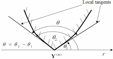
Here  2 1  is the internal boundary angle sub-

[image:5.595.58.288.86.231.2] [image:5.595.58.293.266.696.2]

tended by material at Y a on the boundary, as shown in

Figure 4.

Figure 4. Schematic diagram showing the internal bound- ary angle θ2 – θ1 = θ at node Ya on the boundary.

Several special cases are worth noting. For an interior node,  2π; for a boundary node where the boundary is smooth,  π; for a corner node, θ = corner angle.

Substituting the above expressions into (11) leads to:





 

 





 





 

 

 





   





   





 



 



 

0 0 0 0 0 , , , , 0 , 0 0 , , d , d , d , d , d , d a a a a a a u t a

a a a cor r IJ J IJ K LK RJ

L

a e IJ K RJ R L LKMN M N

a

IJ LK J L K

a IJ J

a IJ J

a

IJ LK JL J L K

IJ

x

u u T

X

u u C u

u T u n

u f

u T

u T u n

t                                        













      

X Y X X

X Y X

X Y X X X

X Y X X

X Y X X

X Y X X X

X





   







 

, d

, ( ) d

a a a u t a J C a a IJ J J

u

t u X u

 



  







Y X X

X Y X

(14) In (14), the subtraction method has been used in the last term on the right hand side. When the field point X

approaches the source node Y a , u xI

 

uIa tends to zero which removes the strong singularity and makes the integral numerically integrable. All other terms in (14) are regular or weakly singular for which special integra- tion quadrature gives convergent and accurate results. The regularized Equation (14) holds for any source node

a

3. Constitutive Equation for Elastoplasticity

with Large Deformation

In this research, the Green-Naghdi’s theory with von Mises yield criterion, associated flow rule, and isotropic strain hardening is used to model the material behavior. The Green-Naghdi’s theory is attractive because it can be applied to either isotropic or anisotropic materials and the computing procedure involved is relatively straight- forward.

Green-Naghdi’s theory [2,3] begins with the additive decomposition of the Green-Lagrange strain increment into the elastic and plastic parts as e p

KL KL KL

dE dE dE .

The von Mises yield criterion has the following form:

 

2

1 ₀

2 IJ IJ p

f  T T    (15)

f is the yield function constructed in the space of second Piola-Kirchhoff stress, TIJ is the component of devia- toric stress of the second Piola-Kirchhoff stress, and

 

p

  characterizes the hardening of the material. For linear hardening, 



Y0pHp



3 , where Y0 is

the initial yield stress, Hp is the hardening modulus, and p is the effective plastic strain. Hp is given by the following equation

1 T p T Y E H E E 

 (16)

where ET is elastoplastic tangent modulus and EY is the elastic Young’s modulus from uniaxial tension test.

The plastic strain increment p IJ

dE is expressed by an associated flow rule as:

p IJ IJ IJ dL f dE H T dL T H     (17)

where L is the loading criteria and given by the following equation:

 

 

 





T

11 11 22 22 33 33 212 12

1 f

dL C dE

T

E _{T dE T dE T dE T dE}

v       _           (18)

[C] is elastic stiffness matrix which works for both plane strain and plane stress.

The positive scalar H is expressed as:

2 d

2 2

3 3 d 1

e e p E H v       _  _ 

  (19)

Using Equations (18) and (19), we obtain the plastic strain increment:

 

11 22 33 12 2 p IJ T T dL dE T H T        _{ }       (20)

With p IJ

dE , the increment of effective plastic strain is computed as follows:

2 3

2 2 2

3 3 3

p p

p IJ IJ IJ IJ

eq eq

dL

d C dE dE T T

H dL dL H H        (21)

where 3

2 eq T TIJ IJ

  is the equivalent stress of the

current stress state.

The constitutive equations are summarized as follows: 1) Elastic region



f T

 

IJ 0









2 2 3 1 2 KK IJ IJ IJ

IK JL JK IL IL JK JL IK

IJ KL KL

dT dT dE dE                           (22)

Where  and  are Lame constants. 2) Plastic region (loading, f T

 

_IJ 0,dL0)







2 2 9 2 3 1 2 IJ

KL KL IJ

IJ KK IJ

p e

IK JL JK IL IL JK JL IK

IJ KL KL

dT

T dE T

dE dE H dE                       _     (23)

3) Plastic region (unloading, f T

 

IJ 0,dL0)







2

1 2

IJ IJ KK IJ

IK JL JK IL IL JK JL IK

IJ KL KL

dT dE dE

dE                        (24)

4. Moving Least-Squares Approximation

squares approximation (MLSA) scheme because of its high accuracy and the ease with which it can be extended to n-dimensional problems.

Consider a reference domain 0 that contains n

nodes:

T 1 2

T

1 2 3

, in 2-D , 1 , , in 3-D a a

a

a a a

Y Y

Y a n

Y Y Y

 

 

 

_ _ 

 (25)

Following [29], we define a support domain for node a

Y , which is a sphere (3D) or disk (2D) centered on a

Y with a radius lwa . A weight function a

w is a continuous function that is positive in the support domain and zero outside, i.e.

 

 

a a

0 if

0 if

a a

w

a a

w

w l

w l

 _{  }

 

  



X X Y

X X Y (26)

As introduced previously, the sub-domain 0 a

 for node _Y a _{, located entirely inside}

0

 , is a sphere or part of a sphere centered on _Y a _{with a radius} a

s

[image:7.595.309.538.82.282.2] [image:7.595.334.543.522.737.2]

h .

Figure 5 illustrates the meaning of local sub-domain and support domain.

Two other frequently used concepts are the domain of definition and the domain of influence. The domain of definition of a point X is the set of all nodes whose weight functions are non-zero at X, while the domain of influence of a node _Y a _{is the set of all nodes whose} weight functions are non-zero in some part of the sub- domain of node _Y a _{. The domain of definition and the} domain of influence are convenient terms in the descrip- tion of MLSA and local boundary integrals, and are il- lustrated schematically in Figure 6.

The moving least-squares approximant uh to a func-

[image:7.595.63.284.531.691.2]

tion u is defined by:

Figure 5. Schematic diagram illustrating the meaning of local sub-domain and support domain for node a

Y and

node _Y b

.

Figure 6. Schematic diagram showing the domain of influence for node _Y a _{and the domain of definition for point X.}

   

T

0

( ) ,

h    

u X p X c X X (27)

The two vectors p and c are both functions of the spa- tial coordinates: X 



X X1, 2



T in 2D or





T

1, 2, 3

X X X



X in 3D. p is a complete monomial

basis of m terms (e.g., in 2D, m = 3 for a linear basis, and 6 for a quadratic basis), c is a coefficient vector which is determined by minimizing a weighted discrete L2-norm:

 

 

T

 

 

2

1

ˆ x

N

a a a

a

w



 _{ } 

 _{ }  _{ }

 



J X X p Y c X u (28)

where ˆua is the fictitious nodal displacement that ap- proximates the value of u at node _Y a _{, and the upper} limit of summation, N_x, is the total number of nodes in the domain of definition of point X. The matrices P, W

and ˆu are defined by

 

 

 

1 T

2 T

T x

x N

N m

 

 

 

 

_{ }

 

 

 

 



p Y

p Y P

p Y

(29)

 

 

 

1

0

0 x

x x N

N N

w

w _

 

 

  

 

 

 

   



X W x

X

(30)

1 2

ˆ ˆ ˆ

ˆNx

 

 

 

  

 

 

 



u u u

u

Minimization of (28) leads to:

 

T

 

 

1

ˆ Nx a ˆa

h

a





 



u X Φ X u X u (32)

where:

 

 

   

T _ T 1

Φ X p X A X B X (33)

 

 

1

   

1 x N a b _ba b p      



_{ }

X X A X B X (34)

 

 

 

 

   

T T 1 x N

a a a

a

w



 





A X P W X P B X P

X p Y p Y (35)

 

 

 

 

 

 

 

 

T

1 1 2 2

x x N N w w w        B X P W X

X p Y X p Y

X p Y

(36)

The MLSA for a function exists only when A X

 

is non-singular. A necessary condition for a well-defined MLSA is that for each sample point X 0 (a node or

a quadrature point), at least m weight functions are non- zero and the nodes in the domain of definition of X are not arranged in a degenerate pattern (such as on a straight line). In MLSA, the shape function related to node _Y a

is a

 

X . The size of the support domain should be large enough to ensure the coupling between a minimum set of nodes, but small enough to capture local variations.

The influence of the choices of the basis functions and the weight functions on the behavior and the quality of the shape function has been discussed in [1]. In this work, we use linear, quadratic monomial basis, and spline weight functions, defined as follows:

 

2 3 4

1 6 8 3 , 0

0, a

a a a

a a w a a a

w w w

a a w

w

r r r _{r l}

l l l

r l  _{     }              _{     }   _{     }    X (37)

here ra is the distance from node Y a to point X, and lwa is the size of support domain. The weight func- tion has only one parameter, the size of support domain

a w

l , which makes its use simple. It is noted that MLSA is non-interpolative, and there is a difference between the nodal value of the MLSA approximant uh and the ficti-

tious nodal displacement ˆua. For brevity, the subscript h in u_h will be omitted in the remainder of this paper.

5. Meshless Implementation

We now apply the MLSA to the integral Equation (14) to

establish the meshless implementation. The shape func- tion, as we have defined it, gives:

 

 

1 ˆ x N b b J J b

u  u







X X (38)

 

 

, , 1 ˆ x N b b J K K J

b

u  u







X X (39)

 

 

, , 1 ˆ x N b b J K K J

b

u  u



 X 



X  (40)

where N_x is the total number of nodes in the domain of definition of point X.

The related traction term T_J is

   

J IJ I

T  X n X (41)

where



n n1, 2



is the normal to the plane passing X

over which the traction acts. For a node _Yb _{, we define} N and _Bb _{matrices as:}

1 2 2 1 ,1 ,2 ,2 ,1 0 ; 0 0 0 b b b b b n n n n                         N B (42)

Combining (42) with (39) and (41), we can express the traction in terms of the shape functions as follows:

 

 

 

1 1 1 2 ₂ ˆ ˆ x b N b a ep b b T u

T  _u

     _{  }    _{ }     



  X

NC B Y

X (43)

here _Cep _{is the elastoplastic stiffness matrix.}

With the above discretization and the boundary condi- tions that u_J u_J on a

u

 and TJ TJ on a t  , Equation (14) becomes (there is a summation on b and J but not on a and I):



,

 

,



1 1

ˆ ˆ

y y

N N

a b b a b b IJ J IJ J b b

a a a IJ J I

H u L u

u G



 



 





₍₄₄₎

where a b, IJ

H , a b, IJ

L and a

I

G are:





 

 





   





   

, _{, dΓ}

, dΓ

, dΓ

a u

a

a t

a b a ep b IJ IK _KJ

a b IJ C a b IJ H u t t            _{ }  







  

X Y NC B X X

X Y X X

X Y X X

(45)



  

 

, _{, dΓ}

a t

a b a b a IJ IJ

L t 



 





 





   





 





 





 





 

 

 





 



 



 





 

0

0 0 0 0

0

, ,

, , ,

0

,

,

, d

, d

, d

, d

, d

, d

, a

a t

a

a

a

a

a a

I J IJ

a IJ J

a cor

IJ K LK RJ RL R L

a e IJ K RJ R L LKMN M N

a

IJ LK J L K

a

IJ LK JL J L K

a IJ J

G b u

u T

u T u

u u C u

u T u n

u T u n

t u

 





 

 

 

 

 

 



 

 

   

  

  

    

 



























X X Y X

X Y X X

X Y X X

X Y X

X Y X X X

X Y X X X

X Y



X

 



d

 

a u

a J

u







Y X

(47) and the upper limit of summation, Ny, is the total num- ber of nodes in the domain of influence of node _Y a _. The third to sixth terms of Equation (47) are the nonlin- ear terms because of the large deformation and elasto- plasticity. In all numerical examples tested in this work, the body force term is zero.

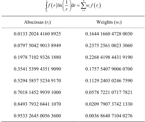
Owing to the subtraction technique, the singularity in the third integral on the right hand side of (45) as X ap- proaches _Y a _{is cancelled by the term in (46), and} similarly the seventh integral on the right hand side of (47) is also regularized. Even though the subtraction technique removes the strong singularity, the integrands in the first integral on the right hand side of (45) and the second integral on the right hand side of (47) still contain the weakly singular ln (r) term. The logarithmic singular- ity is integrable, but the accuracy of ordinary Legendre- Gauss integration is poor. We found that the special inte- gration scheme for the logarithmic singularity [22], which is reproduced in Table 1 for completeness, achieves ex- cellent numerical accuracy [1]. The remaining integrals of Equation (45) and Equation (47) are regular for which standard quadrature can be used with good accuracy.

In our numerical examples, the numbers of integration points were as follows: 8 integration points for any inte- gral along a straight line, and 8 × 8 integration points for any integral over a sub-domain. For regularized integrals, the usual Legendre-Gauss integration was used. For inte- grals containing logarithmic singularity, the special inte- gration of 8 integration points [32] as listed in Table 1

was used.

6. Enforcement of Boundary Conditions

[image:9.595.305.539.116.314.2]

Appropriate boundary conditions need to be enforced in order to solve the simultaneous Equations (44). In mesh-

Table 1. Special numerical integration for functions con- taining logarithmic singularity (8 integration points).

   

1

1 0

1

ln d N i i i

f r r w f r

r 

  _

 

 





Abscissas (ri) Weights (wi)

0.0133 2024 4160 8925 0.1644 1660 4728 0030

0.0797 5042 9013 8949 0.2375 2561 0023 3060

0.1978 7102 9326 1880 0.2268 4198 4431 9190

0.3541 5399 4351 9090 0.1757 5407 9006 0700

0.5294 5857 5234 9170 0.1129 2403 0246 7590

0.7018 1452 9939 1000 0.0578 7221 0717 7821

0.8493 7932 0441 1070 0.0209 7907 3742 1330

0.9533 2645 0056 3600 0.0036 8640 7104 0276

less methods, enforcing the essential (Dirichlet) bound- ary conditions is not as easy as in the finite element method. Because MLSA is non-interpolative, the essen- tial boundary condition cannot be accurately enforced by prescribing values for the fictitious nodal displacements (i.e., ˆa a

I I

u u ). A number of techniques for enforcing essential boundary conditions have been developed, in- cluding the collocation methods [33], Lagrange multi- plier method [34], penalty method [35,36], Nitsche’s method [37], coupled meshless-finite element method [38], and other methods [39-43]. The advantages and disadvantages of a variety of methods for enforcing es- sential boundary conditions have been discussed briefly in [1].

A number of collocation methods have been developed. The direct collocation method [33] used the condition

ˆa a I I

u u (48) to replace the row of the discretized weak form equation corresponding to the degree of freedom with prescribed displacement uIa . This is actually inconsistent with the assumption of MLSA since the fictitious nodal displace- ment ˆa

I

u is generally not equal to the approximated displacement value.

A generalizedcollocation method uses

 

1

ˆ n

a b a b a I I I

b

u  Y u u







 (49)

Generally, there are two types of discretization in meshless methods: 1) Galerkin based method over the global domain, which is used in EFG [33,42,47,48], clouds [41], RKPM [49-52]; and 2) localweakformover multiplelocaldomains, which is employed in [31,53-55]. For Galerkin based method over the global domain, the n system equations are obtained by applying the weak form over the global domain once, hence all equations must hold simultaneously in order to maintain consistency of the weak form. Replacing a row in the matrix equation by (49), which contains a linear combination of DOFs rather than dictating the single value of a constrained DOF, sacrifices the consistency of the weak form and compromises the solution accuracy.

For local weak form over multiple local domains, each equation is obtained by applying the weak form over a particular local domain, and the weak form needs to be applied n times for a problem with n DOFs. Conse- quently, the generalized collocation method with (49) can be directly used to enforce essential boundary condi- tions. Because each system equation is independent of the rest, replacing the equation corresponding to a con- strained DOF by (49) will not cause any inconsistency in the weak form.

As the current meshless integral method uses local weak form over multiple sub-domains, the generalized collocation method (49) is applicable. For a DOF with essential boundary condition, we simply use the condi- tion u_I u_I rather than applying the integral Equation (14). In numerical implementation, this means replacing the governing equation corresponding to the prescribed DOF with generalized collocation condition (49). Note that the governing Equation (14) holds for interior nodes as well as boundary (including corner) nodes, therefore Equation (49) is applied to nodes on smooth boundaries as well as at corners. Our numerical tests show that the generalized collocation method (49) for enforcing essen- tial boundary conditions works well for the meshless integral method.

For the natural boundary condition tI tI, no special treatment is needed. The prescribed traction is directly used in the second integral in Equation (47).

Although theoretically essential boundary conditions can be converted into the equivalent natural boundary conditions and the solution remains unchanged, we ob- served that the meshless method is always more accurate when essential boundary conditions are used.

After the boundary conditions are enforced, the gov-erning equations can be written as



,



1

ˆ y N

a b b a IJ J I b

K u R







(50)

where

 

 

, ,

, when is unconstrained

when

a b a b a b a IJ IJ IJ

a a b I IJ _{b a}

IJ

a a I I

H L

u K

u u

 

 

 _{ }

      

 _



Y

Y (51)

when is unconstrained when

a a a I I

I _{a a a} I I I

G u

R

u u u

  



 (52)

and the upper limit of summation, Ny, is the total num- ber of nodes in the domain of influence of node _Y a _. Detailed expressions of various terms are given in Equa- tions (45) to (47).

7. Solution Algorithm for Elastoplasticity

with Large Deformation

In this work, we will use the fixed point iteration to solve the governing equations which has the following advan- tages: the derivative of the stiffness matrix is not needed, and the implementation is relatively easy. With this algo- rithm, for each load increment, the stiffness matrix is computed only once in the first iteration.

The material considered in this study is rate inde- pendent, and therefore the actual loading rate has no ef- fect on the solution. It is, however, convenient to intro- duce a time parameter to describe the loading history. A piecewise linear function is used in the program to de- scribe the history of applied loads and is implemented in a table form in the input data. Each linear segment is referred to as a load step. For a loading history with N load steps, the corresponding data block takes the fol- lowing form:

0 0

1 1

2 2

, , ,

, N N

N

t P

t P

t P

t P

 

where n indicates the number of load steps. t t0, , ,1 tN are the times, while P P0, , ,1 PN are the corresponding load levels. Both t0 and P0 are set to zero if the initial

state is load free.

Since the elastoplastic integral equations are strongly nonlinear, loads have to be applied in small increments, and iterations are needed to achieve convergence within each load increment. For the first load step P1 at a level

load from rP1 to



1r P



1 is then divided into M in-

crements. Within each load increment, the solution is iterated until convergence. For subsequent load steps, the load is incremented in a similar manner.

Throughout this section, we use

 

var _{ } _mi to denote a variable

 

var (which may be displacement, stress or strain) for m-th load increment at i-th iteration, and use

 

var _{ m} to denote the converged solution for m-th load increment.

7.1. Solution Algorithm

1) Divide the load into N load steps, set the load in- crement number M for each load step and maximum it- eration number Imax; initialize the load step index n, load increment index m, and iteration index i to 1.

2) For load step index n and load increment index m, the convergent state at (m – 1)-th load increment will be used as the reference configuration. Set the initial dis- placement relative to the reference configuration

 

_{ }0

 

0

m

U  , and compute the stiffness matrix [K] based on the reference configuration. Set the second Piola- Kirchhoff stress

 

T  0 

 

 , where

 

 is the con- vergent Cauchy stress at (m – 1)-th load increment.

3) For iteration index i, use Equations (53)-(55) to up-date the solutions.

 

_{ } 

 

    

 

  

1 1 1

i i m i

m m m

F  K U  LDEP U  (53)

 

 

 

   

  

1 i i

m

K U   R F  (54)

 

_{ } 

 

  

 

 

1

i i i m m

U  U   U (55) where

 

ΔR is the load increment from (m – 1)-th load increment to m-th load increment. LDEP U

 

_{ } _mi1 are the nonlinear terms because of large deformation and elastoplasticity corresponding to the third to sixth terms of the Equation (47) for m-th load increment at (i – 1)-th iteration.

4) The following convergence criterion is used to ter-minate the iteration for each load step:

   

_  _

 

1 ₂ 2

i

f m

R F _  R

    (56)

f

 is a predefined tolerance, usually in the order of

4 7

10 ~ 10  _.

a) If the program converges in this iteration, update the geometry, the displacement field, and the second Piola- Kirchhoff stress for each Gaussian point (Section 7.2) and obtain the corresponding Cauchy stress by Equation (57):







0







, ,

IJ IK uI K TKL TKL JL uJ L J

          (57)

where J is the determinant of the deformation gradient F

which is defined as follows:

x x

X Y

y y

X Y

 

 

_{ } 

  

 

 

_{ } 

 

F (58)

then go to step 5.

b) Otherwise, increase the iteration index by one and check if i is greater than Imax. If yes, the program cannot converge for the preset Imax, exit program execution; otherwise, compute the second Piola-Kirchhoff stresses at all Gaussian points for all nodes and go to step 3.

5) Increase the load increment index m by one and check if m is greater than load increment number M. If yes, exit the program; otherwise, go to step 2. The inte- grals for next load increment are to be performed over the deformed geometry of converged solution of current load increment, and the converged current configuration will be the reference configuration for the next load in- crement, hence the updated Lagrangian formulation.

As shown in the previous section, the nonlinear terms

 

_{ } i1 m

LDEP U  (the third to sixth terms of the Equation (47)) for m-th load increment at (i – 1)-th iteration are needed in order to calculate the internal force

 

F _{ } _mi1. The integration is usually performed using Gaussian nu- merical integration. Therefore, the stress state, along with the stress correction term, is computed at all Gaussian points in each iteration step. The following section de- scribes the algorithm to compute the stress at each Gaus- sian point.

7.2. Procedure for Computing Stresses at Each Gaussian Point

1) After the solution is converged for (m – 1)-th load increment, the corresponding Cauchy stress using the second Piola-Kirchhoff stresses which are basic stress measure obtained from solution is computed. The Cauchy stress obtained is then used as the initial value of the second Piola-Kirchhoff stress

 

T _{ } 0_m for the m-th load increment. Given

   

 u U _ _mi_1

 

U _{ m} , the strain increment

 

E and the stress increment

 

_Te _are initially predicted assuming elastic behavior using (59) and (60) shown below.

 

 and

 

_Te _{, needed to} compute the fourth term of Equation (47), are predicted by Equations (61) and (62) with

 

cor _{ }

m

T and

 

e _{ } m

T



, , , ,



1 2

IJ I J J I K I K J

E u u u u

        (59)

 

_Te _{ C}e

 

_E

  (60)



, ,



1 2

IJ uI J uJ I



     (61)

 

_Te _{ C}e

 

_

  (62)

2) Determine the loading state

2.1) If EPF = 1, the Gaussian point is in an elastoplas- tic state in previous load step. Compute the loading crite- rion function L using Equation (18). Use parameter r to denote the scaling factor such that

 

_{ }

 

_{ }



e ,



0

m m

f T  r T   (63)

If L > 0, let r = 0, plastic loading occurs; if L≤ 0, let r = 1, EPF = 0, compute the yield function after the trial stress increment is applied

 

_{ }

 

_{ }



e ,



m m

f T  T 

if f 0, let r = 1 and EPF = 0, the point remains in the elastic state; if f 0, let EPF = 1, the point enters into elastoplastic state, determine scaling factor r using (63). Update the stress at this point by

   

_{ }

 

e

m

T  T  r T (64)

2.2) If EPF = 0, the Gaussian point is in an elastic state in the previous load step. Compute the yield func-tion after the trial stress increment is applied

 

_{ }

 

_{ }



e ,



m m

f T  T 

if f 0, let r = 1 and EPF = 0, the point remains in the elastic state; if f 0, let EPF = 1, the point enters into elastoplastic state. Determine scaling factor r using (63). Update the stress at this Gaussian point using Equation (64).

3) Compute the sub-increment of strain

 

E :

 

(1 r)

 

E E

N

 

  ₍₆₅₎

where N is an integer. Integrate numerically to compute sub-increment of stress

 

Tij with n looping from 1 to

N.

 

T  n is used to denote the second Piola-Kirchhoff stress increment at the end of n-th iteration and let

 

 0





0 cor

T T

    :







2

2

9 2

3 1

2

kl kk ij

ij ij kk ij

p e

IK JL JK IL IL JK JL IK

IJ KL KL

T E T

T E E

H

E



  

 

       

 

      

 

 _   

 

  



(66)

 

 n

 

n1

 

T T  T

     ₍₆₇₎

4) Update the variables:



_Tcor



_{ }

 

_T  N _{ r}

   

_Te _{ T}e ₍₆₈₎

 

_{ } 

 

 





i

cor cor cor m m

T  T  T (69)

 

_{ } 

 

 

 

 

 

0

i N e m m

T  T  T  r T (70)

 

_{ } 

 

 

 

i

e e e m m

T  T  T (71)

7.3. The Computation of Nonlinear Terms For the third term in Equation (47), ,



,



a IJ K

u X Y

needs to be computed, which is the derivative of



, a



IJ

u_ _{X Y with respect to} K

X . Equation (69) is used to calculate

 

_Tcor _{for each Gaussian point, and the} third term in Equation (47) is computed accordingly. Equation (71) is then used to calculate

 

_Te _{which is}

equal to ,

e

LKMN M N

C U and the fourth term of Equation (47) is computed accordingly.

As for the fifth and sixth terms of Equation (47), 0 LK

T is the initial value of the second Piola-Kirchhoff stress of