J. Range Manage.
48:73-80 January 1995
How much sagebrush is too much: An economic threshold analysis
CHRIS T. BASTIAN, JAMES J. JACOBS AND MICHAEL A. SMITH
Authors are assistant extension educator and professor, Agricultural Economics Departmeni and professor, Range Management Department, respectively, University of Wyoming, Luramie, Wyo. S2071.
Abstract
Much research concerning sagebrush control methods and for- age response after control has been conducted due to the impor- tance of sagebrush-grass dominated rangelands for livestock and wildlife in the western United States. Very little research has addressed the economic feasibility of sagebrush control at vari- ous levels of abundance. This study estimates the economic threshold abundance of sagebrush based on forage response data from a sagebrush control experiment in Carbon County, Wyo.
Forage response data are based on the difference in herbage between treated and untreated experimental units from sites ranging in initial sagebrush canopy cover from 4 to 40%.
Breakeven returns per AUM were estimated for each sagebrush canopy cover level assuming 2,4-D (2,4-dichlorophenoxyacetic acid) or burning (for 28 to 40% canopy cover) as a control method with lives of control at 15, 20, and 25 years. These breakeven returns were compared to a net lease rate of
$6.13/AUM. Results indicate the economic threshold abundance of sagebrush is 12% assuming, 2,4-D as the control method and a control longevity of 25 years, but the feasible sagebrush abun- dance increases as longevity of control decreases. If the longevity of the control only lasts 20 years, the sagebrush abundance must be at least 20% before treating sagebrush becomes economically feasible. If the longevity of control is only 15 years, sagebrush abundance must be at least 24% canopy cover before treatment is economically viable. Given estimates of the cost of burning are almost half that of spraying with 2,4-D, all the scenarios which had enough biomass to sustain a bum (28% to 40%) indicated sagebrush control by fire was economically viable.
Key Words: Artemisia tridentata ssp. ~yomingensis, breakeven return per AUM, lie of control, 2,4-D, and burning.
The sagebrush-grass ecosystem occupies a substantial portion of rangelands in the western United States. Acreage estimates of sagebrush-grass rangeland vary from 30 million ha to 109 million ha (Blaisdell et al. 1982). Estimates indicate that big sagebrush (Artemisia tridentata Nutt.) is the dominant range cover on approximately 39 million ha in the West (Alley 1965). Since sagebrush-grass rangelands are used predominantly to produce
hianuscript accepted 28 May 1994.
forage for livestock and wildlife, sagebrush control methods, degree of control and forage response have been the subject of much research.
Research has primarily focused on control methods and forage response after control. The literature indicates burning and spray- ing with 24,D are the most successful and cost effective methods for controlling sagebrush (Kearl and Brannan 1967, Kearl 1965, Krenz 1962, Mueggler and Blaisdell 1958, Smith et al. 19S5).
Forage response after control varies greatly, from 0 to 400% of production on comparable uncontrolled sites, depending on such factors as precipitation, composition of understory vegetation, sagebrush mortality, method of control, grazing management after control, and density of sagebrush population before control (Alley and Bohmont 1958, Bartolome and Heady 1978, EPA 1972, Kearl and Brannan 1967, Kearl 1965, Mueggler and Blaisdell 1958, Pechanec et al. 1954, Smith and Busby 19S1, Sturges 1986, Tabler 1959, Tanaka and Workman 198X, Wambolt and Payne 19S6).
Information concerning control methods and forage response is important to the range manager when making sagebrush control decisions. A major problem for managers is identifying a site where (1) the infestation of sagebrush is dense enough to cause a significant reduction in forage yield and (2) the potential increase in forage production would be sufficient to economically justify the control of sagebrush (Jacobs 1987).
Early research focused on the question of proper chemical mis- hue and recommended percent sagebrush mortality rather than identifying economic threshold sagebrush densities. Hull et al.
(1952) treated plots of sagebrush averaging 25 to 30 plants per 30.5 rrr’. They used a total of 57 different herbicide and carrier mixtures in 1949 and 59 different mixtures in 1950. They con- cluded grass production could be increased 2 to 3 times in 2 years after chemical control of sagebrush as long as there was fair grass understory before treatment. They also concluded the increases were to some degree proportional to the percent of sagebrush plants killed. Native grass production was increased approsimate- ly 2 to 3 times by killing 60 to 97% of the sagebrush.
Alley (1956) used different rates and esters of 24-D and 2,4.5-
T to better understand chemical control of sagebrush and the cor-
responding forage response after control in the Bighorn
Mountains of Wyoming. Sagebrush clumps “averaged 26.9 inch-
es in height by 30.0 inches in diameter and 32 clumps per square
rod” (Alley, 1956). By sampling vegetation within the treated and
untreated strips Alley (1956) determined the influence of various
degrees of sagebrush control upon the grass-like species, forbs and shrubs. Data was summarized on the basis of 0,50 to 7576 to 95, and 96 to 100% of sagebrush control. Alley (1956) con- cluded native grass production was increased as control of sage- brush increased. The most grass production was observed in the 96 to 100% sagebrush controlled areas.
Miller et al. (1980) tried to document changes in forage produc- tion and plant species abundance following application of 2,4-D in three mountain big sagebrush (Artemisia tridentata ssp.
vaseyana (Rydb.) Beetle) habitat types. Shrub cover varied behveen 21 and 33% canopy cover on the 3 habitat types. Percent mortality of sagebrush ranged between 81 and 97%. Across the three habitat types bluebunch wheatgrass (Agropyron spicatum (Pursh) Scribn. and Sm.) was more responsive on the sprayed sites than Idaho fescue (Festuca idahoensis Elmer). Total forb production was lower on sprayed sites.
Whitson and Alley (1982) established experimental plots near Ten Sleep, Wyoming on sagebrush infested land to evaluate the potential of tebuthiuron (N-[5-( I,1 -demethylethyl)-1,3,4-thiadia- zol-2-yl] -N,N’-demethylurea} as a potential chemical control method on sagebrush. Three rates of 20% granular material, 0.29, 0.62, 0.86 kg/ha a.i. (active ingredient), were applied. Oven dry yields gathered 3 years after control from the 0, 0.29, 0.62, and 0.86 kg/ha rates were 283, 35 1,658, and 508 kg/ha, respectively.
Sagebrush defoliation for the 0.29,0.62, and 0.86 rates of tebuthi- uron were 69,96, and 99.5%, respectively.
Clary et al. (1985) studied the effectiveness of tebuthiuron in controlling woody plants on Utah juniper (Juniperus osteosperma (Tom) Little) and mountain big sagebrush dominated sites and evaluated responses of herbaceous species. Application rates of 0, 0.6, 1.0, and 1.3 kg/ha a.i. of 10% pellets was applied on the mountain big sagebrush strips. The authors found a high propor- tion of control at the 0.6 (approx. 80%) rate and nearly complete control of the original sagebrush plants at the 1.3 kg/ha rate (approx. 93%). Total production of herbage (including leaf and twig growth on shrubs) (-0.05) was not significantly different from the control in the third growing season after sagebrush treat- ment. Fairway wheatgrass (Agropyron cristatum (L.) Gaertn.) was initially depressed, but recovered by the third year.
Hull and Klomp (1974) tried to evaluate 3 different control methods at different big sagebrush densities and how that affect- ed, (1) yields of crested wheatgrass (Agropyron desertorum (Fisch. es Link) Schult) growing under sagebrush, (2) amount of rain and snow reaching the soil and (3) soil moisture content. In 1950 and 1954 several sites in Idaho were cleared of sagebrush and seeded to crested wheatgrass. Big sagebrush reinvaded seed- ed ranges to a density of 20 plants per 30.5 meters’. In 1965 big sagebrush was reduced to 10,5, and 0 plants per 30.5 meters? (50, 75, and 100% kills) by grubbing, burning, and spraying with 2,4- D. The authors concluded that the 3 methods of control did not differ in the amount of grass produced following brush control, and where wildlife or livestock do not need sagebrush, all the brush should be killed. Any remaining sagebrush suppresses grass and produces seed for reinvasion.
Tanaka and Workman (1988) extended Hull and Klomp’s (1974) work into an economic framework developed for estimat- ing the optimum rate of initial overstory kill for increasing sea- sonal forage availability. The model was formulated using, (1) biological data from Hull and Klomp (1974) to estimate a pro- duction function relating understory production to initial kill per- centage, (2) a derived demand function for seasonal forage value
by using linear programming to estimate shadow prices for addi- tional production of crested wheatgrass, and (3) a cost of oversto- ry kill function for each control method. Tanaka and Workman (1988) used the big sagebrush- crested wheatgrass vegetation type on a “typical case ranch” (cow-calf-yearling operation) in Utah. For the case ranch analyzed, a big sagebrush kill rate between 92 and 100% was optimal.
While these pieces of research tried to ascertain forage respons- es using different chemical mixtures, in different habitat types and different percentages of sagebrush mortality, they do not pro- vide much information in terms of what initial sagebrush abun- dance level will be economically feasible to consider control.
Additionally, today’s managers must consider the possible envi- ronmental effects sagebrush control might have on ecosystems managed for multiple uses. These economic and environmental factors preclude a manager from indiscriminately controlling sagebrush. Managers need additional information to aid them in assessing whether sagebrush control is an economically viable alternative.
The focus of this study is to determine the economic threshold abundance level for big sagebrush control. The economic analysis in this study is based on forage response data from a study of sagebrush control in Carbon County, Wyo.
Materials and Methods Study Area
The forage response data comes from an area in southcentral Wyoming, approximately 19 km northeast of Saratoga, Carbon County, Wyo. The area is on the west slope of the Medicine Bow mountain range at an elevation of 2,245 m and receives about 33 cm of precipitation annually. Vegetation in the area is dominated by an overstory of Wyoming big sagebrush (Artemisia tridentata ssp. wyomirzgensis Beetle and Young) with an herbaceous layer featuring western wheatgrass (Agropyron smithii Rydb.) and nee- dle-and-thread grass (Stipa comata Trin. & Rupr.). Forbs are not abundant in the study site.
Within this area, 20 study sites were selected across a range of big sagebrush abundances as measured by canopy cover, but on similar sandy soils and topographic positioning. On each study site 2 experimental units (approximately 30 m by 30 m each) with the same big sagebrush abundances were selected and randomly designated, one with sagebrush controlled and the other not treat- ed. Two replicate pairs of each sagebrush abundance level were included in the design. Sites had big sagebrush canopy cover (cover was determined using 6-100 point transects) ranging from 4 to 40% in approximately equal increments.
Big sagebrush was treated by spraying with 24-D in early June of 19S7’. For each study site, peak standing biomass of all herba- ceous vegetation has been measured in late July each year of the study by harvesting vegetation on quadrats protected by movable cages (6 per experimental unit). The herbaceous biomass consist- ed primarily (approx. 90%) of western wheatgrass and needle- and-thread grass. A small portion of the clipped herbage some- times included annuals and forbs (approx. 10%). All of the herbage was usable by cattle and sheep at least during part of the
‘It is important to note that ground application of 2.4-D occurred in June 1987 on the study sites in Carbon County, Wyo. for the experiment used in this analysis.
Sagebrush control was in excess of 95% mortality on all treated sites.
74 JOURNAL OF RANGE MANAGEMENT 48(l), January 1995
grazing season. The difference in herbaceous biomass between the treated and untreated experimental units was assumed to be the forage response due to controlling sagebrush.
Table 1. Forage Response (difference between controlled and uncon- trolled sites) adjusted for differences between sites in seasonal precipi- tation and soil moisture (Dhl basis).
These data were adjusted for precipitation and soil moisture differences among study sites using regression analysis. While these models are linear in nature, it is important to remember that they are used to normalize the data, and they are not a simulation or production function model used to estimate production over the life of the sagebrush control. Assumptions concerning the pat- tern of utilization over the life of control will be discussed later in the economic analysis section of the text.
% Saeebrush Canow Cover
Year 4% 8% 12% 16% 205 24% 28% 32% 36% 40%
1987’ Kg/ha
1988 17 50 83 116 150 183 216 249 282 315 19X9 124 157 190 223 256 289 322 356 389 422 1990 230 263 291 330 363 396 529 462 495 528 1991 337 310 403 436 469 502 536 569 602 635
‘Year of ueamenr Grazing considered to be deferred and forage not utilized.
Linear regression models used to normalize the data should be fairly accurate across the sites. Sala et al. (1988) found produc- tion at the site level was largely accounted for by annual precipi- tation, soil water-holding capacity, and an interaction term. This simple linear model accounted for 90% of the variation in pro- duction from site to site. Sala et al. (1988) found the addition of other climatic variables such as potential evapotranspiration, tem- perature, or the precipitation:potential evapotranspiration ratio for the growing season or the entire year did not significantly improve the model. The more sophisticated models including such variables did not account for more than 90% of the variation in production.
The variables used to estimate the regression parameters for calculating the adjusted production data across experimental sagebrush sites for this study were percent sagebrush (sage), pre- cipitation for April, May, and June (precip), percent May soil moisture for check plots (mayc), percent soil moisture for treated plots (mayt) and year (yr). The regression models were as fol- lows:
tion was assumed to be a function of treating the sagebrush.
These regression adjusted differences are reported in Table 1.
Economic Analysis
Information needed to identify the economic threshold abun- dance level of big sagebrush includes the control methods to be analyzed and their associated costs, quantification of herbage responses and utilization associated with treatment, and valuation of the forage over the life of control.
Control Methods and Associated Costs
MODEL FOR UNTREATED CHECK PLOTS Yield= 8, + 13, sage + B2 precip + 13s Mayc + 0, yr + &
MODEL FOR TREATED PLOTS
Yield= B, + 13, sage +- D2 precip + l3, Mayt + RG yr + &
where:
B’S = estimated regression parameters
Yield = Yield based on clip data for that year and corresponding plot
sage = percent sagebrush (4 to 40)
precip = sum of precipitation collected from site gauges April, May and June for each year of study period
Mayc = soil moisture for each year of study period in May on check plots
Mayt = soil moisture for each year of study period in May on treated plots
yr= Year (1987= -2,19SS= -1,1989= 0,1990= 1,1991= 2)
&= Error
The normalized yields were estimated by calculating the pre- dicted yields for each year and percent sagebrush using the esti- mated regression parameters, mean soil moisture for the study period for both the check plots and the treated plots and mean precipitation for the months of April, May, and June during the study period. These normalized yields were designed to take out variability associated with differences in annual precipitation from year to year and differences in soil moisture across study sites, so that yield differences for each year were associated with percent of sagebrush. The differences in these normalized yields between treated and untreated plots for each level of sagebrush abundance was then estimated and the increased forage produc-
Several techniques are available for sagebrush control. Much of the earlier research looked at chemical control with 2,4-D.
However, other methods of chemical control, as well as, burning and mechanical control are available to the land manager. Each one of these alternatives needs to be evaluated by the individual manager in terms of characteristics of the land, managerial objec- tives for the operation and economic feasibility.
Tebuthiuron has been found to control big sagebrush at the application rate of 0.6 to 1.1 kg a.i./ha by Whitson and Alley (1984). However, several drawbacks may exist with the use of tebuthiuron. Steinret and Stritzke (1977) found that phytotoxicity decreased forage production the first year after tebuthiuron appli- cation. Britton and Sneva (1983) found that mean herbaceous yields decreased with each increased rate of tebuthiuron.
Bjerregaard et al. (1977) found forage yields were depressed for two years after application, but production increased later and the residual tebuthiuron showed potential for effective control against sagebrush seedlings for several years. Whitson and Alley (1984) observed that in the first year following application of tebuthi- uron cool season grasses were chlorotic in appearance. However, reduced symptoms were noted in subsequent years.
Burning is an effective method for controlling sagebrush (Smith and Busby 1981). Mueggler and Blaisdell (1958) con- clude that burning is by far the least espensive sagebrush control method despite the 1 year grazing deferment. Wambolt and Payne (1986) concluded that of 4 control methods, burning,
spraying with 2,4-D, rotocutting and plowing with seeding, bum- ing was most effective in reducing sagebrush canopy. Plowing with seeding was found to be least effective. After 18 years bum- ing provided the most production from dominant forage species and important vegetal classes, but burning and spraying were equally successful when production was totaled for all years sam- pled.
Shariff (1988) studied vegetation, soil moisture, and nitrogen
responses with respect to 3 different methods used in controlling
big sagebrush. This study compared 2,4-D, burning and tebuthi- uron. Shariff concluded that the bum treatment exhibited the best response in the control of big sagebrush and total production. The 2.4-D treatment was found to be as effective as the bum treat- ment when the proper timing and application techniques were used. These conclusions concerning burning and spraying with 2.4-D are consistent with Hull and Klomp (1974). The tebuthi- uron treatment appeared to be effective only on loamy soils.
In this study, spraying with 2,4-D was the method of control used on the experimental units. For this analysis $26.54/ha2 is used as the chemical and application cost for 2,4-D. Given the findings of previous studies, this analysis also explores burning as a control method. According to data from the Soil Conservation Service average cost of burning in several Wyoming counties was estimated and adjusted for inflation to represent 1987 dollars. The estimated cost of burning used in this analysis was $13.73/ha3.
The burning scenario is only estimated for those experimental units which had enough biomass to sustain a bum. Smith et al.
(1985) found when brush cover is below 30%, fine fuel amounts must exceed approximately 333 kg/ha (for continuous sod form- ing species) to near 667 kg/ha (for discontinuous bunchgrass or rhizomatous wheatgrass species) for good fire spread to occur. If brush cover exceeds 30-35%, fire spread will usually occur with lesser amounts of fine fuels. Given these criteria, those plots exhibiting 28 to 40% sagebrush cover were considered feasible for the bum scenario in this analysis.
One year of grazing deferment after treatment is assumed in this analysis. This is an additional cost associated with treatment which must be recaptured over the life of the control. An oppor- tunity cost of not grazing that first year after treatment is calculat- ed and added to the cost of treatment. The normalized yield data on the untreated plots for 1987 is multiplied by a 50% utilization rate and a conversion factor of 360 kg DM/AUM (Society for Range Management 1974, Scamecchia and Kothmann 1982) to estimate animal unit months (ALJM) of grazing forgone for each level of sagebrush abundance. The AUM’s of grazing forgone is then multiplied by a net forage value of $6.13/AUM to estimate the opportunity cost of deferment in the first year of treatment.
The net lease rate of $6.13/AUM is an average of common lease rates for Wyoming during the years of 1981 to 1991 minus an estimate of 30% of the lease rate associated with services provid- ed by lessors and adjusted to 1987 dollars (Wyoming Agricultural Statistics Service 1993, Torrell et al. 1988).
Quantification of Herbage Response and Utilization
Increased forage production resulting from sagebrush control lasts for varying periods. The longevity of control and amount of increased forage production varies from site to site and is influ- enced by degree of control. Johnson and Payne (1968) found that unkilled sagebrush was the major cause of reinvasion. Hull and Klomp (1974) found that killing the last 25% of a big sagebrush stand resulted in 98 to 135% more crested wheatgrass than hilling the first 75% at southern Idaho sites.
In order to evaluate the feasibility of sagebrush control, the quantification of increased forage production must be estimated throughout the life of control for relevant planning horizons.
This based on commercial rates from Sky Aviation in Worland, Wyo. for 1957.
This is based on personal phone interviews wth personnel in the Cheyenne and Buffalo offices.
Kearl and Brannan (1967) used different figures for effective life of control depending on observed results for different methods.
Chemical spraying with 2,4-D had a projected life of 15 years.
Kearl and Freebum (1983) found sites sprayed on National Forest land to be highly productive after 20 years. Tanaka and Workman (1988) used a planning horizon of 25 years for sagebrush control.
Based on the literature and the sagebrush mortality on the experi- mental sites, 15 to 25 years is used as a reasonable planning hori- zon for the economic threshold analysis.
It is also important to understand long term trends in forage response, as well as utilization of forage to quantify the value of herbage response after sagebrush control. Blaisdell et al. (1982) discussed trends in sagebrush reinvasion and grass production after a controlled burn near Dubois, Ida. from 1936 to 1966.
Much of the discussion was based on Hamiss and Murray (1973).
Over the 30 year period, mountain big sagebrush demonstrated a very dominant role in the plant community. During the first 12 years following burning, nearly all species of grasses, forbs and other shrubs increased in yield. In the subsequent 18 years fol- lowing the burn, yields of the grasses, forbs and other shrubs decreased as sagebrush regained control. Forage production returned close to the prebum levels by the end of the 30 year peri- od.
The economic analysis by Kearl and Freebum (1983) assumed the usable forage production doubling in 2 years, forage produc- tion being sustained for years 3 through 10 and then forage pro- duction declining to the pretreatment levels in years 11 through 15. Jacobs (1987) used forage utilization by livestock to depict an increase in physical response due to sagebrush control. Jacobs assumed forage utilization to increase by 50% in year 2, 100% in year 3, sustained levels of utilization equal to year 3 in years 4 through 10 and forage utilization declining to pretreatment levels in years 11 through 15.
Tanaka and Workman (1988) however, based the production function on the assumption that any increase in forage from an overstory treatment remained constant from the first year of graz- ing until the end of the project life. The production function val- ues were adjusted for both desired utilization rate and availability of forage to livestock. The availability function was based on observations by Hull and Klomp (1974) and assumed to be linear between 40 and 90% as big sagebrush canopy varied from 34 to 0%.
Workman and Tanaka (1991) illustrate several cases which suggest as utilization of forage increases and or sagebrush mortal- ity decreases, reinvasion of sagebrush increases. In the first dynamic case illustrated by Workman and Tanaka (1991) a 50%
utilization rate and 95% initial overstory removal is assumed.
This case resulted in a 20 year project life due to big sagebrush encroachment, while a 75% utilization rate and 95% mortality on sagebrush resulted in a 15 year project life. In the case where only 50% of the sagebrush were removed and 50% of the forage was utilized the projected life was 10 years.
Unfortunately, for this analysis only 4 years of forage response data is available for analysis (Table 1). Based on Blaisdell et al.
(1982) and Hamiss and Murray (1973) it seems reasonable to expect the forage response after sagebrush control to increase over a period of years and then decrease as sagebrush reinvades the treated area. It also seems reasonable based on the previous discussion to expect sagebrush control to last between 15 and 25 years. For this analysis, assumptions concerning the utilization of the forage are used to take into account a forage response curve.
76 JOURNAL OF RANGE MANAGEMENT48(1), January 1995
Increased forage utilization is based on the adjusted production data in Table 1. One year of grazing deferment is assumed. It is also assumed that only 50% of the increased forage production is utilized annually and that 360 kg DM provides 1 AUM.
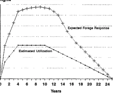
h,Ia..imum forage utilization increase is assumed to occur in year 4. It is further assumed that this level of utilization is maintained until year 10. The increased forage utilization is assumed to decrease in equal increments after year 10 as sagebrush reinvades until the infestation reaches the pre-treatment level at the end of the specified planning horizon. Figure 1 illustrates the expected forage response versus the estimated forage utilization over the life of the control.
Valuation of the Forage and Estimate of Breakeven Price Over the Life of Control
Range managers may have different objectives for controlling sagebrush, and thus, different values may be placed on the increased forage production associated with treatment. Due to the unique characteristics of each individual situation, different val- ues may need to be considered by a range manager. Workman ( 19S6) discusses several possible approaches. One approach is to use a private lease rate. This “market value” approach is deemed reasonable because a manager would have an opportunity to lease these AUMs to stockmen if returns to the operation from the additional forage were less than the lease rate. Nielsen and Hinckley (1975) and Stevens and Godfrey (1976) used lease rate approaches to value additional forage from range improvements.
Workman and Tanaka (1991) state that in many cases valuing revegetation benefits as privately leased forage is simple, straightforward and often yields accurate estimates of the value of additional forage particularly when the operation currently leases and or can avoid leasing forage in the future due to the improve- ment.
Private range lease rates, however, do have some caveats asso- ciated with valuing forage for an improvement. Jacobs (1987)
Kg/ha
. . . . . . . .._ . . . ..I . . . ..*...
. . . . . . .A+,. . ..-.. . .
I/ -f- . . . . . . .._.. . . . “k . . . ...
0 2 4 6 8 10 12 14 16 18 20 22 24
Years
Fig. 1. Illustration of expected forage response curve versus estimat- ed utilization based on assumptions used in the analysis.
states that while some economists feel that grazing lease rates are a defendable value, they may tend to overestimate the value of forage for several reasons. One problem is lease rates may include a number of services as a premium (for example lessor may provide salt, fence repair, and herding). Workman and Tanaka (1991) report that published private lease rates include a premium for landlord services of about 30% (Tore11 et al. 1988) and that the value of additional forage, itself, is only about 70%
of published lease rates. A second problem according to Jacobs (1987) is that most grazing fees are based on short term leases. In many instances a producer would only consider variable costs when determining the maximum lease rate that would be feasible.
Due to the short run nature of a lease “market value” of the for- age could be higher than a long term arrangement where the fised and variable costs are both considered. Workman and Tanaka (1991) note that pricing at the private lease rate often yields a higher revegetation benefit than does valuation as increased live- stock production (Workman 1986).
Due to the possible shortcomings of grazing fees some econo- mists prefer a total ranch budgeting approach when valuing addi- tional forage from a range improvement. Nielsen (1967), Kearl and Freeburn (1983), and Tanaka and Workman (1988) all took a ranch budgeting approach. The general technique was to estimate additional ranch income due to the improvement. These addition- al income flows were then discounted back to present value and compared to the cost of the improvement. For a producer, a bud- geting approach based on the specific requirements of the indi- vidual operation could offer more accurate information concem- ing the added profitability from a proposed improvement.
According to Workman (1986) ranch budgeting might also be used to calculate the average value of an added AUM. All non- forage costs can be subtracted from annual gross ranch income.
The result of that calculation could then be divided by the total number of AUMs of forage used by the operation annually. This average value might then be used to do the analysis.
Perhaps the biggest advantage to a total ranch budget approach is this approach requires the manager to inventory all the resources available to the operation and decide whether the improvement can be done without creating a shortage elsewhere (Nielsen 1967). The producer may not want to increase spring grazing if the operation cannot meet the increased hay require- ments brought on by increased stocking due to the improvement for example.
Unfortunately, the ranch budgeting approach is more compli- cated in terms of accounting for all resource inventories, valuing and planning the timing of resource usage and accurately reflect- ing all the effects of the improvement. Workman (1986) suggests the complexity of this approach is the biggest drawback. The ranch budgeting approach has some shortcomings for a researcher trying to make general recommendations concerning various improvements. The “typical case ranch” budget may be less representative of the intended audience of the research than a market value or lease rate approach. For this study, a large num- ber of scenarios are investigated concerning initial sagebrush canopy cover levels, control methods and associated costs and different planning horizons for longevity of control, and the results are intended for a relatively broad audience of managers who might consider sagebrush control as an alternative. Thus, the ranch budgeting approach seems less desirable.
This economic analysis estimates the breakeven price the
increased forage production must receive per AUM for each plan- ning horizon, method of treatment and sagebrush abundance level to cover the initial cost of control and opportunity cost of defer- ment. The higher the breakeven price the less likely the range improvement will be feasible given the manager’s objectives.
Since the investment in sagebrush treatment is not recaptured immediately, the returns associated with control must be dis- counted over the life of the control. Nearly all individuals display a positive time preference for money (Barry et al. 1983). A dollar received today is preferred to a dollar received a year from now.
Thus, for an investment to be economically feasible, the sum of the future returns from the investment discounted to a present value must be greater than or equal to the initial cost of the investment.
The net present value (NPV) method uses discounting formulas to obtain the value of the projected cash flows associated with an investment alternative. In this fashion, the net present-value crite- rion directly accounts for the timing and magnitude of the pro- jected cash flows for alternative investments having different
planning horizons and cash flows. Given the concepts used in the net present value method, the following formula was derived and used to estimate the breakeven prices (PF in formula) for this analysis. The PF (price of forage) value was solved for in an iter- ative fashion until NPV was equal to zero or as close to zero as possible without being negative.
TRTCST = ; UIJFI * (PF,) n n=O (1 +ip
Where:
TRTCST = Cost of treatment (including deferment).
UF = Increase in utilizable forage due to treatment (converted to ALMS).
i = Discount rate.
N = Number of years in planning horizon.
PF = Price of forage per AUM.
(WWPF))n = The return received for each conversion period (n) due to controlling sagebrush.
To express the value of the income flows in present terms they must be discounted at a relevant rate (i in the above equation).
Barry et al. (1983) state that for capital budgeting procedures the discount mte is a firm’s required rate of return on its equity capi- tal. The discount rate is generally considered to contain 3 compo- nents. There is a risk free rate for time preference, a rate reflect- ing the riskiness of the expected net cash flows and an inflation premium. The authors go on to state that the discount rate is much like an opportunity cost and should reflect a rate the firm’s equity capital could earn in the most favorable alternative use.
Workman (1986) discusses criteria for picking a discount rate which are consistent with Barry et al. (1983). He states that ideal- ly a discount rate should be the higher of either the interest rate on borrowed capital for the improvement or the opportunity cost rate. Given the best alternative use of range improvement capital is not always known, Workman (1986) suggests a representative borrowing rate is often used for discounting or comparison pur- poses. Generally since returns are measured in real terms, the appropriate discount rate should be in real terms as well.
For this analysis a discount rate of 6% was chosen. This was based on a long term (1950 to 1992) average real prime interest rate of 3% (U.S. Government Printing Office 1993) plus a 3%
risk premium. Tanaka and Workman (1988) used a 7% discount rate, using a 4% rate plus a 3% risk premium. The higher the dis-
count rate the larger breakeven price of the forage would have to be over the life of control to cover the initial cost of control plus the opportunity cost of deferment. For example, if the maximum increase in forage utilization was based on an increase of 232 kg/ha in year 4 using 24-D and with a 20 year expected longevi- ty, the average value of the increased forage or breakeven price would have to be $11.08/AUM to cover the cost of treatment at a 6% discount rate. At a 7% discount rate, assuming everything else remained the same, the price of the forage would have to be
$11.92/AUM, and if a 10% discount rate were used, the breakeven return for the forage would increase to $14.82/AUM.
These estimated breakeven forage prices (PF) must be com- pared to estimates of what that forage is actually worth before conclusions can be drawn about which initial sagebrush abun- dance level could be considered as economically feasible to con- trol. As mentioned earlier, one problem with private grazing leas- es is the lease rate may include a number of services (for exam- ple, salting, fence repair, and herding). Thus, a net lease rate which has these types of services subtracted out may more accu- rately reflect the value of forage. A net lease rate of $6.13/AUM is used as an estimate for comparison in this analysis.
Conclusions concerning the economic threshold level of big sage- brush are drawn by comparing this inflation adjusted value less services to the estimated breakeven prices for each scenario.
Results
A breakeven return per AUM has been calculated for each sagebrush abundance level, life of control and treatment method scenario (2,4-D, bum) with only half of the increased forage pro- duction assumed to be available for grazing after 1 year of defer- ment (Fig. 2). The return per AUM represents what the increased forage production must receive annually over the life of control in order to equal the sum of the cost of the treatment and opportu- nity cost of deferment.
WAUM 12
11 10 . . . . . . .
9 . . . . . . . . . .
8 7
6 $6.13
5 4 3 2 1
0 4 8 12 16 20 24 28 32 36 40
% Sagebrush Canopy Cover
q Burn; 15 Yrs q Burn; 20 Yrs q Burn; 25 Yrs
Fig. 2. Breakeven return per AUM needed to cover treatment cost and deferment under various scenarios of control method and espected life of control.
78 JOURNAL OF RANGE MANAGEMENT 48(l), January 1995
The breakeven return per AUM for increased forage production from various scenarios of sagebrush control ranges from a high of
$9.66/AUM to a low of $1.95/AUM. The high occurs at the 4%
sagebrush abundance level, assuming a 15 year life of control and spraying with 2,4-D as the control method. The low of
$1.95/AUM occurs at the 40% sagebrush abundance level, assuming a 25 year life of control and burning as the control method. The breakeven return per AUM needed to cover the treatment cost decreases as the life of control increases (Fig. 2).
This is expected since more total forage can be utilized the longer the treatment lasts. Given the cost of burning is assumed to be about half that of 2,4-D. it is no surprise that the breakeven returns required per AUM in the bum scenarios for the 28 to 40%
sagebrush abundance levels are almost half that of spraying with 2,4-D. The other general conclusion which can be drawn from Figure 2 is the relationship of the initial sagebrush abundance level and the breakeven return per AUM. The lower the sage- brush infestation level, the less increase in forage production (Table 1) and the higher the return per AUM of forage must be to cover the investment in control.
If $6.13/AUh,l is a reasonable value to place on forage, the 12%
sagebrush scenario becomes feasible if the control lasts 25 years, 2-4,D is the control method, forage response is at least the amount reported in Table 1 and utilization assumptions used in this analysis are met (Fig. 2). At the 24% sagebrush level all 3 longevity of control scenarios become feasible. Since burning is assumed to cost almost half of the 2,4-D treatment all of the bum scenarios are economically feasible if $6.13/AUM is the value placed on forage (Fig. 2).
Discussion and Conclusions
Given $6. I3lAUM is a representative value for forage, the eco- nomic threshold level for control occurs within a broad range of sagebrush abundance levels (12 to 24% cover) depending on life of the control and forage response. As the cost of control increas- es, the initial abundance level and corresponding production response must be higher before control becomes economically feasible. As the longevity of control increases relatively less pro- duction response is needed to make sagebrush control feasible.
Although the results of this analysis are meant to be generally applicable to a wide readership, it is important to keep in mind the limitations of this study. This analysis involved data from an experiment in Carbon County, Wyo. The results of this experi- ment could be site specific. No other studies in native vegetation report forage responses associated with different initial sagebrush abundance levels. Thus, the production responses used in the analysis may not be representative of other areas which might benefit from big sagebrush control.
Another limitation of this analysis stems from the projections used to estimate increased forage utilization over the life of con- trol given response data for a limited number of years. Results from Blaisdell et. al (1982) and others indicate forage response would tend to peak later than year 4. This might suggest the analysis is conservative in estimating total possible forage utiliza- tion over the life of the control.
An additional consideration is that the economic analysis in this study assesses only the added benefits and costs associated with controlling big sagebrush. A manager may want to do a more
complete budget that takes into account all the characteristics of this type of improvement which are unique to the operation and manager’s objectives before controlling sagebrush. However, we do identify some of the major considerations and outline a frame- work for the economic analysis, as well as provide a general indi- cation of the sagebrush abundance and forage responses needed before big sagebrush control enters the realm of economical fea- sibility.
Literature Cited
Alley, H.P. 1965. Big sagebrush control. Wyoming Agr. Esp. Sta. Bull.
345R. Laramie, Wyo.
Alley, H.P. 1956. Chemical control of big sagebrush and its effect upon pro- duction and utilization of native grass species. Weeds. 4~164-173.
Alley, H.P. and D.W. Bohmont. 1958. Big sagebrush control. Wyoming Agr. Esp. Sta. Bull. 345. Laramie. Wyo.
Barry, PJ., J.A. Hopkin and C.B. Baker. 1983. Financial management in agriculture. 3rd ed. The Interstate Printers &Publishers, Inc., Danville, Ill.
Bartolome. J.W. and H.F. Heady. 1978. Ages of big sagebrush followinr brush control. J. Range Manage.>l:403-ll- - -
Bierreeard. R.S.. J.A. Keaton. K.E. McNeil1 and W.C. Warner. 1978.
“Ran&la&l and brush and wedd control with lebuthiuron. Proc. First Int.
Rangeland Congr. of the Society for Range Manage. 1:654-56.
Blaisdell, J.P., R.B. Murray and E.D. McArthur. 1982. hlanaging inter- mountain rangelands: sagebrush-grass ranges. Gen. Tech. Rep. INT-134.
USDA Intermountain Forest and Range Esp. .%a., Ogden, Ut.
Britton, C.hl. and F.A. Sneva. 1983. Big sagebrush control with tebuthi- won. J. Range Manage. 36:707-O&
Clary, W.P., S. Goodrich and B.hI. Smith. 1985. Response to tebuthiuron by Utah juniper and mountain big sagebrush communities. J. Range Manage. 38:56-60.
Environmental Protection Agency. 1972. Pesticides Study Series - 3, The use and effects of pesticides for rangeland sagebrush control. Office of Water Programs, Washington, D.C..
Hamiss, R.O. and RB. hlurray. 1973. Thirty years of vegetal change fol- lowing burning of sagebrush-grass range. J. Range Manage. 26~320-25.
Hull, A.C. Jr., N.A. Kissinger Jr., and W.T. Vaughn. 1952. Chemical con- trol of big sagebrush in Wyoming. J. Range Manage. 5:39S-402.
Hull, A.C. Jr. and GJ. Klomp. 1974. Yield of Crested Wheatgrass under four densities of Big Sagebrush in southern Idaho. USDA-ARS. Tech. Bull.
14S3. Washington, D.C.
Jacobs, JJ. 1987. Time and data needs in the economic analysis of range management decisions, p. 49-55, J.A. Onsager, Editor. Integrated Pest hlanagement on Rangeland. USDA Bull. ARSJO, USDA Agr. Res. Serv., Washington, D.C., :49-55.
Johnson, J.R. and G.F. Payne. 1968. Sagebrush reinvasion as affected by some environmental influences. J. Range hlanage. 21:209-13.
Kearl, W.G. and hf. Brannan. 1967. Economics of mechanical control of sagebrush in Wyoming. Wyoming Agr. Esp. .%a. Science Monogr. 5.
Laramie, Wyo.
Kearl, W.G. and J.W. Freeburn. 1983. Economics of big sagebrush control for mitigating reductions of federal grazing permits. Wyoming Agr. Esp.
Sta. Bull. AE SO-05-2R. Laramie, Wyo.
Kearl, W.G. 1965. A survey of big sagebrush control in Wyoming, 1952-64.
Wyoming Agr. Esp. Sta. Bull. M.C. 217. Laramie, Wyo.
Krenz, R.D. 1962. Costs and returns from spraying sagebrush with 2,4-D.
Wyoming Agr. Esp. Sta. Bull. No. 390. Laramie, Wyo.
hiiller, R.F., R.R. Findley and J. Alderfer-Findley. 1980. Changes in mountain big sagebrush habitat type following spray release. J. Range Manage. 33:27S-Sl.
hiueggler, W.F. and J.P. Blaisdell. 1958. Effect on associated species of burning, rota-beating, spraying and railing sagebrush. J. Range hlanage.
11:61-66.
Nielsen, D.B. and S.D. Hinckley. 1975. Economic and environmental impacts of sagebrush control on Utah’s rangelands: a review and analysis.
Utah Agr. Esp. Sta. Bull. No. 25. Logan, Ut.
Nielsen, D.B. 1967. Economics of range improvements: a rancher’s handbook to economic decision making. Utah Agr. Exp. Sta. Bull. No. 466. Logan, r 9.
“I.