Solving Two-Dimensional Fuzzy Partial Dierential Equation by the Alternating Direction Implicit Method

(1)

Int. J. Industrial Mathematics Vol. 1, No. 2 (2009) 105-120

Solving Two-Dimensional Fuzzy Partial

Dierential Equation by the Alternating

Direction Implicit Method

M. Barkhordari Ahmadia_{, N. A. Kiani}b

(a) Department of Mathematics, Bandar Abbas Branch, Islamic Azad University, Bandar Abbas, Iran. (b) Viroquant Research Group Modeling, University of Heidelberg, Germany.

|||||||||||||||||||||||||||||||-Abstract

In this paper, the fuzzy partial dierential equation is investigated by using the strongly generalized dierentiability concept. The alternating direction implicit(ADI) method is proposed for approximating the solution of the two-dimensional heat equation where the initial and boundary conditions are fuzzy numbers. The algorithm is illustrated by solving several examples.

Keywords: Fuzzy-number, Fuzzy-valued function, Generalized dierentiability, Fuzzy partial dier-ential equation, ADI method.

||||||||||||||||||||||||||||||||{

1 Introduction

Proper design for engineering applications requires detailed information of the system-property distributions such as temperature, velocity, density, etc., in the space and time domain. This information can be obtained by either experimental measurement or com-putational simulation. Although experimental measurement is reliable, it needs a lot of eort and time. Therefore, the computational simulation has become a more and more popular method as a design tool since it needs only a fast computer with a large mem-ory. Frequently, the engineering design problems deal with a set of partial dierential equations(PDEs), which are to be numerically solved, such as heat transfer and solid and uid mechanics. Numerical methods are widely applied to pre-assigned grid points to solve partial dierential equations [12]. When a physical problem is transformed into a deterministic parabolic partial dierential equation, we cannot usually be sure that this modeling is perfect. Also, the initial and boundary value may not be known exactly. If

(2)

the nature of errors is random, then instead of a deterministic problem, we get a ran-dom partial dierential equation with ranran-dom initial and boundary values. But if the underlying structure is not probabilistic, e.g., because of subjective choice, then it may be appropriate to use fuzzy numbers instead of real random variables. The concept of fuzzy derivative was rst introduced by Chang and Zadeh [9], and it was followed up by Dobois and Prade [13], who used the extension principle in their approach. Other meth-ods have been discussed by Puri and Ralescu [23] and by Goetschel and Voxman [16]. Also, strongly generalized dierentiability was introduced by Bede in [5, 7] and studied in [6].The notion of fuzzy dierential equation was initially introduced by Kandel and Byatt and later applied in fuzzy processes and fuzzy dynamical systems. A thorough theoretical research of fuzzy Cauchy problems was given by Kaleva [19], Seikkala [24], Ouyang and Wu [17], and Kloeden and Wu [21]. A generalization of a fuzzy dierential equation was given by Aubin, Baidosov, Leland and Colombo and Krivan. The numerical methods for solving fuzzy dierential equations are introduced in [1, 2, 20]. Fuzzy partial dierential equations were formulated by Buckly [8]; and Allahviranloo [3] used a numerical method to solve the fuzzy partial dierential equation (FPDE).

In this paper, we are going to solve FPDEs by the ADI method. The rest of this paper is organized as follows:

Section 2 contains the basic material to be used in the paper. In section 3, the fuzzy partial dierential equations is introduced by using the strongly generalized dierentiability con-cept [6] and we propose the ADI method for approximating the solution of two-dimensional fuzzy partial dierential equations. The proposed algorithm is illustrated by solving some examples in section 4, and the conclusion is drawn in section 5.

2 Preliminaries

We now recall some denitions needed throughout the paper. The basic denition of fuzzy numbers is given in [13, 15].

By R we denote the set of all real numbers. A fuzzy number is a mapping u : R ! [0; 1] with the following properties:

(a) u is upper semi-continuous,

(b) u is fuzzy convex, i.e., u(x + (1 )y) minfu(x); u(y)g for all x; y 2 R; 2 [0; 1], (c) u is normal, i.e.,9x02 R for which u(x0) = 1,

(d) supp u = fx 2 R j u(x) > 0g is the support of the u, and its closure cl(supp u) is compact.

Let E be the set of all fuzzy numbers on R. The r-level set of a fuzzy number u 2 E, o r 1, denoted by [u]r , is dened as

[u]r =

fx 2 R j u(x) rg if 0 r 1

cl(supp u) if r = 0

It is clear that the r-level set of a fuzzy number is a closed and bounded interval [u(r); u(r)], where u(r) denotes the left-hand endpoint of [u]rand u(r) denotes the right-hand endpoint

of [u]r. Since each y 2 R can be regarded as a fuzzy number ey dened by

ey(t) =

1 if t = y

(3)

R can be embedded in E.

Remark 2.1. (See [26]) Let X be the Cartesian product of universes X = X1 ::: Xn,

and A1; : : : ; An be n fuzzy numbers in X1; : : : ; Xn, respectively. f is a mapping from X to

a universe Y , y = f(x1; :::; xn). Then the extension principle allows us to dene a fuzzy

set B in Y by

B = f(y; u(y)) j y = f(x1; :::; xn); (x1; :::; xn) 2 Xg

where

uB(y) =

sup_(x₁_;:::;x_n_)2f 1_(y)minfu_A₁(x₁); :::; u_A_n(x_n))g; if f 1(y) 6= 0;

0 otherwise:

where f 1 _{is the inverse of f.}

For n = 1, the extension principle reduces to

B = f(y; uB(y)) j y = f(x); x 2 Xg

where

uB(y) =

sup_x2f 1_(y)u_A(x); if f 1(y) 6= 0;

0 otherwise:

According to Zadeh;_{s extension principle, the addition operation on E is dened by}

(u v)(x) = supy2Rminfu(y); v(x y)g; x 2 R

and scalar multiplication of a fuzzy number is given by

(k u)(x) =

u(x=k); k > 0;

e0; k = 0;

where ~0 2 E:

It is well known that the following properties are true for all levels

[u v]r= [u]r+ [v]r; [k u]r= k[u]r

From this characteristic of fuzzy numbers, we see that a fuzzy number is determined by the endpoints of the intervals [u]r. This leads to the following characteristic representation

of a fuzzy number in terms of the two "endpoint" functions u(r) and u(r). An equivalent parametric denition is also given in ([14, 20]) as:

Denition 2.1. A fuzzy number u in parametric form is a pair (u; u) of functions u(r), u(r); 0 r 1, which satisfy the following requirements:

1. u(r) is a bounded non-decreasing left continuous function in (0; 1], and right contin-uous at 0,

2. u(r) is a bounded non-increasing left continuous function in (0; 1], and right contin-uous at 0,

(4)

A crisp number is simply represented by u(r) = u(r) = ; 0 r 1: We recall that for a < b < c, where a; b; c 2 R, the triangular fuzzy number u = (a; b; c) determined by a; b; c is given such that u(r) = a + (b c)r and u(r) = c (c b)r are the endpoints of the r-level sets, for all r 2 [0; 1].

For arbitrary u = (u(r); u(r)), v = (v(r); v(r)) and k > 0 we dene addition u v , sub-traction u v and scalar multiplication by k as (See [14, 20])

(a) Addition:

u v = (u(r) + v(r); u(r) + v(r)) (b) Subtraction:

u v = (u(r) v(r); u(r) v(r)) (c) Scalar multiplication:

k u =

(ku; ku); k 0;

(ku; ku); k < 0:

The Hausdor distance between fuzzy numbers given by D : E E ! R+S0, is

D(u; v) = sup

r2[0;1]maxfju(r) v(r)j; ju(r) v(r)jg;

where u = (u(r); u(r)), v = (v(r); v(r)) R are utilized (See [6]). Then, it is easy to see that D is a metric in E and has the following properties (See [22])

(i)D(u w; v w) = D(u; v), 8u; v; w 2 E, (ii)D(k u; k v) = jkjD(u; v), 8k 2 R; u; v 2 E, (iii)D(u v; w e) D(u; w) + D(v; e), 8u; v; w; e 2 E, (iV )(D; E) is a complete metric space.

Theorem 2.1. (See [4]) (i) If we dene e0 = 0, then e0 2 E is a neutral element with

respect to addition, i.e., u + e0 = e0 + u = u, for all u 2 E. (ii) With respect to e0, none of u 2 E n R has an opposite in E.

(iii) For any a; b 2 R with a; b 0 or a; b 0 and any u 2 E, we have (a+b):u = a:u+b:u; for the general a; b 2 R, the above property does not necessarily hold.

(iv) For any 2 R and any u; v 2 E, we have :(u + v) = :u + :v; (v) For any ; 2 R and any u 2 E, we have :(:u) = (:):u;

Denition 2.2. Let E be a set of all fuzzy numbers, we say that f is a fuzzy- valued-function if f : R ! E

Denition 2.3. (See [23]). Let x; y 2 E. If there exists z 2 E such that x = y + z, then z is called the H-dierence of x and y, and it is denoted by x y.

(5)

Denition 2.4. (See [6, 7]) Let f : (a; b) ! E and x02 (a; b). f is said to be a strongly

generalized dierential at x0 (Bede dierential) if there exists an element f0(x0) 2 E, such

that

(i) for all h > 0 suciently small, 9f(x0+h) f(x0), 9f(x0) f(x0 h) and the limits(in

the metric D)

limh&0f(x0+h) f(x_h 0) = limh&0 f(x0) f(x_h 0 h) = f0(x0),

or

(ii) for all h > 0 suciently small, 9f(x0) f(x0+ h), 9f(x0 h) f(x0) and the limits

(in the metric D)

limh&0f(x0) f(x_h 0+h) = limh&0 f(x0 h) f(x_h 0) = f0(x0),

or

(iii) for all h > 0 suciently small, 9f(x0+ h) f(x0), 9f(x0 h) f(x0) and the limits

(in the metric D)

limh&0f(x0+h) f(x_h 0) = limh&0 f(x0 h) f(x_h 0) = f0(x0),

or

(iv) for all h > 0 suciently small, 9f(x0) f(x0+ h), 9f(x0) f(x0 h) and the limits

(in the metric D)

limh&0f(x0) f(x_h 0)+h = limh&0 f(x0) f(x_h 0 h) = f0(x0),

(h and h at the denominators mean 1

h and h1, respectively).

In the special case whenf is a fuzzy-valued function, we have the following result. Theorem 2.2. (See [10]). Let f : R ! E be a function and denote f(t) = (f(t; r); f(t; r)), for each r 2 [0; 1]. Then

(1) if f is dierentiable in the rst form (i), then f(t; r) and f(t; r) are dierentiable functions and

f0(t) = (f0(t; r); f0(t; r)).

(2) if f is dierentiable in the second form (ii), then f(t; r) and f(t; r) are dierentiable functions and

f0(t) = (f0(t; r); f0(t; r)).

Denition 2.5. We Dene the n-th order dierential of f as follows: Let f : (a; b) ! E and x02 (a; b). We say that f is strongly generalized dierentiable of the n-th order at x0

if there exists an element f(s)_(x₀_{) 2 E;} _{8s = 1 : : : n, such that}

(i) for all h > 0 suciently small, 9f(s 1)_(x₀_{+ h) f}(s 1)_(x₀_),

9f(s 1)_(x

0) f(s 1)(x0 h) and the limits(in the metric d1)

limh&0f

(s 1)_(x₀_{+h) f}(s 1)_(x₀₎

h = limh&0f

(s 1)_(x₀_{) f}(s 1)_(x₀ _h)

h = f(s)(x0)

or

(ii) for all h > 0 suciently small, 9f(s 1)_(x₀_{) f}(s 1)_(x₀_{+ h),}

9f(s 1)_(x₀ _{h) f}(s 1)_(x₀_{) and the limits(in the metric d}₁₎

limh&0f(s 1)(x0) f_h(s 1)(x0+h) = limh&0f(s 1)(x0 _hh) f(x0) = f(s)(x0)

or

(iii) for all h > 0 suciently small, 9f(s 1)_(x

0+ h) f(s 1)(x0),

9f(s 1)_(x

0 h) f(s 1)(x0) and the limits(in the metric d1)

limh&0f(s 1)(x0+h) f_h (s 1)(x0) = limh&0f(s 1)(x0 h) f_h (s 1)(x0) = f(s)(x0)

or

(6)

9f(s 1)_(x

0) f(s 1)(x0 h) and the limits(in the metric d1)

limh&0f(k 1)(x0) f_h(s 1)(x0+h) = limh&0 f(s 1)(x0) f_h(s 1)(x0 h) = f(s)(x0)

(h and h at denominators mean 1

h and h1, respectively 8i = 1 : : : n)

3 Two-dimensional fuzzy partial dierential equation

The purpose of this section is to present the following 2D fuzzy partial dierential equation by using the Bede derivative :

du dt = k(

d2_u

dx2 +

d2_u

dy2) (k is constant)

with the fuzzy initial condition

u(0; x; y) = e`12 E

and the fuzzy boundary conditions

u(t; 0; y) = e`22 E

u(t; h; y) = e`3 2 E

u(t; x; 0) = e`4 2 E

u(t; x; b) = e`52 E

For solving a 2D fuzzy partial dierential equation by using the Bede derivative, we have four dierent cases:

Case(1): If we consider du dt ,d

2_u

dx2 and d 2_u

dy2 by using (i)-dierentiability, or du_dt ,d 2_u

dx2 and d 2_u

dy2

by using (ii)-dierentiability, then we have:

du

dt(t; x; y; r) = k( d2_u

dx2(t; x; y; r) +d 2_u

dy2(t; x; y; r))

and

du

dt(t; x; y; r) = k( d2_u

dx2(t; x; y; r) +

d2_u

dy2(t; x; y; r)) (3.1)

with the initial condition

u(0; x; y; r) = `₁(r) and u(0; x; y; r) = `1(r)

and the boundary conditions

u(t; 0; y; r) = `₂(r) and u(t; 0; y; r) = `2(r)

u(t; h; y; r) = `₃(r) and u(t; h; y; r) = `3(r)

u(t; x; 0; r) = `₄(r) and u(t; x; 0; r) = `4(r)

(7)

By using the ADI numerical method, we have: 8 > > > > > > > < > > > > > > > :

d1un+0:5i 1;j(r) + un+0:5i;j (r) + 2d1un+0:5i+1;j(r) d1un+0:5i+1;j(r) = d2uni;j+1(r) + (1 2d2)uni;j(r)

+d2uni;j 1(r)

d1un+0:5i 1;j(r) + un+0:5i;j (r) + 2d1un+0:5i+1;j(r) d1un+0:5i+1;j(r) = d2uni;j+1(r) + (1 2d2)uni;j(r)

+d2uni;j 1(r)

(3.2) and 8 > > > > > > > < > > > > > > > :

d2un+1i;j 1(r) + (un+1i;j (r) + 2d2un+1i;j (r)) d2un+1i;j+1(r) = d1un+0:5i+1;j (r) + (1 2d1)un+0:5i;j (r)

+d1un+0:5_{i 1;j} (r)

d2un+1_{i;j 1}(r) + (un+1_i;j (r) + 2d2un+1_i;j (r)) d2un+1_i;j+1(r) = d1un+0:5_i+1;j (r) + (1 2d1)un+0:5_i;j (r)

+d1un+0:5i 1;j (r)

(3.3) where d1 = 1₂(_(x)t2) and d2 = 1₂(_(y)t2). Also t = 1; :::; nt,i = 1; :::; nxand j = 1; :::; ny.

From (3.2) and (3.3) we have two crisp linear systems for all i and j which can be displayed as follows:

A1 B1

B1 A1

un+0:5_j un+0:5_j

=

d2unj+1(r) + (1 2d2)unj(r) + d2unj 1(r)

(3.4)

A2 B2

B2 A2

un+1_i un+1

i

=

d1un+0:5_i+1 (r) + (1 2d1)un+0:5_i (r) + d1un+0:5_{i 1} (r)

d1uni+1(r) + (1 2d1)un+0:5i (r) + d1un+0:5i 1 (r)

(3.5)

where B1= 2d1Inxnx, B2 = 2d2Inyny,

A1 =

2 6 6 6 6 6 4

1 d1 0 ::: 0

d1 1 d1 ::: 0

... ... ... ::: ...

0 ::: d1 1 d1

0 0 ::: d1 1

3 7 7 7 7 7 5

nxnx

and A2 =

2 6 6 6 6 6 4

1 d2 0 ::: 0

d2 1 d2 ::: 0

... ... ... ::: ...

0 ::: d2 1 d2

0 0 ::: d2 1

3 7 7 7 7 7 5

nyny

We solve system (3.4), then the solution of system (3.4) is set in system (3.5) to ob-tain its solutions.

Case(2): If we considerdu dt ,d

2_u

dx2 by using (i)-dierentiability and d 2_u

dy2 by using (ii)-dierentiability,

or du dt ,d

2_u

dx2 by using (ii)-dierentiability and d 2_u

dy2 by using (i)-dierentiability, then we solve

the PDE system:

du

dt(t; x; y; r) = k( d2_u

dx2(t; x; y; r) +

d2_u

(8)

and

du

dt(t; x; y; r) = k( d2_u

dx2(t; x; y; r) +d 2_u

dy2(t; x; y; r)) (3.6)

u(0; x; y; r) = `₁(r) and u(0; x; y; r) = `1(r)

u(t; 0; y; r) = `₂(r) and u(t; 0; y; r) = `2(r)

u(t; x; 0; r) = `₄(r) and u(t; x; 0; r) = `4(r)

u(t; x; b; r) = `₅(r) and u(t; x; b; r) = `5(r):

By using the ADI numerical method, we have: 8

> > > > > > > < > > > > > > > :

d1un+0:5_{i 1;j}(r) + un+0:5_i;j (r) + 2d1un+0:5_i;j (r) d1un+0:5_i+1;j(r) = d2uni;j+1(r) + uni;j(r)

2d2un_i;j(r) + d2uni;j 1(r)

d1un+0:5_{i 1;j}(r) + un+0:5_i;j (r) + 2d1un+0:5_i;j (r) d1un+0:5_i+1;j(r) = d2uni;j+1(r) + uni;j(r)

2d2uni;j(r) + d2uni;j 1(r)

(3.7) and

8 > > > > > > > < > > > > > > > :

d2un+1_{i;j 1}(r) + (1 + 2d2)un+1_i;j (r) d2un+1_i;j+1(r) = d1un+0:5_i+1;j (r) + (1 2d1)un+0:5_i;j (r)

+d1un+0:5i 1;j(r)

d2un+1i;j 1(r) + (1 + 2d2)un+1i;j (r) d2un+1i;j+1(r) = d1un+0:5i+1;j (r) + (1 2d1)un+0:5i;j (r)

+d1un+0:5_{i 1;j}(r)

A1 B1

B1 A1

un+0:5_j (r) un+0:5

j (r)

=

d2uni;j+1()r + uni;j(r) 2d2uni;j(r) + d2uni;j 1(r)

d2uni;j+1(r) + uni;j(r) 2d2uni;j(r) + d2uni;j 1(r)

(3.9)

A2 B2

B2 A2

un+1 i (r)

un+1_i (r)

=

d1un+0:5i+1;j (r) + (1 2d1)un+0:5i;j (r) + d1un+0:5i 1;j (r)

(3.10)

(9)

A1 = 2 6 6 6 6 6 4

1 d1 0 ::: 0

d1 1 d1 ::: 0

... ... ... ::: ...

0 ::: d1 1 d1

0 0 ::: d1 1

3 7 7 7 7 7 5

nxnx

and B2=

2 6 6 6 6 6 4

0 d2 0 ::: 0

d2 0 d2 ::: 0

... ... ... ::: ...

0 ::: d2 0 d2

0 0 ::: d2 0

3 7 7 7 7 7 5

nyny

We solve system (3.9), then the solution of system (3.9) is set in system (3.10) to ob-tain its solutions.

Case(3): If we considerdu dt ,d

2_u

dy2 by using (i)-dierentiability and d 2_u

dx2 by using (ii)-dierentiability,

or du dt ,d

2_u

dy2 by using (ii)-dierentiability and d 2_u

dx2 by using (i)-dierentiability, then we solve

the PDE system:

du

dt(t; x; y; r) = k( d2_u

dx2(t; x; y; r) +d 2_u

dy2(t; x; y; r))

and

du

dt(t; x; y; r) = k( d2_u

dx2(t; x; y; r) +

d2_u

dy2(t; x; y; r)) (3.11)

u(0; x; y; r) = `₁(r) and u(0; x; y; r) = `1(r)

u(t; 0; y; r) = `₂(r) and u(t; 0; y; r) = `2(r)

u(t; x; 0; r) = `₄(r) and u(t; x; 0; r) = `4(r)

d1un+0:5_{i 1;j} (r) + (1 + 2d1)un+0:5_i;j (r) d1un+0:5_i+1;j(r) = d2uni;j+1(r) + (1 2d2)uni;j(r)

+d2uni;j 1(r)

d1un+0:5_{i 1;j} (r) + (1 + 2d1)un+0:5_i;j (r) d1un+0:5_i+1;j (r) = d2un_i;j+1(r) + (1 2d2)un_i;j(r)

+d2uni;j 1(r)

(10)

and 8 > > > > > > > < > > > > > > > :

d2un+1_{i;j 1}(r) + un+1_i;j (r) + 2d2un+1_i;j (r) d2un+1_i;j+1(r) = d1un+0:5_i+1;j (r) + un+0:5_i;j (r)

+2d1un+0:5i;j (r) + d1un+0:5i 1;j(r)

d2un+1i;j 1(r) + un+1i;j (r) + 2d2un+1i;j (r) d2un+1i;j+1(r) = d1un+0:5i+1;j (r) + un+0:5i;j (r)

+2d1un+0:5i;j (r) + d1un+0:5i 1;j(r)

A1 B1

B1 A1

un+0:5_j (r) un+0:5_j (r)

=

d2uni;j+1(r) + (1 2d2)uni;j(r) + d2uni;j 1(r)

(3.14)

A2 B2

B2 A2

un+1 i

un+1_i

=

_d

1un+0:5i+1;j(r) + un+0:5i;j (r) + 2d1un+0:5i;j (r) + d1un+0:5i 1;j(r)

d1un+0:5i+1;j(r) + un+0:5i;j (r) + 2d1un+0:5i;j (r) + d1un+0:5i 1;j(r)

(3.15)

where B1= 2d2Inyny, A1 = (1 + 2d1)Inxnx,

B1 =

2 6 6 6 6 6 4

0 d1 0 ::: 0

d1 0 d1 ::: 0

... ... ... ::: ...

0 ::: d1 0 d1

0 0 ::: d1 0

3 7 7 7 7 7 5

nxnx

and A2=

2 6 6 6 6 6 4

1 d2 0 ::: 0

d2 1 d2 ::: 0

... ... ... ::: ...

0 ::: d2 1 d2

0 0 ::: d2 1

3 7 7 7 7 7 5

nyny

We solve system (3.14), then the solution of system (3.14) is set in system (3.15)to obtain its solutions.

Case(4): If we considerdu

dt by using (i)-dierentiability and ,d

2_u

dy2,d 2_u

dx2 by using (ii)-dierentiability,

or du

dt by using (ii)-dierentiability and d

2_u

dx2 ,d 2_u

dy2 by using (i)-dierentiability, then we solve

the PDE system:

du

dt(t; x; y; r) = k( d2_u

dx2(t; x; y; r) +d 2_u

dy2(t; x; y; r))

and

du

dt(t; x; y; r) = k( d2_u

dx2(t; x; y; r) +

d2_u

dy2(t; x; y; r)) (3.16)

(11)

u(t; 0; y; r) = `₂(r) and u(t; 0; y; r) = `2(r)

u(t; x; 0; r) = `₄(r) and u(t; x; 0; r) = `4(r)

d1un+0:5_{i 1;j} (r) + (1 + 2d1)un+0:5_i;j (r) d1un+0:5_i+1;j(r) = d2uni;j+1(r) + (1 2d2)uni;j(r)

+d2un_{i;j 1}(r)

d1un+0:5_{i 1;j} (r) + (1 + 2d1)un+0:5_i;j (r) d1un+0:5_i+1;j (r) = d2uni;j+1(r) + (1 2d2)uni;j(r)

+d2un_{i;j 1}(r)

(3.17) and 8 > > > > > > > < > > > > > > > :

d2un+1_{i;j 1}(r) + (1 2d2)un+1_i;j (r) d2un+1_i;j+1(r) = d1un+0:5_i+1;j (r) + un+0:5_i;j (r)

2d1un+0:5i;j (r) + un+0:5i 1;j(r)

d2un+1_{i;j 1}(r) + (1 2d2)un+1_i;j (r) d2un+1_i;j+1(r) = d1un+0:5_i+1;j (r) + un+0:5_i;j (r)

2d1un+0:5i;j (r) + un+0:5i 1;j(r)

(3.18)

where d1= 1₂(_(x)t2) and d2 = 1₂(_(y)t2).

Also t = 1; :::; nt ,i = 1; :::; nx and j = 1; :::; ny.

A1 B1

B1 A1

un+0:5_j (r) un+0:5_j (r)

=

d2uni;j+1(r) + (1 2d2)uni;j(r) + d2uni;j 1(r)

(3.19)

A2 B2

B2 A2

un+1_i un+1_i

=

d1un+0:5i+1;j(r) + un+0:5i;j (r) 2d1un+0:5i;j (r) + un+0:5i 1;j (r)

d1un+0:5_i+1;j(r) + un+0:5_i;j (r) 2d1un+0:5_i;j (r) + un+0:5_{i 1;j} (r)

(3.20)

where A1= (1 + 2d1)Inxnx, A2= (1 2d2)Inyny,

B1 =

2 6 6 6 6 6 4

0 d1 0 ::: 0

d1 0 d1 ::: 0

... ... ... ::: ...

0 ::: d1 0 d1

0 0 ::: d1 0

3 7 7 7 7 7 5

nxnx

and B2=

2 6 6 6 6 6 4

0 d2 0 ::: 0

d2 0 d2 ::: 0

... ... ... ::: ...

0 ::: d2 0 d2

0 0 ::: d2 0

3 7 7 7 7 7 5

nyny

(12)

4 Numerical example

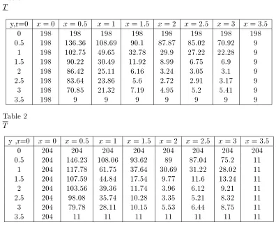
Example 4.1. Consider the one-dimensional heat equation 8

> > > > > > > > > < > > > > > > > > > :

du dt = k(d

2_u

dx2 +d 2_u

dy2)

u(0; x; y) = e0 at t = 0 and 0 x l

u(t; 0; y) = g200 = (198 + 2r; 204 4r) at x = 0 and t > 0 u(t; h; y) = e10 = (9 + r; 11 r) at h = 3:5ft; and t > 0 u(t; x; 0) = g200 = (198 + 2r; 204 4r) at y = 0 and t > 0 u(t; x; b) = e10 = (9 + r; 11 r) at b = 3:5ft and t > 0

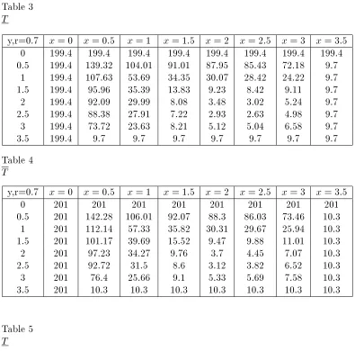
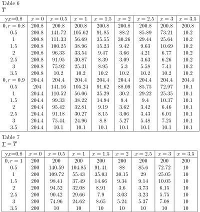
Distributions of temperature are compared for r = 0; 0:1; :::; 1 in the following Tables 1, 2,...,7.

Table 1 T

y,r=0 x = 0 x = 0:5 x = 1 x = 1:5 x = 2 x = 2:5 x = 3 x = 3:5

0 198 198 198 198 198 198 198 198

0:5 198 136:36 108:69 90:1 87:87 85:02 70:92 9

1 198 102:75 49:65 32:78 29:9 27:22 22:28 9

1:5 198 90:22 30:49 11:92 8:99 6:75 6:9 9

2 198 86:42 25:11 6:16 3:24 3:05 3:1 9

2:5 198 83:64 23:86 5:6 2:72 2:91 3:17 9

3 198 70:85 21:32 7:19 4:95 5:2 5:41 9

3:5 198 9 9 9 9 9 9 9

Table 2 T

y ,r=0 x = 0 x = 0:5 x = 1 x = 1:5 x = 2 x = 2:5 x = 3 x = 3:5

0 204 204 204 204 204 204 204 204

0:5 204 146:23 108:06 93:62 89 87:04 75:2 11

1 204 117:78 61:75 37:64 30:69 31:22 28:02 11

1:5 204 107:59 44:84 17:54 9:77 11:6 13:24 11

2 204 103:56 39:36 11:74 3:96 6:12 9:21 11

2:5 204 98:08 35:74 10:28 3:35 5:21 8:32 11

3 204 79:78 28:11 10:15 5:53 6:44 8:75 11

3:5 204 11 11 11 11 11 11 11

(13)

Table 3 T

y,r=0.7 x = 0 x = 0:5 x = 1 x = 1:5 x = 2 x = 2:5 x = 3 x = 3:5

0 199:4 199:4 199:4 199:4 199:4 199:4 199:4 199:4

0:5 199:4 139:32 104:01 91:01 87:95 85:43 72:18 9:7

1 199:4 107:63 53:69 34:35 30:07 28:42 24:22 9:7

1:5 199:4 95:96 35:39 13:83 9:23 8:42 9:11 9:7

2 199:4 92:09 29:99 8:08 3:48 3:02 5:24 9:7

2:5 199:4 88:38 27:91 7:22 2:93 2:63 4:98 9:7

3 199:4 73:72 23:63 8:21 5:12 5:04 6:58 9:7

3:5 199:4 9:7 9:7 9:7 9:7 9:7 9:7 9:7

Table 4 T

y,r=0.7 x = 0 x = 0:5 x = 1 x = 1:5 x = 2 x = 2:5 x = 3 x = 3:5

0 201 201 201 201 201 201 201 201

0:5 201 142:28 106:01 92:07 88:3 86:03 73:46 10:3

1 201 112:14 57:33 35:82 30:31 29:67 25:94 10:3

1:5 201 101:17 39:69 15:52 9:47 9:88 11:01 10:3

2 201 97:23 34:27 9:76 3:7 4:45 7:07 10:3

2:5 201 92:72 31:5 8:6 3:12 3:82 6:52 10:3

3 201 76:4 25:66 9:1 5:33 5:69 7:58 10:3

3:5 201 10:3 10:3 10:3 10:3 10:3 10:3 10:3

Table 5 T

y,r=0.8 x = 0 x = 0:5 x = 1 x = 1:5 x = 2 x = 2:5 x = 3 x = 3:5

0; r = 0:8 199:6 199:6 199:6 199:6 199:6 199:6 199:6 199:6

0:5 199:6 139:75 104:29 91:14 87:97 85:49 72:36 9:8

1 199:6 108:32 54:28 34:58 30:1 28:61 24:5 9:8

1:5 199:6 96:78 36:09 14:11 9:27 8:66 9:42 9:8

2 199:6 92:9 30:69 8:36 3:52 3:26 5:55 9:8

2:5 199:6 89:06 28:5 7:45 2:97 2:83 5:23 9:8

3 199:6 74:13 23:96 8:36 5:18 5:15 6:75 9:8

3:5 199:6 9:8 9:8 9:8 9:8 9:8 9:8 9:8

0; r = 0:9 199:8 199:8 199:8 199:8 199:8 199:8 199:8 199:8

0:5 199:8 140:17 104:58 91:28 87:98 85:55 72:54 9:9

1 199:8 109:02 54:85 34:81 30:12 28:81 24:77 9:9

1:5 199:8 97:6 36:79 14:38 9:3 8:89 9:73 9:9

2 199:8 93:71 31:38 8:63 3:55 3:49 5:85 9:9

2:5 199:8 89:74 29:08 7:68 3 3:03 5:49 9:9

3 199:8 74:54 24:29 8:5 5:2 5:26 6:91 9:9

(14)

Table 6 T

y,r=0.8 x = 0 x = 0:5 x = 1 x = 1:5 x = 2 x = 2:5 x = 3 x = 3:5

0; r = 0:8 200:8 200:8 200:8 200:8 200:8 200:8 200:8 200:8

0:5 200:8 141:72 105:62 91:85 88:2 85:89 73:21 10:2

1 200:8 111:33 56:69 35:55 30:26 29:44 25:64 10:2

1:5 200:8 100:25 38:96 15:23 9:42 9:63 10:69 10:2

2 200:8 96:33 33:54 9:47 3:66 4:21 6:77 10:2

2:5 200:8 91:95 30:87 8:39 3:09 3:63 6:26 10:2

3 200:8 75:92 25:31 8:95 5:3 5:58 7:41 10:2

3:5 200:8 10:2 10:2 10:2 10:2 10:2 10:2 10:2

0; r = 0:9 204:4 204:4 204:4 204:4 204:4 204:4 204:4 204:4

0:5 204 141:16 105:24 91:62 88:09 85:75 72:97 10:1

1 204:4 110:52 56:06 35:29 30:2 29:22 25:35 10:1

1:5 204:4 99:33 38:22 14:94 9:4 9:4 10:37 10:1

2 204:4 95:42 32:81 9:19 3:62 3:42 6:46 10:1

2:5 204:4 91:18 30:27 8:15 3:06 3:43 6:01 10:1

3 204:4 75:44 24:96 8:8 5:27 5:48 7:25 10:1

3:5 204:4 10:1 10:1 10:1 10:1 10:1 10:1 10:1

Table 7 T = T

y,r=0.8 x = 0 x = 0:5 x = 1 x = 1:5 x = 2 x = 2:5 x = 3 x = 3:5

0; r = 1 200 200 200 200 200 200 200 200

0:5 200 140:59 104:85 91:41 88 85:6 72:72 10

1 200 109:72 55:43 35:03 30:15 29 25:05 10

1:5 200 98:41 37:49 14:66 9:34 9:14 10:05 10

2 200 94:52 32:08 8:91 3:6 3:73 6:15 10

2:5 200 90:42 29:66 7:9 3:03 3:23 5:75 10

3 200 74:96 24:62 8:65 5:24 5:37 7:08 10

3:5 200 10 10 10 10 10 10 10

We see that the solution of a PDE is dependent on the selection of the derivative: whether it is (i)-dierentiable or (ii)-dierentiable. In this example, the solution of a PDE is of the case(1) type.

5 Conclusion

In this paper, we proposed a numerical method for solving a two-dimensional heat equa-tion. This numerical method is based on the denition of the strongly generalized deriva-tive.

References

(15)

[2] T. Allahviranloo, N. Ahmady, E. Ahmady, Numerical solution of fuzzy dierential equations by predictor-corrector method, Information Sciences 177/7 (2007) 1633-1647.

[3] T. Allahviranloo, Dierence methods for fuzzy partial dierential equations, Compu-tational methods in appliead mathematics 2 (3) (2002) 1-10.

[4] G. A. Anastassiou, S.G. Gal, On a fuzzy trigonometric approximation theorem of Weierstrass-type, Journal of Fuzzy Mathematics 9 (2004) 701-708.

[5] B. Bede, S. G. Gal, Almost periodic fuzzy -number-valued functions, Fuzzy Sets and Systems 147 (2004) 385-403.

[6] B. Bede, S. G. Gal, Generalizations of the dierentiability of fuzzy-number-valued functions with applications to fuzzy dierential equations, Fuzzy Sets and Systems 151 (2005) 581-599.

[7] B. Bede, I. Rudas, A. Bencsik, First order linear fuzzy dierential equations under generalized dierentiablity, Information sciences 177 (2006) 3627-3635.

[8] J. J. Buckly, Thomas Feuring, Introduction to fuzzy partial dierential equations, Fuzzy Sets and Systems 105 (1999) 241-248.

[9] S. S. L. Chang and L.A. Zadeh, On fuzzy mapping and control, IEEE Trans. Systems Man Cybernet. 2 (1972) 30-34.

[10] Y. Chalco-Cano, H. Roman-Flores, On new solutions of fuzzy dierential equations . Chaos, Solitons and Fractals (2006)1016-1043.

[11] C. K. Chen and S. H. Ho, Solving partial dierential equations by two-dimensional dierential transform method, Applied Mathematics and Computation 106 (1999) 171-179.

[12] M. Dehghan, A nite dierence method for a non-local boundary value problem for two-dimensional heat equation, Applied Mathematics and Computation 112 (2000) 133-142.

[13] D. Dubios, H. Prade, Fuzzy numbers: an overview, in: J. Bezdek (Ed.), Analysis of Fuzzy Information, CRC Press, (1987) 112-148.

[14] M. Friedman, M. Ming, A. Kandel, Numerical solution of fuzzy dierential and inte-gral equations, Fuzzy Sets and Systems 106 (1999) 35-48.

[15] S. G. Gal, Approximation theory in fuzzy setting, in: G.A. Anastassiou (Ed.), Hand-book of Analytic-Computational Methods in Applied Mathematics, Chapman Hall CRC Press, (2000) 617-666.

[16] R. Goetschel, W. Voxman, Elementary calculus, Fuzzy Sets and Systems 18 (1986) 31-43.

(16)

[18] M. J. Jang, C. L. Chen and Y. C. Liy, On solving the initial-value problems using the dierential transformation method, Applied Mathematics and Computation 115 (2000) 145-160.

[19] O. Kaleva, Fuzzy dierential equations, Fuzzy Sets and Systems 24 (1987) 301-317. [20] M. Ma, M. Friedman, A. Kandel, Numerical solution of fuzzy dierential equations,

Fuzzy Sets and Systems 105 (1999) 133-138.

[21] W. Menda, Linear fuzzy dierential equation systems on R, J. Fuzzy Systems Math. 2 (1988) 51-56 (in Chinese).

[22] M. L. Puri, D. Ralescu, Fuzzy random variables, Journal of Mathematical Analysis and Applications 114 (1986) 409-422

[23] M. L. Puri, D. Ralescu, Dierential for fuzzy function, Journal of Mathematical Analysis and Applications 91 (1983) 552-558.

[24] S. Seikkala, On the fuzzy initial value problem, Fuzzy Sets and Systems 24 (1987) 319-330.

[25] J. K. Zhou, Dierential transformation and its applications for Electrical Circuits, Huarjung University Press, (1986).