Target-Side Context for Discriminative Models in Statistical Machine
Translation
Aleˇs Tamchyna1,2, Alexander Fraser1, Ondˇrej Bojar2 and Marcin Junczys-Dowmunt3 1LMU Munich, Munich, Germany
2Charles University in Prague, Prague, Czech Republic 3Adam Mickiewicz University in Pozna´n, Pozna´n, Poland
{tamchyna,bojar}@ufal.mff.cuni.cz [email protected] [email protected]
Abstract
Discriminative translation models utiliz-ing source context have been shown to help statistical machine translation perfor-mance. We propose a novel extension of this work using target context information. Surprisingly, we show that this model can be efficiently integrated directly in the de-coding process. Our approach scales to large training data sizes and results in con-sistent improvements in translation qual-ity on four language pairs. We also pro-vide an analysis comparing the strengths of the baseline source-context model with our extended source-context and target-context model and we show that our ex-tension allows us to better capture mor-phological coherence. Our work is freely available as part of Moses.
1 Introduction
Discriminative lexicons address some of the core challenges of phrase-based MT (PBMT) when translating to morphologically rich languages, such as Czech, namely sense disambiguation and morphological coherence. The first issue is se-mantic: given a source word or phrase, which of its possible meanings (i.e., which stem or lemma) should we choose? Previous work has shown that this can be addressed using a discriminative lex-icon. The second issue has to do with morphol-ogy (and syntax): given that we selected the cor-rect meaning, which of its inflected surface forms is appropriate? In this work, we integrate such a model directly into the SMT decoder. This enables our classifier to extract features not only from the full source sentence but also from a limited target-side context. This allows the model to not only
help with semantics but also to improve morpho-logical and syntactic coherence.
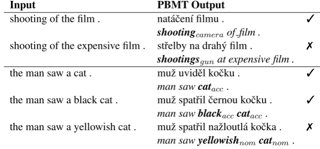
Forsense disambiguation, source context is the main source of information, as has been shown in previous work (Vickrey et al., 2005), (Carpuat and Wu, 2007), (Gimpel and Smith, 2008) inter alia. Consider the first set of examples in Figure 1, pro-duced by a strong baseline PBMT system. The English word “shooting” has multiple senses when translated into Czech: it may either be the act of firing a weapon or making a film. When the cue word “film” is close, the phrase-based model is able to use it in one phrase with the ambiguous “shooting”, disambiguating correctly the transla-tion. When we add a single word in between, the model fails to capture the relationship and the most frequent sense is selected instead. Wider source context information is required for correct disam-biguation.
While word/phrase senses can usually be in-ferred from the source sentence, the correct se-lection of surface formsrequires also information from the target. Note that we can obtain some
information from the source. For example, an English subject is often translated into a Czech subject; in which case the Czech word should be in nominative case. But there are many deci-sions that happen during decoding which deter-mine morphological and syntactic properties of words – verbs can have translations which differ in valency frames, they may be translated in either active or passive voice (in which case subject and object would be switched), nouns may have dif-ferent possible translations which differ in gender, etc.
The correct selection of surface forms plays a crucial role in preserving meaning in morpho-logically rich languages because it is morphol-ogy rather than word order that expresses rela-tions between words. (Word order tends to be
Input PBMT Output
shooting of the film . nat´aˇcen´ı filmu . 3
shootingcameraof film .
shooting of the expensive film . stˇrelby na drah´y film . 7
shootingsgunat expensive film .
the man saw a cat . muˇz uvidˇel koˇcku . 3
man sawcatacc.
the man saw a black cat . muˇz spatˇril ˇcernou koˇcku . 3
man sawblackacccatacc.
the man saw a yellowish cat . muˇz spatˇril naˇzloutl´a koˇcka . 7
[image:2.595.135.458.64.214.2]man sawyellowishnomcatnom.
Figure 1: Examples of problems of PBMT: lexical selection and morphological coherence. Each trans-lation has a corresponding gloss in italics.
relatively free and driven more by semantic con-straints rather than syntactic concon-straints.)
The language model is only partially able to capture this phenomenon. It has a limited scope and perhaps more seriously, it suffers from data sparsity. The units captured by both the phrase ta-ble and the LM are mere sequences of words. In order to estimate their probability, we need to ob-serve them in the training data (many times, if the estimates should be reliable). However, the num-ber of possiblen-grams grows exponentially as we increasen, leading to unrealistic requirements on training data sizes. This implies that the current models can (and often do) miss relationships be-tween words even within their theoretical scope.
The second set of sentences in Figure 1 demon-strates the problem of data sparsity for morpho-logical coherence. While the phrase-based sys-tem can correctly transfer the morphological case of “cat” and even “black cat”, the less usual “yellowish cat” is mistranslated into nominative case, even though the correct phrase “yellowish||| naˇzloutlou” exists in the phrase table. A model with a suitable representation of two preceding words could easily infer the correct case in this example.
Our contributions are the following:
• We show that the addition of a feature-rich discriminative model significantly improves translation quality even for large data sizes and that target-side context information con-sistently further increases this improvement. • We provide an analysis of the outputs which
confirms that source-context features indeed help with semantic disambiguation (as is well
known). Importantly, we also show that our novel use of target context improves morpho-logical and syntactic coherence.
• In addition to extensive experimentation on translation from English to Czech, we also evaluate English to German, English to Pol-ish and EnglPol-ish to Romanian tasks, with im-provements on translation quality in all tasks, showing that our work is broadly applicable.
• We describe several optimizations which al-low target-side features to be used efficiently in the context of phrase-based decoding.
• Our implementation is freely available in the widely used open-source MT toolkit Moses, enabling other researchers to explore dis-criminative modelling with target context in MT.
2 Discriminative Model with Target-Side Context
Several different ways of using feature-rich mod-els in MT have been proposed, see Section 6. We describe our approach in this section.
2.1 Model Definition
Letf be the source sentence andeits translation. We denote source-side phrases (given a particular phrasal segmentation)( ¯f1, . . . ,fm¯ ) and the
indi-vidual words(f1, . . . , fn). We use a similar nota-tion for target-side words/phrases.
For simplicity, let eprev, eprev−1 denote the
P(e|f)∝ Y
( ¯ei,f¯i)∈(e,f)
P( ¯ei|f¯i, f, eprev, eprev−1)
(1) The probability of a translation is the product of phrasal translation probabilities which are condi-tioned on the source phrase, the full source sen-tence and several previous target words.
LetGEN( ¯fi)be the set of possible translations of the source phrase fi¯ according to the phrase table. We also define a “feature vector” function
fv( ¯ei,f¯i, f, eprev, eprev−1)which outputs a vector
of features given the phrase pair and its context information. We also have a vector of feature weightswestimated from the training data. Then our model defines the phrasal translation probabil-ity simply as follows:
P( ¯ei|f¯i, f, eprev, eprev−1)
= Pexp(w·fv( ¯ei,fi, f, eprev, eprev¯ −1)) ¯
e0∈GEN( ¯fi)exp(w·fv(¯e
0,fi, f, eprev, eprev¯ −1))
(2)
This definition implies that we have to locally normalize the classifier outputs so that they sum to one.
In PBMT, translations are usually scored by a log-linear model. Our classifier produces a single score (the conditional phrasal probability) which we add to the standard log-linear model as an addi-tional feature. The MT system therefore does not have direct access to theclassifierfeatures, only to the final score.
2.2 Global Model
We use the Vowpal Wabbit (VW) classifier1in this work. Tamchyna et al. (2014) already integrated VW into Moses. We started from their implemen-tation in order to carry out our work. Classifier features are divided into two “namespaces”:
• S.Features that do not depend on the current phrasal translation (i.e., source- and target-context features).
• T.Features of the current phrasal translation. We make heavy use of feature processing avail-able in VW, namely quadratic feature expansions
1http://hunch.net/˜vw/
and label-dependent features. When generating features for a particular set of translations, we first create the shared features (in the namespace S). These only depend on (source and target) context and are therefore constant for all possible transla-tions of a given phrase. (Note that target-side con-text naturally depends on the current partial trans-lation. However, when we process the possible translations for a single source phrase, the target context is constant.)
Then for each translation, we extract its features and store them in the namespaceT. Note that we do not provide a label (or class) to VW – it is up to thesetranslationfeatures to describe the target phrase. (And this is what is referred to as “label-dependent features” in VW.)
Finally, we add the Cartesian product between the two namespaces to the feature set: every
sharedfeature is combined with everytranslation
feature.
This setting allows us to train only a single, global model with powerful feature sharing. For example, thanks to the label-dependent format, we can decompose both the source phrase and the tar-get phrase into words and have features such as
s cat t koˇcka which capture phrase-internal word translations. Predictions for rare phrase pairs are then more robust thanks to the rich statistics collected for these word-level feature pairs.
2.3 Extraction of Training Examples
Discriminative models in MT are typically trained by creating one training instance per extracted phrase from the entire training data. The target side of the extracted phrase is a positive label, and all other phrases observed aligned to the extracted phrase (anywhere in the training data) are the neg-ative labels.
We train our model in a similar fashion: for each sentence in the parallel training data, we look at all possible phrasal segmentations. Then for each source span, we create a training example. We ob-tain the set of possible translationsGEN( ¯f)from the phrase table. Because we do not have actual classes, each translation is defined by its label-dependent features and we associate a loss with it: 0 loss for the correct translation and 1 for all others.
Feature Type Czech GermanConfigurations Polish, Romanian Source Indicator f, l, l+t, t f, l, l+t, t l, t
Source Internal f, f+a, f+p, l, l+t, t, a+p f, f+a, f+p, l, l+t, t, a+p l, l+a, l+p, t, a+p Source Context f (-3,3), l (-3,3), t (-5,5) f (-3,3), l (-3,3), t (-5,5) l (-3,3), t (-5,5)
Target Context f (2), l (2), t (2), l+t (2) f (2), l (2), t (2), l+t (2) l (2), t (2) Bilingual Context — l+t/l+t (2) l+t/l+t (2)
[image:4.595.95.507.63.186.2]Target Indicator f, l, t f, l, t l, t Target Internal f, l, l+t, t f, l, l+t, t l, t
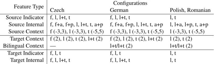
Table 1: List of used feature templates. Letter abbreviations refer to word factors: f (form), l (lemma), t (morphological tag), a (analytical function), p (lemma of dependency parent). Numbers in parentheses indicate context size.
over-fitting. We look at phrase counts and co-occurrence counts in the training data, we subtract one from the number of occurrences for the cur-rent source phrase, target phrase and the phrase pair. If the count goes to zero, we skip the train-ing example. Without this technique, the classifier might learn to simply trust very long phrase pairs which were extracted from the same training sen-tence.
For target-side context features, we simply use the true (gold) target context. This leads to train-ing which is similar to language model estima-tion; this model is somewhat similar to the neural joint model for MT (Devlin et al., 2014), but in our case implemented using a linear (maximum-entropy-like) model.
2.4 Training
We use Vowpal Wabbit in the--csoaa ldf mc
setting which reduces our multi-class problem to one-against-all binary classification. We use the logistic loss as our objective. We experimented with various settings of L2 regularization but were not able to get an improvement over not using reg-ularization at all. We train each model with 10 iterations over the data.
We evaluate all of our models on a held-out set. We use the same dataset as for MT system tuning because it closely matches the domain of our test set. We evaluate model accuracy after each pass over the training data to detect over-fitting and we select the model with the highest held-out accu-racy.
2.5 Feature Set
Our feature set requires some linguistic process-ing of the data. We use the factored MT settprocess-ing
(Koehn and Hoang, 2007) and we represent each type of information as an individual factor. On the source side, we use the word surface form, its lemma, morphological tag, analytical function (such asSubj for subjects) and the lemma of the parent node in the dependency parse tree. On the target side, we only use word lemmas and mor-phological tags.
Table 1 lists our feature sets for each language pair. We implementedindicator features for both the source and target side; these are simply con-catenations of the words in the current phrase into a single feature. Internalfeatures describe words within the current phrase. Context features are extracted either from a window of a fixed size around the current phrase (on the source side) or from a limited left-hand side context (on the tar-get side).Bilingual contextfeatures are concatena-tions of target-side context words and their source-side counterparts (according to word alignment); these features are similar to bilingual tokens in bilingual LMs (Niehues et al., 2011). Each of our feature types can be configured to look at any in-dividual factors or their combinations.
The features in Table 1 are divided into three sets. The first set contains label-independent (=shared) features which only depend on the source sentence. The second set contains shared features which depend on target-side context; these can only be used when VW is applied dur-ing decoddur-ing. We use target context size two in all our experiments.2 Finally, the third set con-tains label-dependent features which describe the currently predicted phrasal translation.
2In preliminary experiments we found that using a single
Going back to the examples from Figure 1, our model can disambiguate the translation of “shoot-ing” based on the source-context features (either the full form or lemma). For the morphologi-cal disambiguation of the translation of “yellow-ish cat”, the model has access to the morpholog-ical tags of the preceding target words which can disambiguate the correct morphological case.
We used slightly different subsets of the full fea-ture set for different languages. In particular, we left out surface form features and/or bilingual fea-tures in some settings because they decreased per-formance, presumably due to over-fitting.
3 Efficient Implementation
Originally, we assumed that using target-side con-text features in decoding would be too expen-sive, considering that we would have to query our model roughly as often as the language model. In preliminary experiments, we therefore focused on n-best list re-ranking. We obtained small gains but all of our results were substantially worse than with the integrated model, so we omit them from the paper.
We find that decoding with a feature-rich target-context model is in fact feasible. In this section, we describe optimizations at different stages of our pipeline which make training and inference with our model practical.
3.1 Feature Extraction
We implemented the code for feature extraction only once; identical code is used at training time and in decoding. At training time, the generated features are written into a file whereas at test time, they are fed directly into the classifier via its li-brary interface.
This design decision not only ensures consis-tency in feature representation but also makes the process of feature extraction efficient. In training, we are easily able to use multi-threading (already implemented in Moses) and because the process-ing of trainprocess-ing data is a trivially parallel task, we can also use distributed computation and run sep-arate instances of (multi-threaded) Moses on sev-eral machines. This enables us to easily produce training files from millions of parallel sentences within a short time.
3.2 Model Training
VW is a very fast classifier by itself, however for very large data, its training can be further sped up by using parallelization. We take advantage of its implementation of the AllReduce scheme which we utilize in a grid engine environment. We shuf-fle and shard the data and then assign each shard to a worker job. With AllReduce, there is a master job which synchronizes the learned weight vector with all workers. We have compared this approach with the standard single-threaded, single-process training and found that we obtain identical model accuracy. We usually use around 10-20 training jobs.
This way, we can process our large training files quickly and train the full model (using multi-ple passes over the data) within hours; effectively, neither feature extraction nor model training be-come a significant bottleneck in the full MT sys-tem training pipeline.
3.3 Decoding
In phrase-based decoding, translation is generated from left to right. At each step, a partial transla-tion (initially empty) is extended by translating a previously uncovered part of the source sentence. There are typically many ways to translate each source span, which we refer to as translation op-tions. The decoding process gradually extends the generated partial translations until the whole source sentence is covered; the final translation is then the full translation hypothesis with the high-est model score. Various pruning strategies are ap-plied to make decoding tractable.
Evaluating a feature-rich classifier during de-coding is a computationally expensive operation. Because the features in our model depend on target-side context, the feature function which computes the classifier score cannot evaluate the translation options in isolation (independently of the partial translation). Instead, similarly to a lan-guage model, it needs to look at previously gener-ated words. This also entails maintaining a state which captures the required context information.
A naive integration of the classifier would sim-ply generate all source-context features, all target-context features and all features describing the translation option each time a partial hypothesis is evaluated. This is a computationally very expen-sive approach.
which make decoding reasonably fast. Decoding a single sentence with the naive approach takes 13.7 seconds on average. With our optimization, this average time is reduced to 2.9 seconds, i.e. almost by 80 per cent. The baseline system produces a translation in 0.8 seconds on average.
Separation of source-context and target-context evaluation. Because we have a linear model, the final score is simply the dot product be-tween a weight vector and a (sparse) feature vec-tor. It is therefore trivial to separate it into two components: one that only contains features which depend on the source context and the other with target context features. We can pre-compute the source-context part of the score before decoding (once we have all translation options for the given sentence). We cache these partial scores and when the translation option is evaluated, we add the par-tial score of the target-context features to arrive at the final classifier score.
Caching of feature hashes. VW uses feature hashing internally and it is possible to obtain the hash of any feature that we use. When we en-counter a previously unseen target context (=state) during decoding, we store the hashes of extracted features in a cache. Therefore for each context, we only run the expensive feature extraction once. Similarly, we pre-compute feature hash vectors for all translation options.
Caching of final results. Our classifier locally normalizes the scores so that the probabilities of translations for a given span sum to one. This cannot be done without evaluating all translation options for the span at the same time. Therefore, when we get a translation option to be scored, we fetch all translation options for the given source span and evaluate all of them. We then normalize the scores and add them to a cache of final results. When the other translation options come up, their scores are simply fetched from the cache. This can also further save computation when we get into a previously seen state (from the point of view of our classifier) and we evaluate the same set of transla-tion optransla-tions in that state; we will simply find the result in cache in such cases.
When we combine all of these optimizations, we arrive at the query algorithm shown in Figure 2.
4 Experimental Evaluation
We run the main set of experiments on English to Czech translation. To verify that our method is
functionEVALUATE(t, s)
span =t.getSourceSpan()
if notresultCache.has(span,s)then
scores = ()
if notstateCache.has(s)then
stateCache[s] = CtxFeatures(s)
end if
for allt0 ←span.tOpts()do
srcScore = srcScoreCache[t0]
c.addFeatures(stateCache[s]) c.addFeatures(translationCache[t0])
tgtScore =c.predict()
scores[t0] = srcScore + tgtScore end for
normalize(scores)
resultCache[span,s] = scores
end if
returnresultCache[span,s][t]
end function
Figure 2: Algorithm for obtaining classifier pre-dictions during decoding. The variabletstands for the current translation,sis the current state andc is an instance of the classifier.
applicable to other language pairs, we also present experiments in English to German, Polish, and Ro-manian.
In all experiments, we use Treex (Popel and ˇZabokrtsk´y, 2010) to lemmatize and tag the source data and also to obtain dependency parses of all English sentences.
4.1 English-Czech Translation
As parallel training data, we use (subsets of) the CzEng 1.0 corpus (Bojar et al., 2012). For tuning, we use the WMT13 test set (Bojar et al., 2013) and we evaluate the systems on the WMT14 test set (Bojar et al., 2014). We lemmatize and tag the Czech data using Morphodita (Strakov´a et al., 2014).
Our baseline system is a standard phrase-based Moses setup. The phrase table in both cases is fac-tored and outputs also lemmas and morphological tags. We train a 5-gram LM on the target side of parallel data.
We evaluate three settings in our experiments:
• baseline – vanilla phrase-based system,
• +target – our classifier with both source-context and target-source-context features.
For each of these settings, we vary the size of the training data for our classifier, the phrase ta-ble and the LM. We experiment with three dif-ferent sizes: small (200 thousand sentence pairs), medium (5 million sentence pairs), and full (the whole CzEng corpus, over 14.8 million sentence pairs).
For each setting, we run system weight opti-mization (tuning) using minimum error rate train-ing (Och, 2003) five times and report the aver-age BLEU score. We use MultEval (Clark et al., 2011) to compare the systems and to determine whether the differences in results are statistically significant. We always compare the baseline with +source and +source with +target.
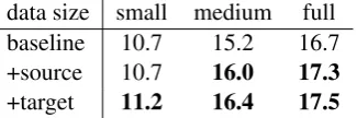
Table 2 shows the obtained results. Statisti-cally significant differences (α=0.01) are marked in bold. The source-context model does not help in the small data setting but brings a substantial im-provement of 0.7-0.8 BLEU points for the medium and full data settings, which is an encouraging re-sult.
Target-side context information allows our model to push the translation quality further: even for the small data setting, it brings a substantial improvement of 0.5 BLEU points and the gain re-mains significant as the data size increases. Even in the full data setting, target-side features improve the score by roughly 0.2 BLEU points.
Our results demonstrate that feature-rich mod-els scale to large data size both in terms of techni-cal feasibility and of translation quality improve-ments. Target side information seems consistently beneficial, adding further 0.2-0.5 BLEU points on top of the source-context model.
data size small medium full baseline 10.7 15.2 16.7 +source 10.7 16.0 17.3
[image:7.595.102.265.582.636.2]+target 11.2 16.4 17.5
Table 2: BLEU scores obtained on the WMT14 test set. We report the performance of the baseline, the source-context model and the full model.
Intrinsic Evaluation. For completeness, we report intrinsic evaluation results. We evaluate the classifier on a held-out set (WMT13 test set) by extracting all phrase pairs from the test in-put aligned with the test reference (similarly as
we would in training) and scoring each phrase pair (along with other possible translations of the source phrase) with our classifier. An instance is classified correctly if the true translation obtains the highest score by our model. A baseline which always chooses the most frequent phrasal trans-lation obtains accuracy of 51.5. For the source-context model, the held-out accuracy was 66.3, while the target context model achieved accuracy of 74.8. Note that this high difference is some-what misleading because in this setting, the target-context model has access to the true target target-context (i.e., it is cheating).
4.2 Additional Language Pairs
We experiment with translation from English into German, Polish, and Romanian.
Our English-German system is trained on the data available for the WMT14 translation task: Europarl (Koehn, 2005) and the Common Crawl corpus,3 roughly 4.3 million sentence pairs alto-gether. We tune the system on the WMT13 test set and we test on the WMT14 set. We use Tree-Tagger (Schmid, 1994) to lemmatize and tag the German data.
English-Polish has not been included in WMT shared tasks so far, but was present as a language pair for several IWSLT editions which concentrate on TED talk translation. Full test sets are only available for 2010, 2011, and 2012. The refer-ences for 2013 and 2014 were not made public. We use the development set and test set from 2010 as development data for parameter tuning. The remaining two test sets (2011, 2012) are our test data. We train on the concatenation of Europarl and WIT3(Cettolo et al., 2012), ca. 750 thousand sentence pairs. The Polish half has been tagged using WCRFT (Radziszewski, 2013) which pro-duces full morphological tags compatible with the NKJP tagset (Przepi´orkowski, 2009).
English-Romanian was added in WMT16. We train our system using the available parallel data – Europarl and SETIMES2 (Tiedemann, 2009), roughly 600 thousand sentence pairs. We tune the English-Romanian system on the official develop-ment set and we test on the WMT16 test set. We use the online tagger by Tufis et al. (2008) to pre-process the data.
Table 3 shows the obtained results. Similarly to English-Czech experiments, BLEU scores are
input: the most intensive mining took place there from 1953 to 1962 .
baseline: nejv´ıce intenzivn´ı tˇeˇzbadoˇslotam z roku 1953, aby1962 .
the most intensive miningnomthere occurredthere from 1953, in order to1962 .
+source: nejv´ıce intenzivn´ıtˇeˇzby m´ıstotam z roku 1953 do roku 1962 .
the most intensivemininggenplacethere from year 1953 until year 1962 .
+target: nejv´ıce intenzivn´ı tˇeˇzba prob´ıhala od roku 1953 do roku 1962 .
the most intensive miningnomoccurred from year 1953 until year 1962 .
Figure 3: An example sentence from the test set. Each translation has a corresponding gloss in italics. Errors are marked in bold.
language de pl (2011) pl (2012) ro baseline 15.7 12.8 10.4 19.6 +target 16.2 13.4 11.1 20.2
Table 3: BLEU scores of the baseline and of the full model for English to German, Polish, and Ro-manian.
eraged over 5 independent optimization runs. Our system outperforms the baseline by 0.5-0.7 BLEU points in all cases, showing that the method is ap-plicable to other languages with rich morphology.
5 Analysis
We manually analyze the outputs of English-Czech systems. Figure 3 shows an example sen-tence from the WMT14 test set translated by all the system variants. The baseline system makes an error in verb valency; the Czech verb “doˇslo” could be used but this verb already has an (im-plicit) subject and the translation of “mining” (“tˇeˇzba”) would have to be in a different case and at a different position in the sentence. The second error is more interesting, however: the baseline system fails to correctly identify the word sense of the particle “to” and translates it in the sense of purpose, as in “in order to”. The source-context model takes the context (span of years) into con-sideration and correctly disambiguates the trans-lation of “to”, choosing the temporal meaning. It still fails to translate the main verb correctly, though. Only the full model with target-context information is able to also correctly translate the verb and inflect its arguments according to their roles in the valency frame. The translation pro-duced by this final system in this case is almost flawless.
In order to verify that the automatically mea-sured results correspond to visible improvements in translation quality, we carried out two
annota-tion experiments. We took a random sample of 104 sentences from the test set and blindly ranked two competing translations (the selection of sen-tences was identical for both experiments). In the first experiment, we compared the baseline sys-tem with +source. In the other experiment, we compared the baseline with +target. The instruc-tions for annotation were simply to compare over-all translation quality; we did not ask the annota-tor to look for any specific phenomena. In terms of automatic measures, our selection has similar characteristics as the full test set: BLEU scores obtained on our sample are 15.08, 16.22 and 16.53 for the baseline, +source and +target respectively. In the first case, the annotator marked 52 trans-lations as equal in quality, 26 transtrans-lations pro-duced by +source were marked as better and in the remaining 26 cases, the baseline won the rank-ing. Even though there is a difference in BLEU, human annotation does not confirm this measure-ment, ranking both systems equally.
In the second experiment, 52 translations were again marked as equal. In 34 cases, +target pro-duced a better translation while in 18 cases, the baseline output won. The difference between the baseline and +target suggests that the target-context model may provide information which is useful for translation quality as perceived by hu-mans.
cor-input: destruction of the equipment means that Syria can no longer produce new chemical weapons .
+source: zniˇcen´ımzaˇr´ızen´ı znamen´a , ˇze S´yrie jiˇz nem˚uˇze vytv´aˇret nov´e chemick´e zbranˇe .
destruction ofinstrequipment means , that Syria already cannot produce new chemical weapons . +target: zniˇcen´ı zaˇr´ızen´ı znamen´a , ˇze S´yrie jiˇz nem˚uˇze vytv´aˇret nov´e chemick´e zbranˇe .
destruction ofnomequipment means , that Syria already cannot produce new chemical weapons . input: nothing like that existed , and despite that we knew far more about each other .
+source: nic takov´eho neexistovalo , a pˇresto jsme vˇedˇeli daleko v´ıc ojeden na druh´eho. nothing like that existed , and despite that we knew far more aboutonenomon other. +target: nic takov´eho neexistovalo , a pˇresto jsme vˇedˇeli daleko v´ıc o sobˇe navz´ajem .
nothing like that existed , and despite that we knew far more about each other .
input: the authors have been inspired by their neighbours .
+source: autoˇri byli inspirov´anisv´ych soused˚u.
the authors have been inspiredtheirgenneighboursgen. +target: autoˇri byli inspirov´ani sv´ymi sousedy .
the authors have been inspired theirinstrneighboursinstr.
Figure 4: Example sentences from the test set showing improvements in morphological coherence. Each translation has a corresponding gloss in italics. Errors are marked in bold.
rected by the target-context model, producing an accurate translation of the input.
6 Related Work
Discriminative models in MT have been proposed before. Carpuat and Wu (2007) trained a maxi-mum entropy classifier for each source phrase type which used source context information to disam-biguate its translations. The models did not cap-ture target-side information and they were inde-pendent; no parameters were shared between clas-sifiers for different phrases. They used a strong feature set originally developed for word sense disambiguation. Gimpel and Smith (2008) also used wider source-context information but did not train a classifier; instead, the features were in-cluded directly in the log-linear model of the de-coder. Mauser et al. (2009) introduced the “dis-criminative word lexicon” and trained a binary classifier for each target word, using as features only the bag of words (from the whole source sen-tence). Training sentences where the target word occurred were used as positive examples, other sentences served as negative examples. Jeong et al. (2010) proposed a discriminative lexicon with a rich feature set tailored to translation into mor-phologically rich languages; unlike our work, their model only used source-context features.
Subotin (2011) included target-side context in-formation in a maximum-entropy model for the prediction of morphology. The work was done within the paradigm of hierarchical PBMT and as-sumes that cube pruning is used in decoding. Their algorithm was tailored to the specific problem of passing non-local information about morphologi-cal agreement required by individual rules (such as
explicit rules enforcing subject-verb agreement). Our algorithm only assumes that hypotheses are constructed left to right and provides a general way for including target context information in the classifier, regardless of the type of features. Our implementation is freely available and can be fur-ther extended by ofur-ther researchers in the future. 7 Conclusions
We presented a discriminative model for MT which uses both source and target context infor-mation. We have shown that such a model can be used directly during decoding in a relatively efficient way. We have shown that this model consistently significantly improves the quality of English-Czech translation over a strong baseline with large training data. We have validated the ef-fectiveness of our model on several additional lan-guage pairs. We have provided an analysis show-ing concrete examples of improved lexical selec-tion and morphological coherence. Our work is available in the main branch of Moses for use by other researchers.
Acknowledgements
References
Ondˇrej Bojar, Zdenˇek ˇZabokrtsk´y, Ondˇrej Duˇsek, Pe-tra Galuˇsˇc´akov´a, Martin Majliˇs, David Mareˇcek, Jiˇr´ı Marˇs´ık, Michal Nov´ak, Martin Popel, and Aleˇs Tam-chyna. 2012. The Joy of Parallelism with CzEng 1.0. InProc. of LREC, pages 3921–3928. ELRA. Ondˇrej Bojar, Christian Buck, Chris Callison-Burch,
Christian Federmann, Barry Haddow, Philipp Koehn, Christof Monz, Matt Post, Radu Soricut, and Lucia Specia. 2013. Findings of the 2013 Work-shop on Statistical Machine Translation. In Pro-ceedings of the Eighth Workshop on Statistical
Ma-chine Translation, pages 1–44, Sofia, Bulgaria,
Au-gust. Association for Computational Linguistics. Ondˇrej Bojar, Christian Buck, Christian Federmann,
Barry Haddow, Philipp Koehn, Johannes Leveling, Christof Monz, Pavel Pecina, Matt Post, Herve Saint-Amand, Radu Soricut, Lucia Specia, and Aleˇs Tamchyna. 2014. Findings of the 2014 workshop on statistical machine translation. InProceedings of the Ninth Workshop on Statistical Machine Transla-tion, pages 12–58, Baltimore, MD, USA. Associa-tion for ComputaAssocia-tional Linguistics.
Marine Carpuat and Dekai Wu. 2007. Improving sta-tistical machine translation using word sense dis-ambiguation. InProceedings of the Conference on Empirical Methods in Natural Language Processing
(EMNLP), Prague, Czech Republic.
Mauro Cettolo, Christian Girardi, and Marcello Fed-erico. 2012. Wit3: Web inventory of transcribed and translated talks. InProceedings of the 16th
Con-ference of the European Association for Machine
Translation (EAMT), pages 261–268, Trento, Italy,
May.
Jonathan H. Clark, Chris Dyer, Alon Lavie, and Noah A. Smith. 2011. Better hypothesis testing for statistical machine translation: Controlling for opti-mizer instability. InProceedings of the 49th Annual Meeting of the Association for Computational Lin-guistics: Human Language Technologies: Short
Pa-pers - Volume 2, HLT ’11, pages 176–181,
Strouds-burg, PA, USA. Association for Computational Lin-guistics.
Jacob Devlin, Rabih Zbib, Zhongqiang Huang, Thomas Lamar, Richard M. Schwartz, and John Makhoul. 2014. Fast and robust neural network joint models for statistical machine translation. In Proceedings of the 52nd Annual Meeting of the Association for Computational Linguistics, ACL 2014, June 22-27,
2014, Baltimore, MD, USA, Volume 1: Long Papers,
pages 1370–1380.
K. Gimpel and N. A. Smith. 2008. Rich Source-Side Context for Statistical Machine Translation. Colum-bus, Ohio.
Minwoo Jeong, Kristina Toutanova, Hisami Suzuki, and Chris Quirk. 2010. A discriminative lexicon
model for complex morphology. InThe Ninth Con-ference of the Association for Machine Translation
in the Americas. Association for Computational
Lin-guistics, November.
Philipp Koehn and Hieu Hoang. 2007. Factored trans-lation models. In Proceedings of the 2007 Joint Conference on Empirical Methods in Natural guage Processing and Computational Natural
Lan-guage Learning (EMNLP-CoNLL), pages 868–876,
Prague, Czech Republic, June. Association for Com-putational Linguistics.
Philipp Koehn. 2005. Europarl: A Parallel Corpus for Statistical Machine Translation. InConference Proceedings: the tenth Machine Translation Sum-mit, pages 79–86, Phuket, Thailand. AAMT, AAMT. Arne Mauser, Sasa Hasan, and Hermann Ney. 2009. Extending Statistical Machine Translation with Dis-criminative and Trigger-Based Lexicon Models. pages 210–218, Suntec, Singapore.
Jan Niehues, Teresa Herrmann, Stephan Vogel, and Alex Waibel. 2011. Wider Context by Using Bilin-gual Language Models in Machine Translation. In Proceedings of the Sixth Workshop on Statistical
Machine Translation, pages 198–206, Edinburgh,
Scotland, July. Association for Computational Lin-guistics.
Franz Josef Och. 2003. Minimum Error Rate Training in Statistical Machine Translation. InProc. of ACL, pages 160–167, Sapporo, Japan. ACL.
Martin Popel and Zdenˇek ˇZabokrtsk´y. 2010. Tec-toMT: Modular NLP Framework. In Hrafn Lofts-son, Eirikur R¨ognvaldsLofts-son, and Sigrun Helgadottir, editors,IceTAL 2010, volume 6233 ofLecture Notes
in Computer Science, pages 293–304. Iceland
Cen-tre for Language Technology (ICLT), Springer. Adam Przepi´orkowski. 2009. A comparison of
two morphosyntactic tagsets of Polish. In Violetta Koseska-Toszewa, Ludmila Dimitrova, and Roman Roszko, editors, Representing Semantics in Digital Lexicography: Proceedings of MONDILEX Fourth
Open Workshop, pages 138–144, Warsaw.
Adam Radziszewski. 2013. A tiered CRF tagger for Polish. In Robert Bembenik, Lukasz Skonieczny, Henryk Rybinski, Marzena Kryszkiewicz, and Marek Niezgodka, editors, Intelligent Tools for
Building a Scientific Information Platform, volume
467 ofStudies in Computational Intelligence, pages 215–230. Springer.
Helmut Schmid. 1994. Probabilistic part-of-speech tagging using decision trees. InInternational
Con-ference on New Methods in Language Processing,
pages 44–49, Manchester, UK.
In Proceedings of 52nd Annual Meeting of the As-sociation for Computational Linguistics: System
Demonstrations, pages 13–18, Baltimore,
Mary-land, June. Association for Computational Linguis-tics.
Michael Subotin. 2011. An exponential translation model for target language morphology. InThe 49th Annual Meeting of the Association for Computa-tional Linguistics: Human Language Technologies, Proceedings of the Conference, 19-24 June, 2011,
Portland, Oregon, USA, pages 230–238.
Aleˇs Tamchyna, Fabienne Braune, Alexander Fraser, Marine Carpuat, Hal Daum´e III, and Chris Quirk. 2014. Integrating a discriminative clas-sifier into phrase-based and hierarchical decoding.
The Prague Bulletin of Mathematical Linguistics,
101:29–41.
J¨org Tiedemann. 2009. News from OPUS - A col-lection of multilingual parallel corpora with tools and interfaces. In N. Nicolov, K. Bontcheva, G. Angelova, and R. Mitkov, editors, Recent
Advances in Natural Language Processing,
vol-ume V, pages 237–248. John Benjamins, Amster-dam/Philadelphia, Borovets, Bulgaria.
Dan Tufis, Radu Ion, Alexandru Ceausu, and Dan Ste-fanescu. 2008. Racai’s linguistic web services.
In Proceedings of the International Conference on
Language Resources and Evaluation, LREC 2008,
26 May - 1 June 2008, Marrakech, Morocco.
D. Vickrey, L. Biewald, M. Teyssier, and D. Koller. 2005. Word-Sense Disambiguation for Machine Translation. InConference on Empirical Methods
in Natural Language Processing (EMNLP),