Numerical Solution of Freholm Volterra Integral Equations by Using Scaling Function Interpolation Method

(1)

Numerical Solution of Freholm-Volterra Integral

Equations by Using Scaling Function Interpolation Method

Yousef Al-Jarrah, En-Bing Lin

Department of Mathematics, Central Michigan University, Mt. Pleasant, USA Email: [email protected]

Received October 15,2012; revised November 15, 2012; accepted November 23, 2012

ABSTRACT

Wavelet methods are a very useful tool in solving integral equations. Both scaling functions and wavelet functions are the key elements of wavelet methods. In this article, we use scaling function interpolation method to solve Volterra in-tegral equations of the first kind, and Fredholm-Volterra inin-tegral equations. Moreover, we prove convergence theorem for the numerical solution of Volterra integral equations and Freholm-Volterra integral equations. We also present three examples of solving Volterra integral equation and one example of solving Fredholm-Volterra integral equation. Com-parisons of the results with other methods are included in the examples.

Keywords: Wavelets; Coiflets; Scaling Function Interpolation; Volterra Integral Equation; Fredholm-Volterra Integral

Equation

1. Introduction

The study of finite-dimensional linear systems is well developed. As an infinite-dimensional counter part of finite-dimensional linear systems, one can view integral equations as extensions of linear systems of algebraic equations. An integral equation maybe interpreted as an analogue of a matrix equation which is easier to solve. There are many different ways to transform integral equations to linear systems. Many different methods have been used for solving Volterra integral equations and Freholm-Velterra integral equations numerically.

In this paper, we first recall the method of scaling function interpolation. Then we solve linear Volterra integral equation of the form:

 

x

   

,

a d

f x 

_

k x t y t t (1) and Fredholm-Volterra integral equations of the form:

 

   

1

2

, d

x a b a

y x g x k x t y t t k x t y t t

 





(2)

where the functions k x t

 

, , ,k x t1

 

and k x t2

 

, are known functions and called kernels. The function f x

 

is known, and the function y t

 

is to be determined. One of the motivations in this study arose from equations in theoretical physics. In fact, there are many applica- tions in several disciplines as well. We will use scaling function interpolation method to solve integral equations. As a natural question, one would wonder any possible

convergence properties and how this method would compare with other methods. We will prove two convergence theorems and present several examples.

2. Approximation

Wavelets and scaling functions are a useful tool in approximation methods of solutions of differential and integral equations [1]. We first recall Multiresolution analysis (MRA) [2]. We assume the scaling function and wavelet function , Ψ are sufficiently smooth and satisfy MRA with compact support and Ψ has N vanishing mo- ments (defined below). The scaling function 

 

x is defined as

 

p



2j



p ,

 

p p j p

x x p x

 



   



  (3) for some coefficients



p,p Z



. By using this dilation and translation we defined a nested of sequence spaces



V j Zj, 



which is called MRA of with the following properties:

 

2

L R

1,

j j

V V j Z (4)

 

0

j j Z

V V





_

 (5)

j j Z

V





is dense in L R2

 

(6)

 

x Vj

 

2x j 1

(2)

205

then V₀







x p p



, Z



and V₀V₁ we can write

p

 

p



2



p 1,

 

p p

x x p x

 



   



  . In general,

 

p



2j



,

 

p p p j p

x x p x

 



   



  . (8) In fact, for each j we define the orthogonal subspace j

W of V_j in the subspace V_j₁, the or thogonal basis

of W_j is denoted by



, 2

j

j p p

  



, (9) and the wavelet function can be obtained by

 

x p j p,

 

x

 



  . (10) for some coefficients p. Some interesting properties of scaling and wavelet functions make wavelet method more efficiently than other methods such as spline approximations in solving an equation. A lot of computa- tional time and storage capacity can be saved since we do not require a huge number of arithmetic operations partly due to the following properties.

Vanishing moments:

 

d 0 k

x x x



, (11) and in this case the wavelet is said to have a vanishing moment of order k.

Semiorthogonality:

 

, , , , ,

; , , , .

i p x j k x i p x j k x x

p k i j p k Z

   

 

 



d 0;

(12)

The set of scaling functions

 

n j, is orthogonal at

the same level n, which means:

 

, , , , ,

, , .

n p x n k x n p x n k x x

n p k Z

   _ 





d 0;

1

(13)

Coiflet (of order L) has more symmetries and it is an orthogonal multiresolution wavelet system with,

 

d 0, 1, 2, , k

k

M 

_

x x x k  L

1

. (14)

 

d 0, 1, 2, ,

k

x x x k L



 . (15) where

 

Mk is the moment of scaling functions.

3. Scaling Function Interpolation

In MRA, any given function _{f x}

 

__{L R}2

 

_{can be}

in-terpolated by using the basis functions in the subspace j

V as follows:

 

j

 

p j p,

 

p

f x  f x 



  x (16)

where the coefficientsv _p are evaluated by using the semiorthogonality of the scaling functions (12) such that

   

 

, , d,

p j p x f x f x j p x x

   

_

 . (17)

Hence the Equation (16) becomes as follows:

 

j

 



 

d



 

, ,

j p j p p

.

f x  f x 

 

f x  x x  x

To approximate a given function f, one can use sam-pling values of f at certain points. It is proved in [3], namely, an interpolation theorem using coiflet, namely, if

 

x

 and 

 

x are sufficiently smooth and satisfy the ions (1 5) and the function

 

Equat 0)-(1 _{f x} __Ck

 

_ _, where Ω is a bounded open set in R2_, _k__N_₂_, _{j Z}_

then,

 

, ,

1

, ,

2 2 2

, j

j p j q

j j

p

p c q c

f x y f x y

x y

 

 

 

 _ _

 

 



,

(18)

where the index set is







 





p q, supp j p, supp j p, 



     .

In addition, the moment M_l satisfies

 

l, 2, , 1 Ml c l1,  N .

1,

c M and Then

 

2

1 _. 2

N N

j

j L

f f C f

 

 

  _ _

 

where C is a constant depending only on N, diameter of

Ω and

 

 , , 0, ,

 

: max , .

N N

x y m N m N m

f

f x y

x y

  



 

 



For one-dimensional analogue, we have

 

,

 

 

1

j p

f , , ,

2j 2j j p

x  f_ _ x x a b

 



(19)

and

 

 

 

2 _,

1 _.

2 N N

j L a b

f f C f



 

  _{ }

  (20)

where

 

   , , , 0, ,

 

: max .

N N

x y a b m N m

f

f x

x

 



 





4. Solutions of Linear Integral Equation

egral

4.1. Linear Volterra Integral Equation

n Formula In this section, Coiflet is used to solve linear int Equations (1) and (2), where we will explain the method in terms of matrix notation.

(3)

(19) to solve Volterra integral Equation (1). The unknown function y x

 

in Equation (1) can be expressed in term of scaling functions j p,

 

x in the subspace

j

V such that

 

,

 

j

p j p p

y x 



a  x . (21) By substituting Equation (21) into the Equation (1), we have the following system,

x

 

, 0

, d

p j p p

x

p j p

p

f x k x t a t

a k x t t t



 

  

 







 

t

(22)

To simplify the system, let

p

 

,

 

0

, d

p j

x

A x 

_

k x t  t t

Then the system (22) becomes

 

p p

 

p

f x 



a A x (23)

The coefficients can be evaluated by sub- st

.



a pp,  



eal numbers ituting the set of r







x xp, p 0,X , p ,0 X b



into the system (23), let  n, then the system (23)

n If we use the notation

can be written in the form

 

a A x a A x

 

1 1 1 2 2 1 1 1

1 1 2 2 2 2 2 2

1 1 2 2 .

n n

n n n n n

a A x f x a A x a A x a A x f x

a A x a A x a A x f x

  

   

   



1, , ,2 n



a a a  a and

n

 



A x

 



 

1 1 1 2 1

2 1 2 2 2

1 2

n

n n n

A x A x A x A x A x A

A x A x A x

 

  

 

 

 

   



 

 

   

 



1 , 2 , , n



f  f x f x  f x

equivalent to the system aA, then the system (23) is f , and the solution is

a_ _fA1_. ₂₄₎ This gives raise to coefficien

a

4.2. Linear Fredholm-Volterra Integral

To s holm-Volterra integral Equation (2), we ( ts in (23) and we obtained numerical solution to Equation (1).

Equation olve the Fred

use a similar algorithm as we use in 4.1. The unknown function can be approximated by using Equation (1) and

one can have the system of linear equations;

a B G 

where a is the vector of unknowns as we introduce in Equation (21),

   

 



g x1 ,g x2 , ,g xn



 

G and

 

1 1 1 2 1

2 1 2 2 2

1 2

n

n n n n

B x B x B x B x B x B x B

B x B x B x

 

 

  

 

 

 

   



with

and the set of

 

, 1 ,

2 ,

, d

x

p j p _a j p

b

j p a

B x x k x t x t k x t x t

 



 







x x1, , ,2  xn



is in the interval

 

a b, t sec-which one can be ly spaced. In the nex tion we will discuss the convergence for the method by deriving a convergence theorem of this numerical solution.

choose equal

5. Error Analysis

ide with the convergence rate of

, suppose that the functions In this section, we prov

our method for the numerical solution of solving linear Volterra integral equations and Freholm-Volterra integral equation respectively. We will explain the necessary conditions for the convergence.

Theorem 5.1

In Equation (1)

 

,





0,

  

,



, 0

k x t C X  c d  x X b,

 

, 0 0

k x t m  and the two functions f x

 

, y x

 

are in C



0,X



, 0 x X b, for j Z ,

 

p j p,



y xj 



a _ x



_.

If an approximate solution of the Equation (1) with coefficients obtained in (24), and the error at the point

i

x is

 

j

   

_Then

 

i i

e x  y x y xi .

1 2

j e x c _{ } ,

 

where c is a constant.

n with the following equation.

d



. (25)

At any point

Proof:

We begi

   

 

,

   

0 0

, d , p j p

p

k x t e t t k x t _   t y t _ t









x



x 



;



i j

x x j  Equation (25) becomes:

d

   

 

,

   

0 0

, d , _{p j p}

p

k x t e t t k x t    t y t  t









i



i ,

(4)

207 then

   

 

,

   

0 k x



0

, d , d

x x

p j p p

t e t t  k x t _   t y t _ t









. (26)

For

   

1

 

1

 

1

 

0

k x



0 0

, d d d

i

x

x x

t e t t 

_

m e t t m

_

e t t m e t

Then,

 

   

 

   

, 1 , 0 0 1 , 1 , d 1

, d d

d

i

i i

i

x

p i p p o

x x

p i p p o

x

p i p p o e t

k x t t y t t

m

k x t t t y t t

m

c t y t t

         _  _     _      _  _  















 _ (27)

Such that ₁

 

0 0 1 , d i x

c k x t m



_

t .

By (19), the unknown function y t

 

can be interpo-lated by using the coiflet such that:

 

2 j j p p y t  y_ _ t

 



j p, (28) If we add and subtract Equation (28) in

we get the following inequality:

Equation (27),

 

   

 

   

 

   

1 ₀ , ,

, 1 , , , 0 1 , 2 2 d 2 d 2 d 2 2 i i i i x e t 

p j p j j p

p p j p j p x i p j o p x

i p p i p

j p x i p j o p p j p

c t y t y t

p

y t

p

c y t y t t

p

y t t t

p

c y t y t t

p y              _   _ _        _ _ _     _ _ _ _  _  _ _        _ _   _ _ _  _ _       _ _ _ _  _  _ _          _ _   

















 

, 0 i x j p p t       _  





But by (20), we have that;

  

2j p p p y    _{ }   _ _   



is finite then denote it as



  , 2 0 1 2 N N

p _t _{c y}

   _       , And since j p j p

y_ _ t y

 



2. p c  _ 2j p p y   _{ }       



By using the above results and the rthonomality of the scaling functions

o

 

 

 t , we conclu e that d

 

1 0 2

1 1 1

. 2

2 2

N j j

N

e t c c y_  _ c  _{ } _c _

   

 _  _

Theorem 5.2

In Equation (2), suppose that the functions

 

   

1 ,

k x t C a b,  a b a, ,  x X b,

 

   

2 x t, C a b,  a b, , and

   

,

k y x g x are in

 

,

C a b , for j Z ,

 

,

j

p j p

y x 



a 

 

x

If an oximate solution of the Equation (2) with coefficients obtained in (24), and the rror at the point

appr

e i

x is e x

 

i y x

   

i y xi . Then

 

j

1 2

j

e x _{  }  , where β is a constant

 

Proof:

Substitute (21 get the following integral e uation

(29)

Subtracts Equation (27) from (1) and subs to get;

) into Equation (2), we q

 

1

   

, d x

j j

a

y x g x 

_

k x t y t t

   

2 , d

b _j

ak x t y t t



_

titute x by xi

 

   



 



   



 



 

1 2 1 2 ,1 ,2 , d , d , d , d d d i i i i i e x . j x _j i a b _j i a

x x _j

i

a a

b b _j

i

a a

x _j b _j

i _a i _a

y x y x

k x t y t y t t

k x t y t y t t

y t y t t y t y t t

               



(30)

(5)

 

,1

,2 , ,

,1 ,

2

d

2 2

d d

2 2

d 2

i

i i

x _j

i i a j

p p

b _j

i a j j p j j p

p p

x x

i _a j p _a j p

p p

i a j j p

p

e x y t y t y

p p

y t y t y t y t t

p p

y t y t t a y t t

p

y t y t t



  

 

 

   _ _

 

   

   _ _  _ _

   

 

   

  _ _  _  _ __

   

 

  _ _

 















, , d

2

j p j j p

p

t y t t

  _ _

 



,p

j_ j

 

, d

2

i

b b

p j a j p

p

a y  t t

  

 _  _ __

 





(31)

We use the same idea in the proof of 5.1, and obtain the following error estimate.

 

1 2

1 1 1

.

2 2 2

j j j

i

e x   _{ }   _{ }  _{ }

     

Remark

Here we discuss only the case when the kernel function k x t

 

,

any given

is positive. We can generalize our method for continuous function k x t

 

, in Equation (1);

1) If k x t

 

, e theore

is positive, we have obtained the con- vergenc m.

2) If k x t

 

, is negative then let k x t

 

,  S x t

 

, , and we can apply

   

0 , d

x then the is positive our me

function thod for t

 

,

S x t

he equation f x

 



_

S x t y t uation (1).

t

which m s

n be written as a sum of two positive

, tion (1) becomes

the Eq has the sa e solution a

3) If the function k x t

 

, is neither of the above two cases, the function k x t

 

, ca

functions where

 

,

 

,



 



k x t _k x t _{ }k x t Then Equa

 

₀x

   

, d ₀x

   

, d f x  k x t y t t_{ }k x t y t t



And hence the result is concluded in a similar fashion.

6. erica

lve several linea

ns using coiflet of order 5 1-3) are

al the e

r resu

Example 1

n (1) with;

Num

l Examples

In the following examples, we will so r Volterra integral equations of the first kind and Fred-holme-Volterra integral equatio

and provide the absolute errors. The examples (

so shown in [4] and xample 4 is presented in [5]. We will compare ou lts with others and show that our method has better approximations than other meth-ods.

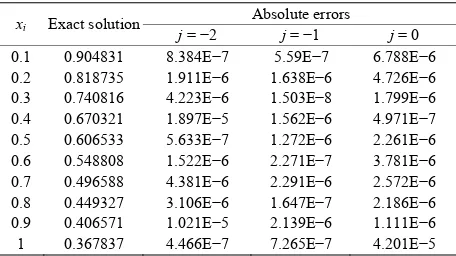
Consider the integral Equatio

 

e e _,

 

_, _e 

2

x x

x t

f x k x t



 

  and the exact solution is The numerical results are presented in Table 1.

Example 2

Consider the integral Equation (1) with;

 

1 e ,x

 

, 1

f x    x  k x t   x t

exact solution is

andb = 1,and the

 

e x

y x x  . The presented in Table 2.

numerical results are

Example 3

 

sin ,

 

, cos





f x x x k x t  x t

tion is

and the exact

solu- 

2sin

y x  x. The nume sented in Table 3.

rical result are

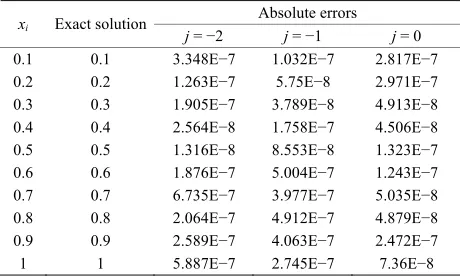
pre-Example 4

 

4

 

1 2

2 1

, , ,

3 3

g x  x x k x t k x t xt, and the exact solution is y x

 

x.

e 4.

The numerical results are presented in Tabl

[image:5.595.309.537.452.580.2]

Absolute errors

Table 1. The absolute errors for example 1.

xi Exact solution

[image:5.595.309.539.608.733.2]

j = −2 j = −1 j = 0 0.1 0.904831 8.384E−7 5.59E−7 6.788E−6 0.2 0.818735 1.911E−6 1.638E−6 4.726E−6 0.3 0.740816 4.223E−6 1.503E−8 1.799E−6 0.4 0.670321 1.897E−5 1.562E−6 4.971E−7 0.5 0.606533 5.633E−7 1.272E−6 2.261E−6 0.6 0.548808 1.522E−6 2.271E−7 3.781E−6 0.7 0.496588 4.381E−6 2.291E−6 2.572E−6 0.8 0.449327 3.106E−6 1.647E−7 2.186E−6 0.9 0.406571 1.021E−5 2.139E−6 1.111E−6 7 4.466E−7 7.265E−7 4.201E−5 1 0.36783

Absolute errors

xi Exact solution

j = −2 j = −1 j = 0 0.1 0.0904738 1.381E−5 1.28E−6 9.954E−6

0.2 0.163753 8.994E−6 1.488E−6

3 0.222242 1.052E−5 1.81

7.303E−6 0.

413E−5 2. 4.37E−6

.639E−5 1.42E−7 4.349E−6 066E−5 4.466E−7 3.997E−6 4.136E−6

0. 0.365915 3.425E−5 8.

1 0.367799 5.7E−6 1.

5E−6 3.265E−6

0.4 0.268129 5. 242E−6 1.059E−6

0.5 0.303268 1.689E−6 3.129E−6

0.6 0.329283 1

0.7 0.347614 1.

0.8 0.359459 5.727E−6 1.692E−6

9 073E−7 2.444E−6

094E−6 8.08E−5

(6)

209

Absolute errors

xi Exact solution

j = 0

j = −2 j = −1

0.1 0.0099833 8.384E−7 2.019E−6 4.092E−5 0.2 0.0397339 1.911E−6 6.551E−6 4.573E−5 0.3 0.0886561 4.223E−6 1.739E−7 1.081E−6

−5 2.08

2.535E−6 1.028E−6 047E−7 2.235E−6

0.7 E−5

0.8 0.573885 3.106E−6 4.201E−7 9.272E−6

1. −5 2.303E−5

0.4 0.155767 1.897E 2E−6 2.818E−5

0.5 0.239713 5.633E−7 0.6 0.338785 1.522E−6 8.

0.450952 4.381E−6 5.533E−6 1.412

0.9 0.704994 021E 662E−7 2.

3.581E−6

[image:6.595.57.287.100.242.2]

1 0.841471 4. 985E−6 3.251E−6

Table 4. The rro pl

A rs

absolute e rs for exam e 4.

bsolute erro

xi Exact solution

j = −2 j = −1 j = 0 0.1 0.1 3.348E−7 1.032E−7 2.817E−7

0.2 0.2 1.263E−7 5.75E−8 2.971E−7

0.3 0.3 1.905E−7 3.789E−8 4.913E−8 0.4

5 0. 0.4

5

2.564E−8 1.316E−

1.758E−7 8.553E−8 1.

4.506E−8 323E−7 0.

0.6 E−7

0.7 0. −8

2.064E−7 4.879E−8

8

0.6 1.876E−7 5.004E−7 1.243 7 6.735E−7 3.977E−7 5.035E

0.8 0.8 4.912E−7

0.9 0. 1

9 1

2.

5.887E−7

589E−7 4.063E−7 2.472E−7 7.36E−8 2.745E−7

In the ble the notation E h

d te nd j the R

7 on

Re

In this p hav a b d

V erra equa th nd,

d-holm-Volte integr pro r-

g e theo for rica n o a

integral eq ons an m- inte -

tions respectively. It e i to extend the

results to t en e f e d

equations a t ag m

R

N

[1] E. B. Lin and N ge let or

above ta s, we use − n whic e- no s 10n_a _denotes _{level of M A.}

. C

cluding

mark

aper we e shown etter metho in solving olt integral tions of e first ki and Fre

rra al equations. We also ve conve enc rem the nume l solutio f Volterr

uati d Frehol Volterra gral equa would b nteresting

wo-dim sional cas or the abov mentione nd apply o some im ing proble s.

EFERE CES

. Liu, “ eL ndre Wave Method f Numerical Solutions of Partial Differential Equations,”

Numerical Methods of Partial Differential Equation,Vol. 26, No. 1, 2010, pp.81-94. doi:10.1002/num.20417

,” Academic [2] C. K. Chui, “In Introduction to Wavelets

Press, Boston, 1992.

[3] E. B. Lin and X. Zhou, “Coiflet Interpolation and Ap- proximate Solutions of Elliptic Partial Differential Equa- tions,” Methods for Partial Differential Equations, Vol. 13, No. 4, 1997, pp. 302-320.

[4] M. T. Rashad, “Numerical Solution of the Integral Equa- tions of the First Kind,” Applied Mathematics and Com- putation, Vol. 145, No. 2-3, 2003, pp. 413-420.

doi:10.1016/S0096-3003(02)00497-6

[5] A. S. Shamloo, S. Shaker and A. Madadi, “Numerical Solution of Fredholm-Volterra Integral Equation by the Sunc Function omputation Mathe- matics, Vol. 2 2.

,” American Journal C

, No. 2, 2012, pp. 136-14

[image:6.595.57.287.267.405.2]