Permeability and kinetic coefficients for mesoscale BCF surface step dynamics: Discrete two- dimensional deposition-diffusion equation analysis

2016

Permeability and kinetic coefficients for mesoscale

BCF surface step dynamics: Discrete

two-dimensional deposition-diffusion equation analysis

Renjie Zhao

Iowa State University

James W. Evans

Iowa State University, [email protected]

Tiago J. Oliveira

Universidade Federal de Vicosa

Follow this and additional works at:

http://lib.dr.iastate.edu/physastro_pubs

Part of the

Condensed Matter Physics Commons

The complete bibliographic information for this item can be found athttp://lib.dr.iastate.edu/physastro_pubs/449. For information on how to cite this item, please visithttp://lib.dr.iastate.edu/howtocite.html.

Permeability and kinetic coefficients for mesoscale BCF surface step

dynamics: Discrete two-dimensional deposition-diffusion equation

analysis

Abstract

A discrete version of deposition-diffusion equations appropriate for description of step flow on a vicinal

surface is analyzed for a two-dimensional grid of adsorption sites representing the stepped surface and

explicitly incorporating kinks along the step edges. Model energetics and kinetics appropriately account for

binding of adatoms at steps and kinks, distinct terrace and edge diffusion rates, and possible additional

barriers for attachment to steps. Analysis of adatom attachment fluxes as well as limiting values of adatom

densities at step edges for nonuniform deposition scenarios allows determination of both permeability and

kinetic coefficients. Behavior of these quantities is assessed as a function of key system parameters including

kink density, step attachment barriers, and the step edge diffusion rate.

Disciplines

Condensed Matter Physics | Physics

Comments

This article is published as Zhao, Renjie, James W. Evans, and Tiago J. Oliveira. "Permeability and kinetic

coefficients for mesoscale BCF surface step dynamics: Discrete two-dimensional deposition-diffusion

equation analysis."

Physical Review B

93, no. 16 (2016): 165411, doi:10.1103/PhysRevB.93.165411. Posted

with permission.

Permeability and kinetic coefficients for mesoscale BCF surface step dynamics: Discrete

two-dimensional deposition-diffusion equation analysis

Renjie Zhao,1,2_{James W. Evans,}1,2,3,*_{and Tiago J. Oliveira}1,2,4

1_{Ames Laboratory, USDOE, Iowa State University, Ames, Iowa 50011, USA}

2_{Department of Physics and Astronomy, Iowa State University, Ames, Iowa 50011, USA}

3_{Department of Mathematics, Iowa State University, Ames, Iowa 50011, USA}

4_{Departamento de F´ısica, Universidade Federal de Vic¸osa, 36570-900, Vic¸osa, Minas Gerais, Brazil}

(Received 15 December 2015; revised manuscript received 15 March 2016; published 8 April 2016)

A discrete version of deposition-diffusion equations appropriate for description of step flow on a vicinal surface is analyzed for a two-dimensional grid of adsorption sites representing the stepped surface and explicitly incorporating kinks along the step edges. Model energetics and kinetics appropriately account for binding of adatoms at steps and kinks, distinct terrace and edge diffusion rates, and possible additional barriers for attachment to steps. Analysis of adatom attachment fluxes as well as limiting values of adatom densities at step edges for nonuniform deposition scenarios allows determination of both permeability and kinetic coefficients. Behavior of these quantities is assessed as a function of key system parameters including kink density, step attachment barriers, and the step edge diffusion rate.

DOI:10.1103/PhysRevB.93.165411

I. INTRODUCTION

In 1951, Burton, Cabrera, and Frank (BCF) introduced a strategy to describe the evolution of surface morphologies based upon coarse graining of an atomistic-level treatment [1]. This BCF formulation applies for crystalline surfaces or epitaxial thin films with a well-defined terrace-step structure and with characteristic lateral lengths on the mesoscale. It describes step edges by continuous curves and uses appropriate evolution laws to track their motion [2,3]. This approach can be applied to analyze step flow during deposition on vicinal surfaces; nucleation and growth of two-dimensional (2D) monolayer islands during deposition on flat surfaces where islands have a mesoscale lateral dimension due to facile sur-face diffusion; subsequent mound formation during unstable multilayer growth; and post-deposition island coarsening and mound decay [2,4,5].

The BCF prescription of step propagation is based on determination of fluxes of deposited atoms attaching to step edges. These fluxes in turn follow from analysis of the deposition-diffusion equations for the densities of diffusing adatoms on each of the terraces in a quasi-steady-state regime after imposing suitable boundary conditions (BC) at the step edges [1,2]. The original Dirichlet BC implemented by BCF treated steps as perfect traps for diffusing adatoms at which their density adopts its equilibrium value. This prescription was extended in 1961 by Chernov to incorporate possible inhibition in attachment of diffusing adatoms to steps, as characterized by kinetic coefficients K_± for ascending (+) and descending (−) steps [6]. LowerKvalues correspond to greater inhibition, soKmeasures the ease of attachment. There exist extensive analyses of step dynamics in both the diffusion-limited regime with highK, and the attachment-limited regime with lowK[2,3].

In 1992, Ozdemir and Zangwill introduced the concept of step permeability or step transparency associated with

*_{Corresponding author: [email protected]}

direct transport across steps between terraces (without in-corporation), the propensity for which is characterized by a permeabilityP[7]. ForP>0, deposition-diffusion equations on different terraces are coupled. Previous BCF type analyses incorporating step permeability have explored the transition to step flow [8] and step bunching or step instability on vicinal surfaces [3,9–11] during deposition. Other studies have explored the effect of permeability on second-layer nucleation during deposition [12,13], and on mound slope selection during unstable multilayer film growth [14]. In addition, the influence of permeability on post-deposition mound decay has been analyzed [15]. Analysis of experimental data has indicated significant permeability on Si(100) surfaces [16], but not on Si(111) surfaces [17]. In this study, our focus is not in BCF analyses of morphological evolution incorporatingP, but rather on systematic derivation ofP(and of theK_±) from an atomistic-level model. Furthermore, we will elucidate the dependence ofPon key system parameters.

Next, we review theoretical formulations and analyses for K_± and P. Some understanding has traditionally come from a steady-state analysis of discrete one-dimensional (1D) deposition-diffusion equation (DDE) models with the caveat that these models cannot account for step structure [4,5,18]. The classic analysis in the absence of permeability quantifies the decrease in K with increasing strength of an additional barrier for attachment to steps [19]. Permeability has also been incorporated into these 1D DDE models, at least in a simplistic fashion [18,20]. We will refine this treatment, thereby obtaining additional insight into the form ofP. An important feature already apparent from these 1D analyses is the lack of a unique procedure to connect the discrete model to continuum formulation, and thereby to extract associatedK’s andP.

uniform deposition on a perfect vicinal surface with a single type of step having symmetric attachment barriers (or no barriers), permeability does not affect behavior (see Sec.II), and one can directly determine the singleK(but notP) [18]. However, if the single type of step has asymmetric attachment barriers, then one can obtain two relationships between the two distinctK_± andP, but one cannot separately determine these quantities. Thus, to avoid this deficiency and enable determination of both K’s and P, in the current study, we also explore behavior for nonuniform deposition on vicinal surfaces. Specifically, we allow different deposition rates on different terraces. Note that in the absence of the deposition on a specific terrace, a nonzero adatom density on that terrace can only develop due to step permeability. Just as for the discrete 1D DDE approach, there will be some nonuniqueness in the definition and extraction ofK_±andPfrom this formalism.

For comparison with our analysis based on discrete 2D DDE, it is appropriate to remark on other strategies for assessingP(andK_±) incorporating 2D surface geometries. A quite distinct approach is based on continuum models for step dynamics incorporating multiple density fields. Specifically, these approaches include separate density fields for edge and terrace adatoms, and also include additional information about step structure such as the mean kink density or even a kink density field [22–24]. Such analyses typically require some approximations, but they do provide expressions both for the kinetic coefficients, and for the step permeabilityP. The predicted behavior forK_±andPis intuitively reasonable. For example,Pshould decrease with increasing step attachment barrier, and with increasing step edge diffusivity allowing efficient transport to and incorporation at kink sites [22,23].

Lastly, we mention one targeted kinetic Monte Carlo simulation study of a stochastic lattice-gas model which assessed the propensity for step crossing as a function of step attachment barriers and kink separation [25]. Clearly this crossing propensity is closely related to permeability, and these simulations indicated a qualitative dependence on model parameters consistent with previous studies.

In Sec.IIwe review continuum and discrete DDE model formalisms, and present new results for a refined 1D DDE model. We present explicit results forK_±andPfrom extensive numerical analysis of the discrete 2D DDE for symmetric (or zero) attachment barriers in Sec.III, and for asymmetric attachment barriers in Sec. IV. Application of the results to specific systems is discussed, and conclusions are presented in Sec.V.

II. DISCRETE DEPOSITION-DIFFUSION EQUATION (DDE) FORMALISMS

First in Sec. II A, to provide further background on the BCF formulation, we briefly review the continuum BCF formulation. This formulation considers the adatom density per unit area ρ(x₋,t) at lateral position x₋=(x,y), where in our analysis steps on the vicinal surface will be aligned with thex direction. The kinetic coefficientsK_±for attachment to ascending (+) and descending (−) steps and the permeability

P appear in the boundary conditions to the continuum deposition-diffusion equations for ρ(x₋,t). The basic model

includes uniform deposition rate per unit area F. Refined models will include different deposition rates Ft1 and Ft2

on alternating terraces. Another key parameter is the terrace diffusion coefficientD.

Next, we review discrete 1D DDE formulation in Secs.II B

andII C, and the 2D DDE formulation in Secs. II D and II E, as well as the procedure for obtaining K_± andP. The 1D formulation will correspond to a reduced version of the 2D formulation. Thus here we highlight some basic features of the discrete 2D DDE formulation. Adatoms reside at a square array of adsorption sites labeled (i,j) with lattice constanta

and with steps on the vicinal surface aligned with theiaxis. The adatom density at these sites is denoted byn(i,j), leaving implicit thet dependence, and corresponds to the probability that site (i,j) is occupied. One hasn(i,j)1 under typical conditions. The basic model includes uniform deposition at rateFper site, and refined models include different ratesFt1

andFt2on alternating terraces. Terrace diffusion corresponds

to hopping to nearest-neighbor (NN) empty sites at ratehper direction. Diffusive dynamics at step edges differs from that on terraces, we comment on some key aspects below.

In general, we include possibly asymmetric step attachment barriers leading to reduced ratesh_±for hopping to a straight step edge relative to the terrace hop rateh. We will write

h_±=exp(−βδ_±)h, where δ_± denote additional attachment barriers, assuming a common prefactor for all hops. Here+(−) corresponds to attachment to ascending (descending) steps, and we setβ =1/(kBT) where Tis the surface temperature and kB is the Boltzmann’s constant. The extra barrier δ₊

to attach to a descending step is described as the Ehrlich-Schwoebel barrier. Processes occurring at the step edge such as detachment, edge diffusion, equilibration, or incorporation, will be described in more detail below.

In our discrete DDE models, we will also allow the possibility of anisotropic NN lateral interactions mimicking, e.g., a fcc(110) versus a fcc(100) surface. However, for simplicity, we will retain isotropic terrace diffusion. NN attractions in the direction orthogonal (parallel) to the step will have strengthφ_⊥>0 (φ_||>0). Consequently, step edge adatoms are bonded to the straight step by a NN attraction of strengthφ_⊥>0 orthogonal to the step, and the rates for detachment from straight steps are given by exp(−βφ_⊥)h_±

according to detailed balance. Adatoms at kink sites have an additional bond of strengthφ_||>0 parallel to the step, and thus a total bonding of φb=φ_⊥+φ_||. Naturally setting the density of atoms at kink sites asn(kink)=1, it follows that the equilibrium densities in the absence of deposition are

neq(edge)=exp(−βφ||)n(kink)=exp(−βφ||) (1)

and

neq(terrace)=exp(−βφ⊥)neq(edge)

=exp(−βφb)n(kink)

=exp(−βφb)≡neq, (2)

for step edge and terrace adatoms, respectively.

density. More specifically, the rescaled spatially continuous density fielda2ρ(x₋,t) should be regarded as passing smoothly through the discrete densities n(i,j). Thus, one has that the continuum equilibrium density satisfies ρ_eq=a−2_n

eq,

with neq defined by (2). Sometimes it will be instructive

to introduce “excess densities”δρ=ρ−ρeqor equivalently δn(i,j)=n(i, j)−neq. In this mapping between discrete and

continuous models, the deposition rate per unit area in the continuum model is given byF=a−2_{F, orF}

ti=a−2Fti, and

the terrace diffusion rate satisfiesD=a2_{h. Below we shall see}

that there is some ambiguity or flexibility in mapping discrete onto continuous models which result in slightly different expressions forK_± andP. Also, in the discrete model, there is potentially a significant contribution to step propagation velocity from adatoms depositing directly at the step edge (i.e., at the row of sites directly adjacent to the step edge) [21]. The precise form of this contribution is tied to the definition ofK_±. Such a contribution is clearly absent in the continuum formulation.

A. Review of continuum BCF formulation

The traditional continuum BCF formulation considers uniform deposition where again F denotes the deposition flux per unit area, andDis the terrace diffusion coefficient. One performs a quasi-steady-state analysis of the continuum deposition-diffusion equation for the adatom densityρ(x₋,t) of the form

∂/∂t ρ(x₋, t)=F+D∇2ρ(x₋,t)≈0. (3)

General Chernov-type BCs at permeable step edges have the form

J_±= ±D∇nρ|±=JK±+JP,

where JK_±=K_±(ρ_±−ρeq) (4)

and JP =P(ρ_±−ρ_∓).

Here J_± denote the net diffusion fluxes for attachment to an ascending step from the terrace below (+), and to a descending step from the terrace above (−), respectively.

J_± incorporate two types of contributions.JK± denote those

associated with step attachment and detachment, whereK_±are the corresponding Chernov kinetic coefficients. JP denotes the contribution from step crossing, where P is the step permeability.∇ndenotes the gradient normal to the step.ρ_±are

the limiting values of the terrace adatom density approaching the step on the lower (+) and upper (−) terrace, respectively, andρeq denotes the equilibrium adatom density at the step.

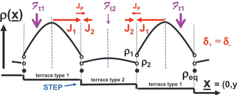
See Fig.1. It is common to setK_±=D/_±, where_±denote the attachment lengths, and P =D/p, where p denotes the permeability length. Then, large ’s implying difficult attachment or step crossing. The sign convention is chosen for a vicinal surface descending to the right and where we define net attachment fluxes to be positive,J_±>0.

Next, we discuss one example of behavior for a nonuniform deposition flux, specifically for flux switching between a larger valueFt1 and smaller valueFt2 on alternating terraces, and

where there is a symmetric attachment barrier so thatK₊= K₋=K. As illustrated in Fig.2, the density profile has mirror

STEP

(x)

0

<

<

-J

J

J

eq +

-

x

o o

FIG. 1. 1D schematic of adatom density and diffusion flux behavior at a step with asymmetric attachment. The total diffu-sion fluxesJ₊=K₊(ρ₊−ρeq)+P(ρ+−ρ−) andJ−=K−(ρ−− ρeq)+P(ρ−−ρ+) reaching the ascending and descending steps, respectively, and the flux across the step due to permeabilityJp=

P(ρ₋−ρ₊) are indicated.

symmetry about the center of each terrace, so the attachment flux has the same value on both sides of each terrace. We can readily extract some basic information about the density profile by balancing deposition and attachment fluxes on each terrace, i.e.,Ji =1/2FtiW. Letρidenote the adatom density at

the edge of terracei=1 or 2, andδρi =ρi−ρeqdenote the

corresponding excess density. Then, by adding and subtracting the expressions forJ1andJ2and rearranging the results, we

obtain the following relations:

δρ1−δρ2 =1/2(Ft1−Ft2)W/(K+2P)

(5) and δρ1+δρ2 =1/2(Ft1+Ft2)W/K.

A particularly instructive case is whenFt2=0, so then the

adatom density is uniform on terrace 2, and the associated excess density satisfies

δρ₂=1_/2WFt

1P /[K(K+2P)]. (6)

Thus, the excess density on terrace 2 in the absence of deposition is only nonzero ifP>0, and its magnitude provides a measure ofP.

B. Discrete 1D DDE model: Basic formulation

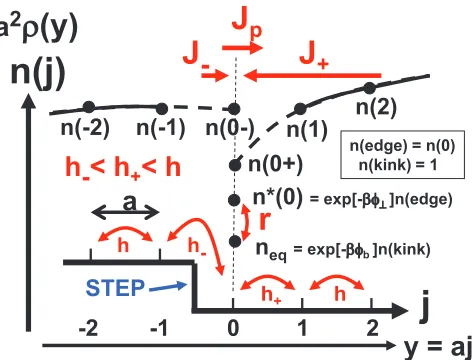
For a vicinal surface with straight parallel steps aligned with theiaxis (i.e., thexdirection), the simplest picture anticipates that the adatom density is independent of position along the step, but varies across the terrace. Thus,n(i,j)=n(j) depends

STEP

(x)

+ =

-J₁ J₂

eq 2

1

x

o

o o o

o o o o

J₂ J₁

t2

t1 t1

terrace type 1

terrace type 1 terrace type 2

JP JP

-2 -1 0 1 2

n(0+)

n(1)

n(2)

h₊ h

STEP

n(j)

h

_-

< h

< h

n(-2) n(-1) n(0-)

h h

-J

_-

J

₊

J

_p

r

n*(0)

j

y = aj

a

2

(y)

a

n

= exp[-

n(edge) = n(0) n(kink) = 1

FIG. 3. Schematic of our discrete 1D DDE model.n(j) denotes the adatom density on row j of sites, where j=0 corresponds to the step edge. Note that step detachment contributions are

d/dt n(±1)|detach=exp(−βφ⊥)h±n(0)=h±n∗(0). Note that n∗(0) coincides withn(0+) [n(0−)] in the case of zero attachment barrier

δ₊[δ₋].

only on the labeljof the rows of sites parallel to the step and, equivalently, ρ(x₋,t)=ρ(y,t) in the continuum formulation. This feature reduces the discrete 2D DDE formulation to a discrete 1D DDE formulation. The specific form of the discrete 1D DDE for the adatom density at rows of sites away from the step edges is

d/dt n(j)=F +h jn(j),

(7) where jn(j)=n(j+1)−2n(j)+n(j−1),

where againhis the terrace hop rate. Separate equations are needed for the adatom density at or adjacent to steps, where the rates for hopping might be impacted by step attachment barriers, and by distinct processes at the step edge. See AppendixA.

A detailed schematic of behavior in our discrete 1D DDE model is provided in Fig. 3. In this prescription, n(j =

0) denote the densities of terrace adatoms, and n(j =0) denotes the density of step edge adatoms. As indicated in the introduction to Sec.II, our model includes reduced attachment rates h_± for hopping to the step edge (j =0) relative to h, and detachment rates exp(−βφ_⊥)h_± reflecting bonding of edge adatoms to the step with attractionφ_⊥. In addition, our model incorporates the feature that adatoms which hop to the step edge are not immediately incorporated into the growing crystal. This, in turn, reflects the feature that in realistic 2D models, adatom incorporation effectively only occurs at kink sites which can be rare on close-packed steps. The rate of incorporation or equilibration in our 1D model is denoted by an additional parameterνdefined through the relation

d/dt n(0)|relax= −ν[n(0)−neq(0)]. (8)

Below we will introduce a naturally rescaled relaxation rate

rand relaterandνto permeability. We note that our model is

similar in spirit, but different in detail from a model of Zhao

et al.[20].

Given the feature that our discrete 1D DDE model should mimic the more realistic 2D DDE model, the equilibrium edge adatom densityn_eq(0)=n_eq(edge) in the 1D model should be enhanced by a factor of exp(βφ_⊥) relative to the equilibrium terrace densityneq=exp(−βφb). Similar enhancement should

persist in the presence of deposition. This suggests that the edge atom density n(0)=n(edge) is naturally rescaled to

n∗(0)=n∗(edge)=exp(−βφ_⊥)n(0) making it comparable in magnitude to terrace densities. Using this notation, one has d/dt n(0)|relax= −r[n∗(0)−neq] with the rescaled rate r=exp(+βφ_⊥)ν.

C. Discrete 1D DDE model: Extraction ofK_±andP

Analysis involves obtaining expressions relating diffusion fluxes to the step edgeJ_± and adatom densitiesat the step edgesρ_±and from these extractK_±andP. However, there is some flexibility in the identification of bothJ_±andρ_±. The 1D DDE diffusion fluxes are most naturally identified from sites

j = ±1 to the step edge. Significantly, results depend upon the identification ofρ_±. These could most simply be taken as the densities a−2n(±1), at sites adjacent to the step site j =0 (labeled as the “nonextrapolation” case N). Alternatively, they can be chosen asa−2_{n(0±), where n(0±) are obtained}

by suitably “analytically extending” terrace adatom densities

n(j) to the site j =0 (labeled as case E for “extrapolate” or “extend”). We also note the nontrivial result for uniform deposition that the rescaled density at the step edge n∗(0) corresponds to the extrapolated densityn(0+) [n(0−)] in the case of no additional attachment barrier δ₊[δ₋]. Different choices produce slightly different results forK_± andP. We note that the same applies for other formulations which are also possible, e.g., determining the fluxes between sitesj = ±2 and

j = ±1, a choice denoted byM. See AppendixAfor further discussion.

Here we just report the results of the above analysis for cases

NandE. For caseN, whereρ_±are identified asa−2_{n(±1), one}

obtains

K_±(N)=arh_±/(h₊+h₋+r),

(9) so _±(N)=ah(h₊+h₋+r)/(rh_±)

and

P(N)=ah₊h₋/(h₊+h₋+r),

(10) so p(N)=ah(h++h−+r)/(h+h−).

For the caseE, whereρ_± are identified as the analytically extendeda−2n(±0), one obtains

K_±(E)=ar(h/h_±−1)−1/[(h/h₊−1)−1

+(h/h₋−1)−1+(r/ h)] (11) and

P(E)=ah(h/h₊−1)−1(h/h₋−1)−1/[(h/h₊−1)−1

+(h/h₋−1)−1+(r/ h)], (12) from which one can obtain corresponding expressions for

Next, we discuss behavior in key limiting regimes, and also compare results of theEandNtreatments. In the limit of instantaneous incorporation or equilibration at step edges

r→ ∞, one obtains K_±(N)→ah_± so _±(N)→ah/h_±, and K_±(E)→ah/(h/h_±−1) so _±(E)→a(h/h_±−1). One also naturally obtains P(N) → 0, so p(N)→ ∞, and P(E)→0, so p(E)→ ∞. In the limit of vanishing attachment barriers h₊=h₋→h, one obtains _±(N)→

a(2+r/ h)/(r/ h) andp(N)→a(2+r/ h), versus_±(E)∼ 2a/(r/ h) andp(E)→0. Thus, for generalh±=h, we find

that values of _±(N) and _±(E) differing by a as r→ ∞. Similarly, forh_±=h, we find that_±(N)→abut_±(E)→ 0, asr/h→ ∞. In both cases, values of_±(N) and_±(E), or difference between them, are far below the terrace width

W, and so solution of the appropriate boundary value problem continuum deposition-diffusion equations will produce similar behavior. Finally, we note that in the regime of strong inhibition of attachment to stepsh_±horβδ_±1, expressions from both formulations agree and reduce toK_±≈ahexp(−βδ_±) andP ≈ahexp(−βδ₊−βδ₋)/(r/ h).

We note some similarity between the forms in (11) and (12), and the corresponding expressions in Zhao et al. [20] who also applied a discrete 1D DDE approach which incorporated extrapolation of terrace densities to step edges. In particular, the combinations (h/h_±−1) naturally appear as a result of analytic extension or extrapolation. However, Zhao et al.

introduce a probability p_inc for incorporation of any atom reaching a step. There is not a simple mapping betweenrand

pinc, although one haspinc→1 (0), asr/ h→ ∞(0) [26]. It is

also appropriate to note that (9) and (10) match the correspond-ing expressions obtained by Pierre-Louis [22] from a quite different continuum approach with multiple diffusion fields.

An additional question of particular relevance is how ν

or r, and thus P andK’s, are related to additional physical parameters in a realistic 2D model, such as the edge diffusion rate and kink density. Such parameters do not appear explicitly in our 1D model. Consider systems with facile edge diffusion associated with hop ratehe> h, and steps with a mean kink

separation Lk=lka. Then, the characteristic time for edge diffusion mediated incorporation of a mobile edge atom at a kink should scale like τ ∼(lk)2_{/he based on the Einstein}

diffusion relation. The relaxation rateνshould then be given byν=1/τ so thatr∼exp(+βφ_⊥)he/(lk)2. This form forν

was suggested previously in Ref. [22]. It produces the scaling

K_±∼(ah)/(lk)2, aslk→ ∞. Note this latter scaling applies more generally than in the case of facile edge diffusion as demonstrated previously from analysis of the discrete 2D DDE for symmetric attachment barriersh₊=h₋[21].

Finally, we mention that conventional versions of discrete 1D DDE models set r= ∞corresponding to instantaneous equilibration or incorporation at the step edge [4,5]. Then, permeability can still be incorporated (somewhat artificially) by modifying the model to introduce direct hopping across steps, e.g., between sites j =1 and j = −1 at rate hp. See

AppendixAfor the associatedK_±andP.

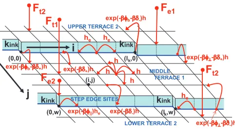
D. Discrete 2D DDE model: Formulation, definition ofK_±andP

Figure4shows a schematic of our discrete 2D DDE model. We consider a perfect vicinal surface with straight parallel

kink kink

kink kink

(0,0) (lk,0)

(0,w) (lk,w)

j

i

h h h

h

exp(- - +)h

exp(- - -)h

exp(- b- -)h

exp(- ||)he

exp(- +)h

exp(- -)h

exp(- b- +)h

STEP EDGE SITES

F

(i,j)

UPPER TERRACE 2

LOWER TERRACE 2 MIDDLE TERRACE 1

he he

he

F

F

F

F

FIG. 4. Schematic of our discrete 2D DDE model, indicating the rates for various hopping processes and depositions. Solution of the DDE equations just require analysis of densities in a periodic unit cell of sites, 0i < lk and 0j <2w. The unit cell consists of a strip between adjacent kink sites spanning two adjacent terraces.

steps aligned with thei direction and separated by terraces of equal widthW =w a (for integer w). We identify rows

j =0, j = ±w, j = ±2w, etc., as step edge rows, and rows

0j < w,wj <2w, etc. as being on the same terrace.

The vicinal surface descends with increasing j. Kink sites are specified to be periodically distributed along step edge rows with separationLk=lka, so kinks are located at (i,j)=

(nlk, mw) for integernandm. Thus, all steps are equivalent.

The discrete 2D DDE model accounts for variation of the adatom densityn(i,j) at site (i,j), both along the steps as well as across the terraces. Away from the step edges, the 2D DDE have the form

d/dt n(i,j)=F +h i,jn(i,j), (13)

where i,j is the discrete 2D Laplacian, so that i,j n(i, j)=n(i+1, j)+ n(i, j+1)+n(i−1, j)+n(i, j−1)− 4n(i,j). As discussed further below, refined equations are needed at and adjacent to step edges and at kink sites where the hop rates are modified reflecting possible attachment barriers at steps and binding at step edges. Kink sites constitute both a source and a sink for adatoms and the density of adatoms at kink sites is set to unity (as described above).

In our model with nearest-neighbor (NN) adatom attrac-tions, the interactionφ_||parallel to the steps controls the kink separation Lk≈1_/2aexp(1_{/2βφ||) [2]. Model behavior will}

depend onφ_|| only through kink separation as demonstrated in Ref. [18] by analysis of the discrete 2D DDEs for suitably rescaled adatom densities at step edges and kink sites. Model behavior also depends on the NN interactionφ_⊥ controlling edge adatom bonding to the step and the ratehefor diffusion along a straight step. Interestingly, from an analysis of rescaled 2D DDEs, it is possible to show that these parameters always appear in the combination exp(βφ_⊥)he/ h. Therefore, selecting

he=exp(−βφ⊥)h makes the model independent of φ⊥. In

some sense, the steps are “invisible” for this choice, since the effect of binding to the steps is compensated for by the effect of slower edge diffusion than terrace diffusion. We use this choice for most results presented in the following sections. In the general case with independentφ_⊥andhe, for isotropic

interactionsφ_||=φ_⊥as for fcc(100) homoepitaxy,Lkis tied

Ratesh_±for attachment to and detachment from straight steps have been described in the introduction to Sec.II. For completeness, we note that while direct attachment to kinks from terraces occurs at rate h_±=exp(−βδ_±)h, detachment from kinks directly to terraces occurs at rate exp(−βφ_⊥− βφ_||−βδ_±)h. Also, direct attachment of an edge adatom to a kink occurs at ratehe (as we do not include a separate kink attachment barrier along steps), and detachment from the kink to an edge site occurs at rate exp(−βφ_||)he. See Refs. [18,21] for further discussion.

For schematics of the 2D steady-state density profiles

n(i, j) from solving the 2D DDE, we refer the reader to Refs. [18,21]. Naturally these tend to have a global maxima in the center of the terraces furthest away from the kink sites which act as sinks for the excess adatom density. Along the step edge, the excess adatom density has maximum in between kink sites, i.e., δn(i,0)=n(i,0)−neq>0 is maximized in

between kink sites.

For extraction of K_± and P, our strategy is again to make a connection with the quasi-1D continuum formulation of Sec. II A. To this end, it is appropriate to consider the average along the step of the density profile n(i,j) in the discrete 2D DDE model. This average operation has the form

n(j) =(1/lk)₀i<lkn(i,j). In perhaps the most natural

formulation, one also calculates the average fluxesJ₊from rowj =1 to the stepj =0, andJ₋ from rowj = −1 to the stepj =0. Adatom densities at the step edgen_± can be identified with eithern(±1)or they can be obtained by extrapolating terrace densities to the step edges denoted by

n(0±). The former is the nonextrapolation case N in the notation of Sec.II B, and the latter is the extrapolation case

E. Then, for a uniform deposition fluxF, the K_± andPare defined to satisfy

J_± =a−2K_±(n_± −neq)+a−2P(n± − n∓). (14)

Since bothJ_± and averaged densities are directly pro-portional to F, the K_± and P are independent of F. We should emphasize that there is additional flexibility in the identification ofJ₊. An alternative to the above prescription might determineJ₊from the average flux from rowj =2 toj =1, andJ₋from rowj = −2 toj = −1. This choice, together with the identification ofn_± as n(±1), will be denoted byMfor modified flux choice. See also AppendixA

for a discussion for the corresponding 1D DDE models. Finally, we note that for the 2D DDE model, we can directly calculate the adatom density at the step edge, and thus extract the averaged quantityn(0). As in the discussion of the 1D DDE, we claim that it is natural to consider the rescaled version of this density n∗(0) =exp(−βφ_⊥)n(0) for comparison with adatom densities on the terrace. Of particular relevance for the analysis in Secs. III A–III C for uniform deposition is the nontrivial result that the rescaled density at the step edge n∗(0) corresponds to the extrapolated density

n(0+)[n(0−)] in the case of no additional attachment barrierδ₊[δ₋]. This behavior is analogous to that discussed for the 1D DDE.

E. Discrete 2D DDE model: Extraction ofK_±andP

Once the averaged fluxesJ_±and the averaged densities

n_± are determined from analysis of the 2D DDE model,

(14) for uniform deposition only yields two relations for three quantities. Consequently,K_±andPcannot be uniquely determined in this way. One exception to this scenario is when the steps have symmetric attachment barriers (or no attachment barriers), and as a consequence one has n₊ = n₋ so the permeability term is absent in (14). Then J₊ = J₋

and K=K₊=K₋ is determined from the single relation (14) which becomes J_± =a−2_Kδn

±, but here Pis still

undetermined [18]. Another exception is when just h₊=0 sinceδ₊= ∞ (infinite Ehrlich-Schwoebel barrier) and thus

K₊=0 (or just h₋=0 since δ₋= ∞ so K₋ =0). Now

P =0 and again (14) reduces to a single relation for a single nonzeroK[18].

To determine the individualK_± andPin the general case, and also to determinePfor symmetric barriers, an alternative analysis is required. To this end we consider situations with nonuniform deposition. A default choice is to select different deposition rates Fti, fori=1 or 2, on alternating terraces. More precisely, the rateFt1(Ft2) will apply for nonstep edge

sites nw < j <(n+1)w for even (odd) n. For step edge rows, it is convenient to have the flexibility to separately specify deposition ratesFei, fori=1 or 2, whereFe1 (Fe2)

applies forj =nwwith even (odd)n. One could setFe1=Ft1

andFe2=Ft2 corresponding to uniform deposition on each

terrace. See AppendixB. However, it will be more convenient to setFe1=Fe2=Ft1(orFt2) as this choice ensures symmetry

of the density profiles for symmetric attachment barriers (as discussed further below).

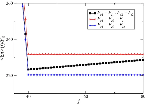
The feature that nonuniform deposition provides a natural vehicle to assess permeability is best illustrated by considering the special case for the “extreme” choice with no deposition on type 2 terraces, soFt1=F andFt2=0. With symmetric

attachment barriers described by a singleK, the excess density on type 2 terraces is uniform by symmetry, and should adopt the value

δn2=n2−neq≈1/2W F P /[K(K+2P)], (15)

based on the continuum analysis (6). Thus, δn₂ only has significant nonzero values in the presence of permeability

P > 0. Asymmetric attachment barriers produce a more complicated scenario given the linear variation in adatom density across the type 2 terrace. See Sec.IV.

Naturally, density profiles for any choice of Ft1=Ft2

will incorporate information on P. For the general case of

Ft1> Ft2, we now describe the strategy to extract K’s and

P, but also comment on additional perhaps unanticipated complications with this analysis. In general, there is distinct behavior at ascending and descending steps on each terrace. We initially assign distinct kinetic coefficientsK1± (K2±) for

the type 1 (type 2) terrace, where physically one would expect thatK1+ =K2+ andK1−=K2−since there is only a single

type of step in the model. Behavior of fluxes and densities at the step edges give four relations determining these K’s in terms of P. We can for example use these relations to obtainK1±=K1±(P) andK2±=K2±(P) as functions of an

unknownP. We can then demand that theK₊agree on both terraces, i.e.,K1+(P)=K2+(P) yieldingP =P+. However,

from this analysis would be consistent with the relationships determined from the density profiles. However, whileP₊and

P₋are generally close, they are not exactly equal.

We emphasize, however, that it is not reasonable to expect that unique consistent K_± andP can be extracted from the discrete 2D DDE model for arbitrary choices of parameters. Such 2D atomistic-level models cannot be exactly described within a 1D continuum formalism. Even in simple cases where

Pis not relevant,K_±values depend upon the interpretation of the adatom density at step edges. In contrast to the traditional continuum picture, we also know thatK_±depend on numerous details of the system such as terrace widths and in fact on the entire terrace distribution [18].

One exception avoiding the above inconsistency is the case with symmetric attachment barriers and where

Fe1=Fe2=Ft1 or Ft2. Then, by symmetry of the adatom

profile about the center of the terraces, one has that

K1+(P)=K1−(P) andK2+(P)=K2−(P) and consequently

thatP =P₊=P₋is uniquely determined. Notwithstanding, we still find slightly different values ofK’s andPdepending on whether we select Fe1=Fe2=Ft1 or Fe1=Fe2=Ft2.

However, one can argue that it is most appropriate to utilize limiting values as Ft2/Ft1→1 corresponding to physical

uniform deposition where the discrepancy disappears. In the asymmetric case, a slight difference persists in K’s and P’s even after taking this limit.

III. PERMEABILITY AND KINETIC COEFFICIENTS FOR SYMMETRIC ATTACHMENT

In this case, one has that K₊=K₋=K. Our goal is to determine not just this single K, but also P. Again, we use E [N] to denote the case where ρ_± are interpreted as the extrapolated n(0±) [as the nonextrapolated n(±1)], and where fluxes J_± are from rows j = ±1 to the step edge. M denotes a modified treatment whereJ_± are from rowsj = ±2 toj = ±1 and ρ_± are interpreted as n(±1). Various simple relationships betweenK_± for these different formulations are described in AppendixC. Again, for uniform deposition, we recall thatK=a2_J

±/δn±, whereJ+ =

J₋andδn₊ = δn₋.

A. Basic behavior for zero attachment barriers

Our default analysis will involve steps with substantial kink separationLk=24a corresponding toβφ_||=7.66. We also setφ_⊥=φ_||and choose “slow” edge diffusion with rate

he=exp(−βφ⊥)h(so that results are independent ofφ⊥) and

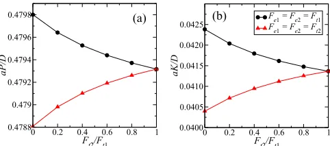
terrace widthW=40a. We consider deposition with differing ratesFt1 > Ft2 on alternating terraces. For the extreme case

of Ft2=0, the averaged adatom density profile is shown in

Fig.5, and one obtains for the nonextrapolation approach (in units ofah)

P(N)=0.479 80 (or 0.478 81)

(16) and K(N)=0.040 40 (or 0.042 38),

setting step edge deposition rates as Fe1=Fe2= Ft1(orFe1=Fe2=Ft2). The high value ofPand low value

ofK(despite the lack of step attachment barriers) reflects the large kink separation which inhibits incorporation at kink sites.

0 20 40 60 80

j

200 300 400

<

δ

n>

(

j

)

/F

t1

F_e1 = F_e2 = F_t1 F

e1 = Fe2 = Ft2

JK₁₋=K<δn1−>

JP=P(<δn1−> − <δn2+>)

JK1+=K<δn1+>

JP JK2−=K<δn2−>

JK2+=K<δn2+>

JP

JP=P(<δn1−> − <δn2+>)

JP=P(<δn1−> − <δn2+>)

JP

FIG. 5. Average adatom density profileδnrescaled by fluxFt1 as a function of terrace positionj. Data forh=1, W =40a, Lk= 24a, δ₋=δ₊=0 and deposition fluxes Ft1>0 andFt2=0. The arrows pointing right (left) indicate the diffusive fluxes for descending (ascending) steps, atj=0, 40, and 80. These show the cancellation of flux on the right terrace 2.

The discrepancy in values ofPandKfor different choices of edge deposition is eliminated by considering behavior as

Ft2/Ft1→1, as shown in Fig. 6. This yields the unique

limiting valuesP(N)=0.479 32 andK(N)=0.041 37, dif-fering only slightly from the values forFt2/Ft1=0. A similar

scenario applies using the modified (M) approach where distinct limiting values of P(M)=0.454 74 and K(M)= 0.039 25 are found. Significantly, all of these limiting K_±

equal the ones found in a standard analysis [18] for uniform deposition (Fe1=Fe2=Ft2=Ft1), from whichPcannot be

determined, so our methods to extract theK_±are consistent. For the extrapolation (E) approach, one finds thatK(E)= 0.043 15 andP(E)= ∞, the latter result reflecting the feature thatn(0+) = n(0−), so thatρ₊=ρ₋and any discrepancy between J_± and JK_± forces infinite P. The feature that

P = ∞might also be anticipated from our discrete 1D DDE

0 0.2 0.4 0.6 0.8 1 F_t2/F_t1

0.0400 0.0405 0.0410 0.0415 0.0420 0.0425

aK/D

F_e1 = F_e2 = F_t1 F_e1 = F_e2 = F_t2

(b)

0 0.2 0.4 0.6 0.8 1 F_t2/F_t1

0.4788 0.479 0.4792 0.4794 0.4796 0.4798

aP/D

(a)

10 20 30 40 50 60 L_k/a

0.4 0.42 0.44 0.46 0.48 0.5

aP/D

M N

0 10 20 30 40 50 60

L_k/a

0.014 0.015 0.016 0.017

a

(Δ

P

)

/D

(a)

0 10 20 30 40 50 60

L

k/a 0.00

0.05 0.10 0.15 0.20

aK/D

M N E

0 10 20 30 40 50 60

L_k/a

0 0.01 0.02 0.03

a

[

K

(

E

)−

K

(

X

)]

/D

X = N X = M

(b)

FIG. 7. Variation of (a)P’s and (b)K’s (from different approachesM,N, andE) with the kink separationLk. The insets show the differences

P =P(N)−P(M), K(E)−K(N), andK(E)−K(M) versusLk. Data forW=60a, δ−=δ+=0, andFt2/Ft1→1.

analysis for case E in Sec. II C. Thus, in Secs. III B and

III Cfor zero attachment barrier, we do not report values for

infiniteP(E).

B. Dependence on kink separation for zero attachment barriers

Recalling the relationLk≈1/2aexp(1_{/2βφ||) [2] for kink}

separation, we adjustLkby adjustingβφ||. First, let us consider φ_⊥=φ_||, as in Sec.III A, retaining an edge diffusion ratehe=

exp(−βφ_⊥)hso that behavior is independent ofheandφ_⊥. In this analysis we set W =60a. From previous analyses with uniform deposition for zero or symmetric attachment barriers, it was shown that K naturally decreases with increasing kink separationLk [18]. Here we extend this analysis using

nonuniform deposition to also assess behavior ofP.

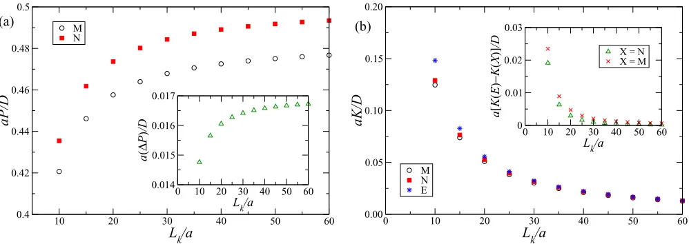
Results in the limit as Ft2/Ft1→1 for P and K versus Lk are shown in Fig.7. For casesNandM, one finds thatP

increases withLkbut saturates. Values depend on the choice of approach, the slight difference actually increasing withLk.

Presumably an expected increase ofPwith increasingLk is

counterbalanced by the effect of increasing φ_⊥ to produce saturation. We also find thatK ∼ah/(Lk/a)2, as Lk→ ∞, for any of the approaches N, M, or E [18]. This result can be understood from a rough analysis noting that J_± ≈ 1_/2a−2_{F W, and that the rescaled excess adatom density at the}

step edge follows from analysis of a 1D deposition-diffusion equation with adatoms impinging at rateJ_± and diffusing with hop ratehto sinks separated byLk. Thus, analysis of this 1D problem yields δn∗(0) = δn_±(E) ∼ J_±(Lk)2/(ah)

recovering the above form forK. Behavior ofδn_±(E)and

δn_±(N) should be similar in this case. A more complex semicontinuous version of this analysis can be found in an Appendix of Ref. [18]. The data shown in Fig.7 for smaller

Lkdoes not show pure asymptotic 1/(Lk)2_{scaling. However,}

behavior in this regime can be reasonably described by the more general form

K∼ah/[(Lk/a)2+B(Lk/a)+C]. (17)

The decrease inKwith increasingLkis certainly expected

as capture at far-separated steps is inhibited.

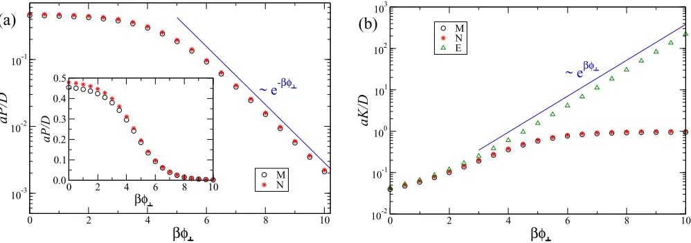
C. Dependence onheandβφ⊥for zero attachment barriers

As already noted, defininghe=exp(−βφ⊥)hmakesPand

Kindependent ofφ_⊥, since only the combination exp(βφ_⊥)he

appears in the rescaled 2D DDEs. However, in this section, we explore the more general case where he and φ_⊥ are regarded as independent parameters. For uniform deposition, behavior of K as a function of he can be assessed from

the relation K=a2_J

±/δn±. For this case where edge

diffusivity is decoupled from binding to the step edge, one expects that the rescaled excess adatom density right at the step edge satisfiesδn∗(0) ∼exp(−βφ_⊥)h/he(aJ_±/ h), for largehe/ horβφ_⊥. This result reflects the feature thatδn*(0) should scale inversely with he based on a simplified 1D

analysis. The first factor inδn*(0)reduces to unity for the choicehe=exp(−βφ_⊥)h, thus recovering standard results for that case. As noted above, for this case with zero attachment one has thatδn_±(E) = δn∗(0). This result, together with a relation in AppendixCallowing assessment of δn_±(N), yields

K(E)∼aheexp(βφ⊥)

(18) and K(N)∼aheexp(βφ_⊥)/[c+(he/ h)exp(βφ_⊥)],

forc=O(1) so thatK(N)∼ahfor largehe/ horβφ_⊥. This behavior is confirmed by results in Fig.8(b)for fixedφ_⊥and different ratioshe/ h, and also in Fig. 9(b) for varying φ_⊥

withhe=h kept constant. Clearly enhanced edge diffusion

enhances capture at kink sites resulting in higher values of

K. Enhanced binding at step edges also naturally produces enhanced adatom capture and enhancedK[provided thathe

does not decrease like exp(−βφ_⊥) asφ_⊥increases].

For the analysis of permeability (for the caseN) based on behavior for differing deposition fluxes on alternating terraces, it is perhaps simplest to consider the extreme case of no de-position on terrace 2. Then, the relation (15) together with the assumption thatP(N)K(N) andJ1 ≈1/2F W a−2 yields P(N)∼a−2_K(N)2_δn

2/J1. Then, using thatK(N)∼ah

for large he/ h or large βφ⊥, and the relation δn2 ∼

0 0.5 1 1.5 2 2.5 3 h

e / h 0

0.02 0.04 0.06 0.08 0.1

aP/D

M N

0 0.5 1 1.5 2 2.5 3

h_e / h

0 0.001 0.002 0.003 0.004

a

(Δ

P

)

/D

(a)

0 0.5 1 1.5 2 2.5 3

h_e / h 0.80

0.85 0.90 0.95

aK/D

M N

0 0.5 1 1.5 2 2.5 3

h_e / h

0 10 20 30 40 50 60 70

aK

(

E

)

/D

(b)

FIG. 8. Main plots: dependence of (a)P’s and (b)K’s (for approachesMandN) with the ratio of edge on terrace hopping rateshe/ h. Insets: (a) differenceP =P(N)−P(M) and (b)K(E) versushe/ h. Data forW=60a, Lk=30a, δ−=δ+=0, andFt2/Ft1→1.

forδn*(0)for uniform deposition, one concludes that

P(N)∼(ah) exp(−βφ_⊥)h/he, for large he/ horβφ⊥.

(19) See AppendixCfor an alternative analysis. The behavior predicted by (19) is confirmed in Figs.8(a)and9(a). Just as enhanced edge diffusion enhances capture at kinks, it also inhibits transport across steps (without capture). Likewise, enhanced binding at step edges naturally inhibits transport across steps.

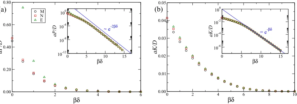
D. Nonzero symmetric attachment barriers

NowP(E) is finite, as well asP(N) andP(M), and we will see that these different formalisms produce similar behavior. In this case we chooseh_±=exp(−βδ)hand again sethe=

exp(−βφ_⊥)h. It is intuitively clear that bothK→0 andP→

0, asβδ→. Furthermore, for large attachment barriers, the adatom density on the terrace becomes more uniform including in the direction along the step. Thus, the discrete 1D DDE model should more accurately describe behavior in the 2D

model, and the prediction from (9) or (11) that

K_±≈ahexp(−βδ) (20)

should apply. Indeed, the results in Fig. 10 show that this behavior is realized for the 2D model after a crossover from a nonasymptotic regime for smallβδ. To elucidate the behavior ofP, again the discrete 1D DDE model provides insights noting that the relaxation rate describing incorporation of adatoms, which have already reached the step edge, will not decrease with increasingβδas such adatoms have already surmounted the step attachment barrier and just need to diffuse along the step edge to reach kink sites. Thus, the result from (10) and (12) that P ≈ah2_{exp(−2βδ)/r should be applicable. Even}

though a precise expression forris not available, this quantity will not depend onβδ. Results in Fig.10confirm the variation

P ∼ahexp(−2βδ). (21)

It is also appropriate to note that the behavior of K and

P is not sensitive to the detailed prescription (extrapolated, nonextrapolated, or modified) of these quantities.

0 2 4 6 8 10

βφ

10-3

10-2

10-1

aP/D

M N

0 2 4 6 8 10

βφ 0.0

0.1 0.2 0.3 0.4 0.5

aP/D

(a)

~ e-βφ

0 2 4 6 8 10

βφ

10-2

10-1

100

101

102

103

aK/D

M N E

(b)

~ eβφ

0 2 4 6

βδ

0.00 0.20 0.40 0.60 0.80

aP/D

M N E

0 5 10 15

βδ

10-12

10-8

10-4

100

aP/D

(a)

~ e-2βδ

0 2 4 6 8 10

βδ

0.00 0.01 0.02 0.03 0.04 0.05

aK/D

0 5 10 15

βδ

10-6

10-4

10-2

100

aK/D

(b)

= e-βδ

FIG. 10. (a) Permeability and (b) kinetic coefficient versus interactionβδ, withδ=δ₊=δ₋in linear (main plot) and log-linear (inset) scales. Data for different approaches forW=40a, Lk=24a, andFt2/Ft1→1 are shown.

IV. PERMEABILITY AND KINETIC COEFFICIENTS FOR ASYMMETRIC ATTACHMENT

Again in analyzingK’s andP, caseE[caseN] indicates that

ρ_± are obtained from extrapolatedn(±0) [nonextrapolated

n(±1)], and fluxesJ_±are from rowsj = ±1 to the step edge. M indicates that J_± are from j = ±2 to j = ±1 and ρ_± are interpreted as n(±1). Our default analysis will involve steps with substantial kink separationLk=24a

corresponding toβφ_||=7.66, he=exp(−βφ_⊥)h, and terrace widthW =40a.

0 20 40 60 80

j

200 300 400 500 600 700 800

<

δ

n>

(

j

)

/F

t

1

F_e1 = F_e2 = F_t1

F_e1 = F_e2 = F_t2

<

δ

n

>

<

δ

n

>

<

δ

n

>

<

δ

n

>

JK1− = Κ−<δn1−>

JP = P(<δn1−> − <δn2+>)

JP

JK1+ = Κ+<δn1+>

JP

JK2+ = Κ+<δn2+>

JK2− = Κ−<δn2−>

JP

FIG. 11. Average adatom density profileδnrescaled by flux

Ft1 as a function of terrace positionj, forh=1, W=40a, Lk= 24a, δ₊=0, δ₋=3.5, and deposition fluxes Ft1>0 andFt2=0. The arrows pointing right (left) indicate the diffusive fluxes for descending (ascending) steps, located atj=0, 40, and 80. Note that the flux is constant across the right terrace 2.

A. Basic behavior for nonzero ES barrier (δ−>0, δ+=0)

For the caseδ₋>0 [corresponding to a nonzero Ehrlich-Schwoebel (ES) barrier for downward transport at step edges] andδ₊=0 (facile attachment at ascending steps), it is clear

that K₋< K₊. We consider deposition with differing rates

Ft1> Ft2 on alternating terraces. For the extreme case of

nonuniform deposition with Ft2=0, the averaged adatom

density profile is shown in Fig. 11. Again the nonzero excess density of terrace 2 reflects the presence of a nonzero permeabilityP>0, and the linear variation across the terrace is a simple consequence of the lack of deposition which implies a constant diffusion flux across the terrace. Direction of the net flux across terrace 2 is perhaps not obvious as it is in the direction of the smaller of the two permeability fluxes impinging on terrace 2. This behavior also relies on the feature thatK₋ K₊.

Next, we present results forK_±andP’s based on an analysis as described in Sec.II Efor the limiting case of quasiuniform deposition (Ft2/Ft1→1). Specifically, after determining the

relations K1±(P) and K2±(P) from analysis of fluxes to

step edges and excess adatom densities on both terraces, we determineP₊andP₋from the relationsK₁₊(P₊)=K₂₊(P₊) andK1−(P−)=K2−(P−). For each of the approachesE,N,

andM, one finds small differences inP₊andP₋. See TableI

for some examples. For casesNandM,K₋is about 40% of

K₊ for βδ₋=0.8, and about 3% of K₊ for βδ₋=3.5. P

values are significantly higher thanK₊values forβδ₋=0.8, but about 50% lower for βδ₋=3.5. For case E, one finds somewhat higher values forK₊ andP, but extremely small values forK₋.

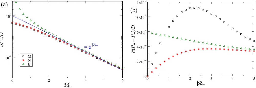
A more complete description of howP₊depends onβδ₋is given in Fig.12(a). As might be anticipated from our discrete 1D DDE analysis, one finds decay likeP_±∼(ah)exp(−βδ₋) for a broad range of largeβδ₋. The variation of the difference betweenP₊andP₋depends on the approachE,N, orM, but it is always very small and tends to decrease for largeβδ₋. See

Fig.12(b). Behavior ofP₊for very largeβδ₋has an unusual

TABLE I. PermeabilitiesP_±and kinetic coefficientsK_±=K1±(P±)=K2±(P±) for approachesM,N, andE. The slight difference between P₊andP₋is shown in the fifth column. Data are obtained forW=40a, Lk=24a, δ+=0, andFe1=Fe2=Ft1withFt2/Ft1→1.

βδ₋ Approach aP₊/D aP₋/D a(P₊−P₋)/D aK₊/D aK₋/D

0.8 M 0.279 54 0.278 98 0.000 56 0.048 13 0.021 55

N 0.294 46 0.294 26 0.000 20 0.050 66 0.022 76

E 0.816 51 0.815 97 0.000 55 0.077 36 0

3.5 M 0.026 81 0.026 07 0.000 75 0.053 03 0.001 20

N 0.028 05 0.027 69 0.000 36 0.055 10 0.001 66

E 0.031 55 0.031 14 0.000 41 0.060 10 0

K_±. As expected from the discrete 1D DDE analysis, one finds thatK₋∼(ah)exp(−βδ₋), whileK₊saturates for largeβδ₋. See Fig.13.

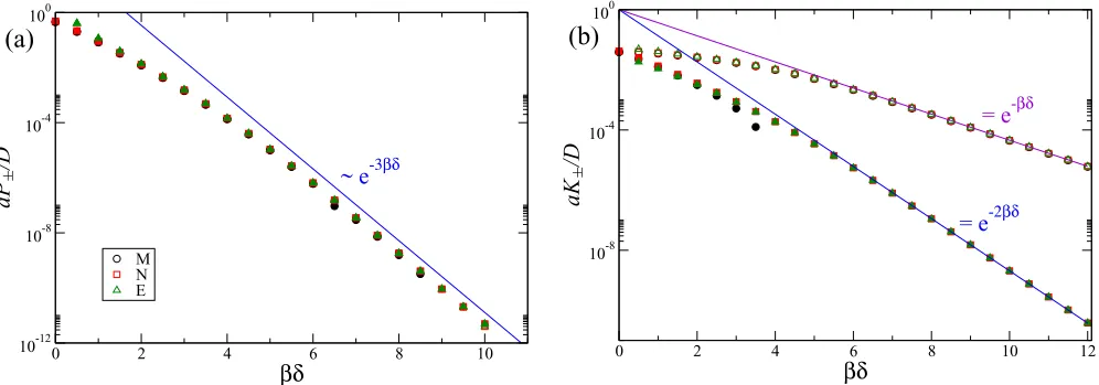
B. Behavior for asymmetric attachment barriers with δ−=2δ+=2δ

Again, as in Sec.III D, one expects that, for large barriers, the discrete 1D DDE model should more accurately describe behavior in the 2D model. Thus, (9) or (11) forK_± and (10) or (12) forPsuggest

K_± ≈ahexp(−βδ_±)

(22) and P ∼ahexp(−βδ₊−βδ₋)=ahexp(−3βδ).

Results shown in Fig.14confirm these predictions. Note that the behavior ofK andPis not sensitive to the detailed prescription (extrapolated, nonextrapolated, or modified) of these quantities.

V. DISCUSSION AND CONCLUSIONS

Our analysis shows that the discrete 2D DDE formulation is particularly effective at not just elucidating the general behavior of permeability Pand kinetic coefficients K_±, but also in quantifying these parameters. The latter is necessary for application to the description of specific systems where appropriate energetic and geometric parameters would provide input to our 2D DDE formulation. Steady-state analysis of

nonuniform deposition scenarios allows determination of each of Pand K_±. This is not possible just considering uniform deposition. For the extreme case where there is no deposition on alternating terraces, one gains immediate insight into the extent of permeability from the nonzero excess adatom density on those terraces.

To conclude, we review in more detail our results for the dependence ofPandK_±on key parameters, and also discuss how these results relate to behavior in specific systems:

(i) Dependence on kink separationLk. The behaviorK_± ∼ a3_h/(Lk)2 _{from (17) illustrating the decrease of K}

± with

increasingLk, which is expected since incorporation at kinks

is naturally inhibited. This dependence is key to understanding behavior during step flow on dimer-row reconstructed vicinal Si(100) or Ge(100) surfaces which exhibits alternating rough (or meandering) steps and smooth (or stiff steps) [18,21,27,28]. Rough (smooth) steps have low (high)Lkvalues, and thus high

(low)K_±values. Another class of systems are fcc(110) metal surfaces [29,30]. Here steps along the110direction (parallel to rows of neighboring surface atoms) are smooth and stiff with largeLk and lowK_±, but steps in the orthogonal001 direction are rough with lowLkand higherK±.

Dependence of P on Lk depends on model details. If

edge diffusivity decreases asLkincreases, thenPcan saturate as shown in Sec. III B. However, increasing Lk with other parameters fixed would naturally lead to a increase inP as suggested by (10) or (12) usingr∼exp(+βφ_⊥)he/(lk)2_.

0 2 4 6

βδ−

10-2

100

aP

+

/D

M N E

(a)

= e-βδ−

0 1 2 3 4 5

βδ−

0 2×10-4 4×10-4 6×10-4 8×10-4 1×10-3

a

(

P+

−

P−

)

/D

(b)