Predictability of Earthquake Occurrence Using Auto Regressive Integrated Moving Average (ARIMA) Model

(1)



Abstract—Earthquake, as a natural calamity, is devastating as it already killed eight hundred one thousand six hundred twenty-nine (801,629) people from years 2000 to 2017 all over the world. This study incorporated data mining techniques to find patterns about the occurrence of earthquake. The number of future occurrence of each magnitudes for the years 2018 to 2022 was forecasted using ARIMA(1,0,6) model. The simulation result shows that the highest count of earthquake occurrences is forecasted in year 2022 with estimated number of 1,580 times in magnitude level of 5.0-5.9. It only proved that the ARIMA(1,0,6) model is effective in predicting occurrences of earthquake. Future researchers may utilize other data mining techniques and conduct a comparative study on the different results.

Index Terms— arima, forecasting, prediction, earthquake, data analytics

I. INTRODUCTION

ATURAL risks [1] such as earthquakes, floods, hurricanes, tornadoes, tsunamis, volcanic eruptions and others are some of the threats in modern society. Among natural disasters, earthquake stands out due to their disturbing effects [2] as it also produces tsunamis [3], landslides [4] and soil liquefaction [5].

Analysis and processing of huge data has become a stronghold technique that is being applied in extracting useful information and discover patterns out of huge datasets [6]. In analyzing huge datasets, machine learning algorithms is required coined with new parallelized implementations to produce much better results [7].

With the abovementioned, global researches about earthquakes were conducted to intensify our understanding and have a grasp on the techniques to foresee them [8]. Various studies about earthquake predictability were conducted. Methods in data analytics such as random forest (RF) [9], artificial neural network (ANN), recurrent neural network, LPBoost [10] and other boosting methods, Naïve Bayesian, regression models, C4.5, KNN, linear regression [11], and SVM [12] has been utilized. In this paper, number

M

anuscript received December 21, 2018; revised January 30, 2019. T. L. Toledo is a student of Doctor in Information Technology at Cebu Institute of Technology, Philippines. She is currently connected at Surigao State College of Technology as an Associate Professor in the College of Engineering and Information Technology. (e-mail: [email protected]) C. J. Aliac. is a faculty and research coordinator of the Intelligent Systems Laboratory at CIT-University, Philippines. (e-mail: [email protected]).

of earthquake occurrences for the next five years is predicted.

II. MACHINE LEARNING TECHNIQUES FOR EARTHQUAKE

PREDICTION

It is believed that there is no such existing model capable of predicting earthquakes’ exact time, location and magnitude since its occurrence is random and due to high nonlinear phenomenon. Although, various studies over earthquake occurrences and predictions with the implementation of different algorithms has been already conducted which lead to various conclusions regarding the aspects under consideration [10].

A. Artificial Neural Network

The concept that lies behind the Artificial Neural Network are modeled based on the interconnected neurons in the human brain structure. A network is created with the combination of neurons that is made with individual nodes having represented by its own variables. The network consists of three layers vis., input, output, and hidden layers. This layer serves as a medium in providing connection between the input and output nodes. The result of the first initialization can be used as input to prior nodes to be processed. [13].

In training a network, back propagation algorithm is one supervised learning technique often used. Back propagation [14] method for forecasting are described in the following steps:

1) Assign a small pseudorandom value for a network weight W.

2) Using a sigmoid function F,

F(v) = tanh(v), (1)

compute the activation level Oj of the hidden and output

units.

3) Compute the error needs using the delta rule, E = ( – (2)

as represents the forecasted value while the actual value is being represented by within the output layer.

4) Compute the weights to update the network weights for all the weights from output layer to hidden layer,

Δ = η (3)

Predictability of Earthquake Occurrence Using

Auto Regressive Integrated Moving Average

(ARIMA) Model

Teresita L. Todelo, Chris Jordan G. Aliac

(2)

5) Redo steps 2 to 4 until the stopping criterion is has met.

B. Recurrent Neural Network

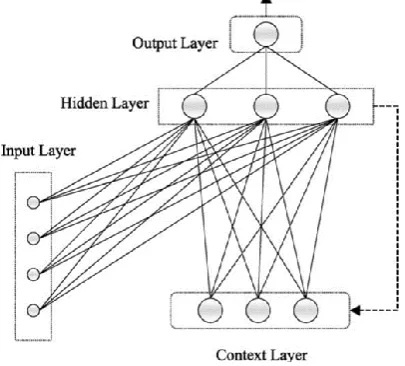
[image:2.595.66.269.213.396.2]

Fully recurrent networks [15], introduced by Elman, feed the outputs of the hidden layer back to itself. Partially recurrent networks start with a fully recurrent net and add a feedforward connection that bypasses the recurrence, effectively treating the recurrent part as a state memory. Fig. 1 depicts a typical recurrent network. It is being said that this method is a state of the art in nonlinear time series prediction, system identification, and temporal pattern classification [16].

Fig. 1. Typical recurrent neural network

C. Random Forest

The random forest (RF) is a technique of combining the prediction of many decision trees [17]. It refers to the large number of decision trees, merged through bootstrap aggregating or bagging. Bagging is the main principle where a sample of size n is randomly chosen from the training set and fitted to a regression tree. The said sample is known as bootstrap which is chosen with replacement.

In a taking bootstrap sample, each observation has the probability to be chosen at random. The random selection is represented by the random variables , independent and identically distributed. Using the bagging algorithm, several bootstrap samples ( ,…, ) were selected and applying the CART algorithm to them in order to obtain a collection of r predicting trees (f(X, ),…,f(X, )). The output of all these predictors are then aggregated.

D. LPBoost

Boosting is another method used to enhance the performance of weak learners such as in trees. Different boosting types varies based upon the weighting methodologies and LPBoost is one of these types. It is a linear combination of many tree classifiers. The idea is that each classifier is iteratively added to the set of selected classifiers until no other tree needs to be added [18].

E. Naïve Bayesian Classification

Naïve bayesian classifier is anchored on bayes theorem with a codition of independence between predictors. Bayes theorem gives a way on the calculation of the posterior probability, , from , and .Naive Bayes classifier has the assumption that the effect of a predictor (x) on a given class (a) is independent of other predictors. This assumption is called class conditional independence.

. .

where . . … . . .

(4)

is the posterior probability of class (target) given the predictor (attribute), is the prior probability of class, is the likelihood which is the probability of predictor [13].

F. KNN

The k-nearest neighbor algorithm is a powerful nonparametric classifier which assigns an unclassified pattern to the class represented by a majority of its k nearest neighbors. The KNN works as follows:

Find k nearest neighbors from the set T for the unknown query point x, and let ={( indicate the set of

k nearest neighbors for x. The distance between x and the neighbor is measured by the Euclidean distance metric

(5) The class label of the query point x is predicted by the majority voting of its neighbors

(6) where c is a class label and denotes the class label for the i-th nearest neighbor among its k nearest neighbors. The indicator function takes the value of one if the class of the neighbor is the same as the class c and zero otherwise [19].

G. Auto Regressive Integrated Moving Average

ARIMA model is considered one of the most widely used methodology in time series forecasting that aims to describe the autocorrelations in the data and use the ARIMA(p,d,q) notation. p denotes the order of auto regression process (AR), d refers to the degree of differentiation involved (I) and q refers to the (MA) which is the order of the Moving Average. The mathematical expression of the model is:

= + +…+ + - -

(3)

[image:3.595.304.552.47.383.2]

Fig. 2. Algorithms flowchart of ARIMA

III. EXPERIMENTS AND RESULTS

[image:3.595.53.288.61.227.2]

The data that were used in this study are the indexed datasets of earthquake counts around the world from years 2000-2017. This paper used ARIMA(1,0,6) model in determining the occurrence of earthquake for the next five years. The simulation was done using GRETL software application.

Fig. 3. Magnitude 5-5.9

[image:3.595.47.292.360.508.2]

Fig. 3 shows that there is a connivance with the actual and forecasted data. The forecasted data of magnitude 5-5.9 earthquake showed an increasing forecast from 2018 to 2022 with highest number of occurrence in year 2020 with 1,580 earthquakes all over the world. It is evident in the graph that the forecasted trend follows the pattern of the actual data and depicts a very close prediction like in the years 2014, 2006, and 2013 as compared in the simulation shown in Table I. The MAPE result shows that the forecasted data is 12% off from the actual data. Therefore, the forecast is reliable.

Table I. Comprehensive simulation result for magnitude 5-5.9

Year Actual

Data

Forecasted Data

Forecast evaluation

statistics Values

2000 1344 1585.51 Mean Error 5.033

2001 1224 1437.29 Mean Squared Error 62000

2002 1201 1365.92 RMSE 249

2003 1203 1363.23 MAE 205.1

2004 1515 1365.1 MPE -1.9535

2005 1693 1579.26 MAPE 12.795

2006 1712 1660.61 Theil's U 0.94047

2007 2074 1658.09 Bias proportion, UM 0.00040856

2008 1768 1907.47

Regression proportion, UR

0.0003116 6 2009 1896 1649.29 Disturbance proportion, UD 0.99928

2010 2209 1786.77

2011 2276 1975.64

2012 1401 1985.51

2013 1453 1382

2014 1574 1533.4

2015 1419 1587.58

2016 1550 1470.63

2017 1455 1583.11

2018 1496.24

2019 1541.23

2020 1563.55

2021 1574.62

2022 1580.11

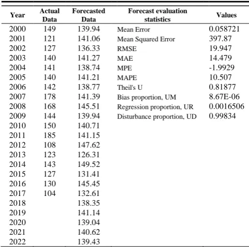
The forecasted data for magnitude 6-6.9 earthquake showed an increasing forecast from year 2017 to 2019 and an alternate decrease and increase on the succeeding years that is evident in Fig. 4. The MAPE result as shown in Table II depicts that the forecasted data is 10% off from the actual data. Therefore, the forecast is reliable.

Table II. Comprehensive simulation result for magnitude 6-6.9

Year Actual

Data

2000 149 139.94 Mean Error 0.058721

2001 121 141.06 Mean Squared Error 397.87

2002 127 136.33 RMSE 19.947

2003 140 141.27 MAE 14.479

2004 141 138.74 MPE -1.9929

2005 140 141.21 MAPE 10.507

2006 142 138.77 Theil's U 0.81877

2007 178 141.39 Bias proportion, UM 8.67E-06

2008 168 145.51 Regression proportion, UR 0.0016506 2009 144 139.94 Disturbance proportion, UD 0.99834

2010 150 140.71

2011 185 141.15

2012 108 147.62

2013 123 126.31

2014 143 149.52

2015 127 131.41

2016 130 145.45

2017 104 132.61

2018 138.35

2019 141.14

2020 139.04

2021 140.62

[image:3.595.308.552.519.761.2] [image:3.595.51.291.702.792.2]

(4)

[image:4.595.47.292.51.197.2]

[image:4.595.307.545.146.391.2]

The forecasted data for magnitude 7-7.9 earthquake showed an increased pattern from year 2008 to 2010 and an alternate decrease and increase on the following years up to year 2015. A successive decrease on the occurrence of earthquake having magnitude 7-7.9 is present in the year 2016 up to 2020 as evident in Fig. 5. The MAPE result as shown in Table III depicts that the forecasted data is 30% off from the actual data. Therefore, the forecast is reliable.

Table III. Comprehensive simulation for Magnitude 7-7.9

Year Actual

Data

2000 14 Mean Error 0.024002

2002 13 14.23 RMSE 4.6115

2003 14 13.14 MAE 3.5383

2004 14 13.23 MPE -9.8676

2005 10 13.53 MAPE 30.365

2006 9 10.74 Theil's U 0.94587

2010 23 14.33

2011 19 20.43

2012 12 19.74

2013 17 13.64

2014 11 15.03

2015 18 12.34

2016 16 15.43

2017 6 16.14

2018 8.54

2019 7.31

2020 7.21

2021 6.78

[image:4.595.55.550.313.783.2]

2022 6.44

Fig. 6. Magnitude 8 and up

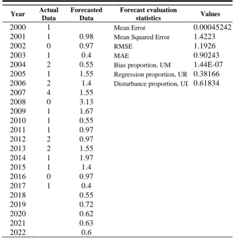
A steady pattern on the forecasted occurrence of earthquake having magnitude 8 and up in the year 2018 up to 2022 is evident in Fig. 6. The MAPE result as shown in Table IV depicts that the forecasted data is 30% off from the actual data. Therefore, the forecast is reliable.

Table IV. Comprehensive simulation result for magnitude 8 and up

Year Actual

Data

2000 1 Mean Error 0.00045242

2002 0 0.97 RMSE 1.1926

2003 1 0.4 MAE 0.90243

2007 4 1.55

2008 0 3.13

2009 1 1.67

2010 1 0.55

2011 1 0.97

2012 2 0.97

2013 2 1.55

2014 1 1.97

2015 1 1.4

2016 0 0.97

2017 1 0.4

2018 0.55

2019 0.72

2020 0.62

2021 0.63

2022 0.6

REFERENCES

[1] T. Aven, “On how to define, understand and describe risk,”

Reliab. Eng. Syst. Saf., vol. 95, no. 6, pp. 623–631, 2010.

[2] E. Florido, F. Martínez-Álvarez, A. Morales-Esteban, J. Reyes, and J. L. Aznarte-Mellado, “Detecting precursory patterns to enhance earthquake prediction in Chile,” Comput. Geosci., vol. 76, pp. 112–120, 2015.

[3] C. Cecioni, G. Bellotti, A. Romano, A. Abdolali, P. Sammarco, and L. Franco, “Tsunami early warning system based on real-time measurements of hydro-acoustic waves,” Procedia Eng., vol. 70, pp. 311–320, 2014.

[4] D. K. Keefer, “Geological Society of America Bulletin Landslides caused by earthquakes Landslides caused by earthquakes,” Geol. Soc. Am. Bull., vol. 95, no. 4, pp. 406–421, 1984.

[5] C. Clément, R. Toussaint, M. Stojanova, and E. Aharonov, “Sinking during earthquakes: Critical acceleration criteria control drained soil liquefaction,” Phys. Rev. E, vol. 97, no. 2, pp. 1–18, 2018.

[6] C. W. Tsai, C. F. Lai, H. C. Chao, and A. V. Vasilakos, “Big data analytics: a survey,” J. Big Data, vol. 2, no. 1, pp. 1–32, 2015.

[7] J. C. Jackson, V. Vijayakumar, M. A. Quadir, and C. Bharathi, “Survey on programming models and environments for cluster, cloud, and grid computing that defends big data,” Procedia

Comput. Sci., vol. 50, pp. 517–523, 2015.

[8] X. Romão, E. Paupério, and N. Pereira, “A framework for the simplified risk analysis of cultural heritage assets,” J. Cult.

Herit., vol. 20, pp. 696–708, 2016.

[9] B. Rouet-Leduc, C. Hulbert, N. Lubbers, K. Barros, C. J. Humphreys, and P. A. Johnson, “Machine Learning Predicts Laboratory Earthquakes,” Geophys. Res. Lett., vol. 44, no. 18, pp. 9276–9282, 2017.

[10] K. M. Asim, F. Martínez-Álvarez, A. Basit, and T. Iqbal, “Earthquake magnitude prediction in Hindukush region using machine learning techniques,” Nat. Hazards, vol. 85, no. 1, pp. 471–486, 2017.

[image:4.595.49.303.364.773.2]

(5)

Geofis. Teor. ed Appl., vol. 56, no. 2, pp. 227–256, 2015. [12] G. Asencio–Cortés, S. Scitovski, R. Scitovski, and F. Martínez–

Álvarez, “Temporal analysis of croatian seismogenic zones to improve earthquake magnitude prediction,” Earth Sci.

Informatics, vol. 10, no. 3, pp. 303–320, 2017.

[13] K. Suresh and R. Dillibabu, “Designing a Machine Learning Based Software Risk Assessment Model Using Naïve Bayes Algorithm,” TAGA J., vol. 14, pp. 3141–3147, 2018.

[14] R. Hecht-Nielsen, Theory of the Backpropagation Neural Network**Based on “nonindent” by Robert Hecht-Nielsen, which appeared in Proceedings of the International Joint Conference on Neural Networks 1, 593–611, June 1989. © 1989

IEEE., no. June 1989. Academic Press, Inc., 1992.

[15] J. L. Elman, “Finding structure in time,” Cogn. Sci., vol. 14, no. 2, pp. 179–211, 1990.

[16] B. Guoqiang Zhang and M. Y. H. Eddy Patuwo, “Full-Text,” Int. J. Forecast., vol. 14, pp. 35–62, 1998.

[17] L. Breiman, “Random forests,” Mach. Learn., vol. 45, no. 1, pp. 5–32, 2001.

[18] A. P. Ganatra and Y. P. Kosta, “Comprehensive evolution and evaluation of boosting,” Int. J. Comput. Theory Eng., vol. 2, no. 6, p. 931, 2010.

[19] M. Huang, R. Lin, S. Huang, and T. Xing, “A novel approach for precipitation forecast via improved K-nearest neighbor algorithm,” Adv. Eng. Informatics, vol. 33, pp. 89–95, 2017. [20] M. Carvalho-Silva, M. T. T. Monteiro, F. de Sá-Soares, and S.