Abrupt bifurcations in chaotic scattering : view from the anti integrable limit

http://wrap.warwick.ac.uk/

Original citation:

Baesens, Claude, Chen, Yi-Chiuan and MacKay, Robert S.. (2013) Abrupt bifurcations in

chaotic scattering: view from the anti-integrable limit. Nonlinearity, Volume 26 (Number

9). pp. 2703-2730. ISSN 0951-7715

Permanent WRAP url:

http://wrap.warwick.ac.uk/62379

Copyright and reuse:

The Warwick Research Archive Portal (WRAP) makes this work by researchers of the

University of Warwick available open access under the following conditions.

This article is distributed under the terms of the Creative Commons Attribution 3.0

License (http://www.creativecommons.org/licenses/by/3.0/) which permits any use,

reproduction and distribution of the work without further permission provided the original

work is attributed.

A note on versions:

The version presented in WRAP is the published version, or, version of record, and may

be cited as it appears here.

This content has been downloaded from IOPscience. Please scroll down to see the full text.

Download details:

IP Address: 137.205.202.117

This content was downloaded on 07/08/2014 at 14:38

Please note that terms and conditions apply.

Abrupt bifurcations in chaotic scattering: view from the anti-integrable limit

View the table of contents for this issue, or go to the journal homepage for more 2013 Nonlinearity 26 2703

(http://iopscience.iop.org/0951-7715/26/9/2703)

Nonlinearity26(2013) 2703–2730 doi:10.1088/0951-7715/26/9/2703

Abrupt bifurcations in chaotic scattering: view from

the anti-integrable limit

∗

Claude Baesens1_{, Yi-Chiuan Chen}2_{and Robert S MacKay}1

1_{Mathematics Institute, University of Warwick, Coventry CV4 7AL, UK} 2_{Institute of Mathematics, Academia Sinica, Taipei 10617, Taiwan}

E-mail:[email protected],[email protected]

[email protected]

Received 10 February 2013, in final form 1 July 2013 Published 20 August 2013

Online atstacks.iop.org/Non/26/2703

Recommended by K Ohkitani

Abstract

Bleher, Ott and Grebogi found numerically an interesting chaotic phenomenon in 1989 for the scattering of a particle in a plane from a potential field with

several peaks of equal height. They claimed that when the energyE of the

particle is slightly less than the peak heightEcthere is a hyperbolic suspension

of a topological Markov chain from which chaotic scattering occurs, whereas forE > Ecthere are no bounded orbits. They called the bifurcation atE=Ec an abrupt bifurcation to chaotic scattering.

The aim of this paper is to establish a rigorous mathematical explanation for how chaotic orbits occur via the bifurcation, from the viewpoint of the anti-integrable limit, and to do so for a general range of chaotic scattering problems.

Mathematics Subject Classification: 37J30, 37J45, 37D05, 70H70

(Some figures may appear in colour only in the online journal)

1. Introduction

Bleher et al [7] found numerically an interesting chaotic phenomenon in 1989 when

investigating the motion of a particle scattered by a smooth planar potential fieldV :R2_→R

of the form

V (x, y)=x2y2exp(−(x2+y2)). (1)

Content from this work may be used under the terms of the Creative Commons Attribution 3.0 licence. Any further distribution of this work must maintain attribution to the author(s) and the title of the work, journal citation and DOI.

∗_{Dedicated to the memory of Leonid Pavlovich Shilnikov.}

When the total energyEof the particle is slightly less than the heightEc:=max(x,y)∈R2V (x, y)

of the peaks of the potential, their study suggested that there exists a bounded hyperbolic invariant set of the form of a suspension of a Cantor set in the energy level, on which chaotic

scattering occurs, whereas there are no bounded orbits whenE > Ec. If the energy is close to

EcwithE < Ec, they proposed that the Lyapunov exponents of orbits of the return map to a

cross-section of the invariant set are of order ln(Ec−E)−1, while the box-counting dimension

of a cross-section to the invariant set is asymptotically proportional to 1/ln(Ec−E)−1. They

called the bifurcation of dynamics atE=Ecanabrupt bifurcation[7]; it is related to a change

in the topology of the energy surface.

Potential (1) has four peaks andπ/2 rotation symmetry. In [6], a potential of the form

V (x, y)=(x2+y2)2sin2

3

2tan

−1y x −

π

4

exp(−(x2+y2)), (2)

= r

2(r

3_+y3_−3x2_y)e−r2

, wherer=x2+y2,

which has three peaks and 2π/3 rotation symmetry, was also studied and much the same

bifurcation behaviour was reported. Chaotic scattering from a similar three-hill example had

been reported earlier in [26]. The topological entropy of the return map was observed to jump

down to 0 asEincreases throughEc[23].

In order to explain the aforementioned phenomenon, an argument that invokes [18,33]

on heteroclinic intersection of stable and unstable manifolds of periodic orbits was presented

in [6]. There, they numerically verified a sufficient condition that guarantees the intersection.

Their analysis, however, falls a long way short of proving the full range of claimed behaviour. In

particular their argument does not produce the full topological Markov chain forE < Ec, only

an unspecified subset, nor does it prove hyperbolicity. Although suggestive, their argument for

no bounded orbits whenE > Ecis not a proof. In the three-hill case (2) the hills are elliptic,

not circular as they assumed, and the analysis of the elliptic case in their section 7 and the later

paper [36], although again suggestive, is not complete.

In our paper we develop a general approach to proving chaotic scattering, in particular constructing hyperbolic suspensions of topological Markov chains. Unfortunately, it still does

not prove the full extent of the claims of [6], for (1) because of the right angles between the

heteroclinic orbits along the edges of the square (a problem already recognized in [6]), and

for (2) because the hills are elliptic with their short axes pointing towards the centre whereas

we would need the long axes towards the centre to deduce abrupt formation of a topological Markov chain. Nevertheless, we apply our method to deduce a large hyperbolic topological

Markov chain for (1) and for two modified three-hill examples.

As already made clear in [6], the dynamics in the vicinity of the peaks of the potential play

a crucial role in the bifurcation. LetObe a non-degenerate maximum point ofV :R2→R.

The potential is said to beellipticaroundOifD2V (O)has distinct eigenvalues, otherwise it

is said to becirculararoundO. The main difference between the dynamics around an elliptic

maximum point and a circular one is that trajectories can approach a circular peak in any direction, but can approach an elliptic peak along the long and short axes only, and all but two

do so along the long axis. The discussion [6] was primarily for the case where the potential

is circular around the peaks, though the elliptic case was considered briefly. For a special setting of potential with large enough non-circularity around a peak, a geometrical sufficient

condition for abrupt bifurcation was provided in [36] by analysing the dynamics near the peak,

but we shall go well beyond this. For a review on chaotic scattering and its applications,

see [30].

The point of our paper is to show that the limitE → Ec can be interpreted as a

rigorous analysis is possible in general. It is based on ideas of Turaev and Shilnikov from

1989 [38] for the elliptic case and on [9] for the circular case. Turaev and Shilnikov studied

Hamiltonian systems with a hyperbolic equilibrium Om with a simple pair of eigenvalues

of smallest real part and several homoclinic orbits to Om. One can describe the union of

homoclinic orbits as abouquet. They considered the generic case in which the homoclinics

leave and return tangent to the slowest eigenvectors ofOm. They showed that for energy

just below (or above, respectively) that ofOm there is a subshift of trajectories continuing

all concatenations of homoclinics in the bouquet for which at each visit toOmthe direction

reverses (stays the same, respectively). Although it is clear they had a strategy in mind, their

paper does not contain a proof. A variational proof was provided in [11]. An implicit function

theorem version of the result was obtained for the case of circular hills in [9], where the second

derivative at the equilibrium has rotation symmetry.

The principal point of our paper is to extend the above to an implicit function theorem proof valid for potentials with more than one local maximum, whether circular or elliptic, provided they all have the same height. Note that, by structural stability of the resulting subshifts, one can perturb the heights by a small amount proportional to the difference of the energy from their mean and still keep the chaotic sets, but cannot expect their creation to be abrupt as the energy is varied.

To complete the analysis one would like to find conditions under which there are no other bounded orbits. This can be done in some circumstances, though even to determine the complete set of homoclinics and heteroclinics to the equilibria is not obvious. We give in this

paper two examples, examples12and14in section3, for which we are able to prove that

there are no bounded orbits whenE > Ec, the only bounded orbits are the heteroclinics when

E=Ec, and that there is a (bounded) hyperbolic set of chaotic orbits for allE∈(Ec−δ, Ec)

for someδ >0.

The rest of this paper is organized as follows. In the next section, we specify the setting,

define AI trajectories, and state the main results. In section3, we recall the non-degeneracy

condition for homoclinic and heteroclinic trajectories from [9], and examine their applicability

in some examples. In section4, existence, uniqueness and smooth dependence on the energy

of trajectories inside a small neighbourhood of each equilibrium point are studied. In section5,

we define a variational functional which depends on = E−Ec, and stationary points of

which give rise to trajectories of energyEfor=0. In particular, when=0 all stationary

points of the functional are non-degenerate and correspond to the AI-trajectories. Then we

apply the implicit function theorem to continue the AI-trajectories to true trajectories for=0.

2. Setting and main results

The systems considered in this paper are governed by a Lagrangian of the form

L:TR2→R, (x, v)→L(x, v)= 1₂|v|2−V (x),

where the scalar potentialV isC4inxand|.|denotes the norm associated to an inner product

,onR2_{. In a future paper we will consider the effects of adding a vector potential. We}

could allow more general kinetic energy of the form1₂v, M(x)vwithMeverywhere positive

definite, as arises for general constrained Lagrangian systems, e.g. double pendulum, but in two degrees of freedom, as here, Birkhoff proved this could be reduced to the Euclidean case

by change of coordinates and rate of time [5].

The Euler–Lagrange equation is

¨

We assume the system has properties (V1)–(V3) as follows:

(V1) There is a finite setOmax of non-degenerate local maximum points for V with equal

heightEc, without loss of generalityEc=0 (there can be other local maxima).

(V2) EachO ∈ Omax is a hyperbolic equilibrium. Equivalently, the Hessian ofV atO is

negative definite.

(V3) There is a finite set{k}k∈K of non-degenerate hetero/homoclinic trajectories toOmax

(non-degeneracy will be defined in section3), for some finite index setK, e.g. of integers.

Let

p:= ∂L

∂v(x, v)=v

be the conjugate momentum. The corresponding Hamiltonian function is

H:T∗R2 →R, (x, p)→H (x, p)= 1₂|p|2+V (x),

and the associated Hamilton’s equations are

˙

xi =pi, p˙i = − ∂V (x)

∂xi

, i=1,2.

The Hamiltonian is preserved under the Hamiltonian flow, so we have the energy integral

E(x, v)= 1₂|v|2+V (x)=constant.

The equilibrium(O,0)possesses eigenvalues±µ1 = ±µ1(O)and±µ2 = ±µ2(O)

with−µ2_j the eigenvalues of the Hessian of V atO. Without loss of generality, we take

0< µ1µ2. The equilibrium is a saddle–saddle equilibrium.

Devaney [20] proved that if an analytic Hamiltonian system possesses a transverse

homoclinic orbit to a saddle-focus equilibrium, then for any integerN 2 the system admits

on the zero energy level a subsystem that is a suspension of the horseshoe withN symbols.

In the presence of a gyroscopic force, Buffoni and S´er´e [13] gave a variational version of

Devaney’s result using a non-degeneracy condition.

The situation for saddle–saddle equilibria is more subtle, for there are examples where the existence of several transverse homoclinic orbits to a saddle–saddle equilibrium does not

imply chaos. See [21] and example11to come in section3. To ensure the occurrence of

chaos, additional conditions have to be imposed. For instance, assuming that there are two transverse homoclinic orbits to an elliptic maximum point and some conditions on these orbits,

Holmes [29] showed that there is an invariant set on the zero energy level on which the flow is

a suspension of a shift automorphism and being hyperbolic it persists to all nearby energies.

This contrasts with the scenario of abrupt bifurcation of chaos proposed by [7]. A variational

version of his result was given by Berti and Bolle [3]. On the other hand, [38] states that in

situations which include that of [29] on the zero energy level, the only orbits which remain

forever in a small neighbourhood of the union of the homoclinics are the homoclinics and the equilibrium. Indeed Holmes’ chaos is bounded away from the homoclinics.

Nevertheless, [38] also states that chaos is formed for all small enough positive or negative

energies, under suitable conditions on homoclinics to a saddle–saddle. This is the direction

we follow. The key conditions are non-degeneracy (section3) and admissibility (definition1

below).

Let us introduce some notation. Supposex1,x2,x3are three points in configuration space

for whichx1 is connected tox2 by a trajectoryγ12 andx2is connected tox3 by a trajectory

γ23. These trajectories are represented by curves. If there is no ambiguity, these curves are

still denoted byγ12 andγ23. We use the product pathγ12·γ23to represent the concatenation

γ12 tox2, then followingγ23 tox3. With this notation, an anti-integrable(AI)trajectoryis

defined to be a bi-infinite product of curves· · · ·ki−1·ki·ki+1· · · ·withki∈Kand subject

to limt_→∞ki(t )=limt→−∞ki+1(t )for everyi∈Z. Define

Oei =_tlim_→∞ki(t )=_t→−∞lim ki+1(t )∈Omax,

and

ξ_k+

i :=_tlim_→∞

˙

ki(t )

|˙_k

i(t )|

, ξ_k−

i :=_t→−∞lim

˙

ki(t )

|˙_k

i(t )| .

Definition 1 (Admissibility condition). An AI-trajectory· · ··k−1·k0·k1·· · ·or a bi-infinite

sequence{ki}i∈Z,ki ∈K, is calledadmissibleforE < 0(respectively,E > 0) if, for every i∈Z, we have

ξ_k+ i, ξ

−

ki+1<0 (respectively>0) (4)

whenµ1(Oei)=µ2(Oei). Whenµ1(Oei)=µ2(Oei), besides (4) we require that bothξ + ki and ξ_k−_i+1are tangent to the eigenvector of−µ2₁of the Hessian ofV atOei.

Remark 2. Forµ1(Oei) = µ2(Oei), the admissibility condition for E < 0 (respectively, E >0) admits one situation only:

ξ_k+ i, ξ

−

ki+1 = −1 (respectively=1).

We say that a trajectoryϒshadows the AI-trajectory· · · ·k₋1·k0·k1· · · ·if there exists

a sequence· · ·< a₋1< b−1 < a0 < b0 <· · ·such thatϒ ([bi₋1, ai])is contained in a small

neighbourhood ofki andϒ ([ai, bi])is in a small neighbourhood ofOei.

The notion of non-degeneracy of a homo/heteroclinic trajectory will be recalled in

section3. We say that an AI-trajectory is non-degenerate if it is made up from non-degenerate

homo/heteroclinic trajectories.

Theorem 3. There exists 0 < 0 such that for any ∈ (0,0)and any non-degenerate

AI-trajectory admissible forE < 0 there exists a unique (up to a time shift) trajectoryϒ of energyshadowing such AI-trajectory.

Theorem 4. There exists 1 > 0 such that for any ∈ (0, 1)and any non-degenerate

AI-trajectory admissible forE > 0 there exists a unique (up to a time shift) trajectoryϒ of energyshadowing such AI-trajectory.

The two theorems above are a corollary of a more detailed result, theorem23.

By the admissibility condition, the collection of all AI-trajectories over{k}k∈Kadmissible

forE <0 (respectively,E >0) determines a topological Markov graph (or subshift of finite

type)G−_K (respectively,G+

K) with vertices belonging toK. So a bi-infinite sequence{ki}i∈Z

isadmissibleforE <0 (respectivelyE >0) if and only if the bi-infinite sequence{ki}i∈Zis

admissible by the topological Markov graphG−_K(respectively,G+

K).

We shall see that theorem23implies that ifis non-zero and sufficiently close to zero,

then there is an invariant set on the energy level{E = }on which the dynamics is a

suspension of the topological Markov chainG−_K orG+_K. To be precise,

3

0

2

1

3

0

O

2

1

G

G

(a)

(b)

1

2

0

3

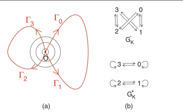
Figure 1. Example7: (a) homoclinic trajectories toO. (b) Corresponding topological Markov graphsG−_KandG+_K.

Theorem 6. There exists1 > 0such that for any0 < < 1 there exists a cross-section N ∈ TR2 _{on the energy level{E =}for whichA}

:= N∩ is a uniformly hyperbolic invariant set with Lyapunov exponents of orderln||−1_{for the Poincar´e mapP. The restriction} ofPtoAis topologically conjugate to the topological Markov chainG+K.

We remark that, by the above two theorems and a result of Fathi [27], the upper

box-counting dimension ofAis at most of order 1/ln||−1.

To illustrate the admissibility condition we give two examples.

Example 7. Suppose the potentialV has a non-degenerate circular local maximum pointOfor

whichV (O)=0 with four homoclinic trajectories toO, as in figure1. Denote the homoclinic

trajectory traversing clockwise to the right ofOby₀, and the one traversing anti-clockwise to

the right ofOby1(namely the time-reverse of0). The other two traversing clockwise and

anti-clockwise to the left ofOare denoted by2and3, respectively. LetK = {0,1,2,3}.

We obtain the indicated graphsG±_K of admissible transitions for energy above or below 0.

Example 8. Suppose the potentialV has three non-degenerate local maximaO0,O1andO2

withV (O0)=V (O1)=0 andV (O2) > 0 as in figure2. LetOmax = {O0, O1}(excluding

O2). SupposeO0 is elliptic andO1is circular. Suppose there is a heteroclinic trajectory0

emanating fromO0toO1and its time-reverse1fromO1toO0. Assume there is a homoclinic

trajectory2 toO1and a ‘bounce’ timessuch that2(s)is not a critical point and that the

trajectory meets perpendicularly the level setV−1(0)at2(s). (It is clear that ¨2(s) = 0,

˙

2(s)=0, and ˙2(t )=0 for−∞< t =s <∞; also d

2

dt2V (2(s)) <0.) SupposeO1has

two other homoclinic trajectories as in figure2,3traversing clockwise and its time-reverse

4. Also assume that O0 has two homoclinic trajectories going out and coming back on

opposite sides of the long axis,5traversing clockwise and its time-reverse6, as in figure2.

LetK= {0,1,2,3,4,5,6}. We obtain the indicated graphsG±_Kof admissible transitions for

energy above or below 0.

To apply our theorems to these sorts of example, we need also to verify non-degeneracy

hypotheses on the homoclinic or heteroclinic trajectories. We will address this in the

3 5

6

1 0

2

4

G+_K

6 1 5 0 2 3 4 G-_K

0 1

5 6

2 3 4

O0

O 2 V (0) -1

O1

Figure 2. Example8: heteroclinic and homoclinic trajectories toO0 andO1 and topological Markov graphsG−_KandG+

K.

(a) (b) (c) (d) (e)

(f ) (g) (h) (i) (j) (k) (l )

Figure 3. Trajectories asymptotic to a local maximum pointO. A circle or ellipse is used to indicate whether the hyperbolic equilibrium(O,0) ∈ T∗R2 _{has equal or distinct eigenvalues} 0< µ1µ2. The long axis of the ellipse is parallel to the projection of the eigen-direction of

µ1to the configuration plane. The circle or ellipse also indicates an equipotential curve of the potentialV.

We have mentioned that the dynamics in the vicinity of the peaks of the potential V

play a crucial role in the bifurcation. LetO∈ Omax. Depending whether the eigenvalues of

(O,0)∈T∗R2_{are equal or not, there are 12 possibilities for how a pair of trajectories meet at}

−3 −2 −1 0 1 2 3

−3

−2

−1 0 1 2 3

x

y

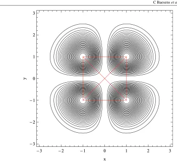
Figure 4.Level sets of the potentialV of form (1) and heteroclinics.

the admissibility condition forE < 0. Possibilities (d), (e) and (k) fulfil the admissibility

condition forE >0. The remaining possibilities (c), (h), (i), (j), and (l) are excluded from

our admissibility condition. Some of them have been addressed by [37].

Now we are in a good position to look again at the results of [6,7]. With the potential

of form (1), the straight lines{(x, y)|x = ±1},{(x, y)|y = ±1}and{(x, y)|y = ±x}are

invariant under the Lagrangian flow (see figure4). Thus, there are 12 heteroclinic trajectories

to the circular maximum points(±1,±1)of the potential (circularity can be proved by direct

calculation of the quadratic part; alternatively the sides of the square form orbits and so the reflection symmetry across the diagonal forces the quadratic part to be circular). We prove in

example17that these heteroclinics are non-degenerate. Hence, by theorem5, we are able to

prove that, whenEdecreases throughEc=e−2, there is an abrupt bifurcation to a subshift

on 4 symbols, say 0, 1, 2 and 3, representing the peaks.

We do not, however, obtain the whole of the subshift that Bleheret alclaim [6], namely that

with forbidden words{00},{11},{22}and{33}, call itBGO. This is because the possibility

(c) (‘90-degree turn’) is not covered by our general approach (it was already perceived as

problematic in [6]). Our subshifthas forbidden words{00},{11},{22},{33},{012},{123},

{230},{301},{032},{321},{210}and{103}. The topological entropy ofBGOis ln 3, while

that of is ln(1 +√2)(this is a relatively simple calculation, based on using symmetry to

reduce the equation for the largest eigenvalue of the adjacency matrix for the graph to that for

a 2×2 matrix). It is conceivable that the subshiftBGOoccurs as soon asE < Ec, because

would be very weakly hyperbolic forE nearEc. Alternatively, it is possible, indeed likely,

that one does not obtain the whole ofBGOstraightaway. Instead, orbits are probably added

gradually toas energy decreases, to make upBGOat some lower energy.

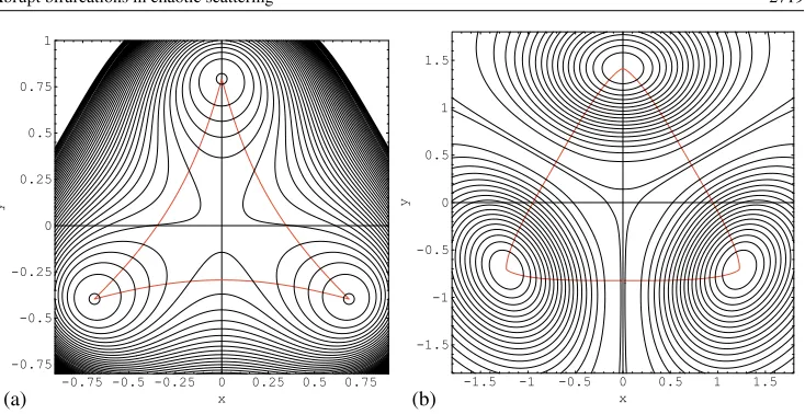
Potential (2) has a maximum point at(0,√2), and numerical computation shows that

the eigenvalues of the Hessian matrix of the potential there are approximately−1.218 02 and

−2.165 36 (indeed, it is diagonal and easy to show thatVxx =Vyy). Hence, the maximum

point is elliptic. Its short axis points towards the centre and numerically there are heteroclinics

coming in along the long axes (look ahead to figure8(b)). This means that we cannot deduce an

abrupt bifurcation when the energy is lowered through the critical valueEc. Instead the most

one can hope for is gradual formation of a full chaotic set as the energy goes sufficiently below

Ecso that the dynamics does not notice that the axes are the wrong way round. We did not prove

that there are heteroclinic connections, but their existence could be proved by minimizing the Jacobi length of absolutely continuous curves connecting the maximum points inside a bounded

region, using compactness and showing the gradient vector∇V points inwards on the boundary.

Furthermore they will come out along the long axes (as in cases (f), (k) in figure3) because

the short axes give only reflection symmetric orbits, which go to infinity. Presumably we could also show that they come in on opposite sides of the maxima as our numerical computation

indicates in figure8(b), but we did not invest time in this. Interestingly, what theorem4would

give in this setting is two periodic orbits for energy slightly aboveEc, rotating in opposite

directions round the triangle formed by the heteroclinic connections.

In examples12and14, to come in section3, we provide two potentials that do exhibit

abrupt bifurcation. For these examples, we rigorously prove the existence and non-degeneracy of heteroclinic trajectories, and the absence of bounded trajectories for energy above the

maximum. Other examples that could be studied using our results are those of [24,25].

3. Non-degeneracy conditions and examples

Define

ME:= {x ∈R2|V (x)E} (i.e. Hill’s region)

and let

J (γ ):= 1

0

2(E−V (γ (s)))|γ (s)˙ |ds (5)

be the Maupertuis functional on the setW1,1of absolutely continuous curves [14]γ : [0,1]→

ME with fixed endsγ (0)andγ (1). The functional is independent of the parametrization of

the curve, and

J (γ )=

γ

∂L

∂v(x, v), v

dt =

p,dγ (6)

withv=γ˙, ifγ is parametrised in such a way that

|γ˙|2

2 +V (γ )=E. (7)

The Maupertuis principle says that ifγ is a trajectory of (3) of energyE, then it is a critical

point ofJ, and conversely, any critical point ofJ becomes a trajectory of energyEafter

reparametrizing as in (7). Alternatively, one could restrict to energyEby considering critical

points ofS = ₀τ(L+E)dt with free duration τ. This has the advantage of allowing a

more general form of LagrangianL. Nevertheless we do not need that generality here and

SupposeOe ∈ Omax. In the phase spaceT∗R2, the hyperbolic equilibrium(Oe,0)has

two-dimensional local stable and unstable manifoldsW_loc± [31]. SinceW_loc± are Lagrangian

manifolds and locally project diffeomorphically to the configuration plane [28], they are defined

byC2_{generating functionsS}±_{on a sufficiently small neighbourhoodU}

eofOe:

W_loc± =(x, p)|p= ∓∇S±(x), x∈Ue .

The functions S± have a non-degenerate minimum at Oe; without loss of generality

S±(Oe)=0.

For anyx ∈Ue, there exists a unique trajectoryω+x : [0,∞)→ Uesuch thatωx+(0)=x

and limt→∞ωx+(t )=Oe. Similarly, there exists a unique trajectoryω−x :(−∞,0]→Uesuch

thatω−_x(0)=xand limt→−∞ω−x(t )=Oe. Then,

S+(x) =

_∞

0

L(ω+_x(t ),ω˙_x+(t ))dt,

S−(x)=

0

−∞L(ω −

x(t ),ω˙−x(t ))dt.

Remark thatS+(x)is equal toS−(x)due to time reversibility of the system.

Forx∈Ue, the Maupertuis actionJof the trajectoryω+x(for energy 0) isS+(x)using (6).

Similarly that ofω_x−isS−(x).

Takeδ >0 small enough so that defining

Ue,δ= {x∈Ue|S±(x) < δ}, (8)

thenS±(x)=δfor allx ∈ ∂Ue,δ. We writeUe =Ue,δ. Its boundary∂UeisC2and for all

x∈∂Ue,ωx±intersect∂Ueorthogonally, by the first variation formula, see [8,12].

Supposeδis sufficiently small andOe0,Oe1 ∈Omax. Let

= (M₀, ∂Ue0, ∂Ue1)

:= { ˜γ : [0,1]→M0| ˜γ (0)∈∂Ue0, γ (˜ 1)∈∂Ue1}

be the space of absolutely continuous curves with endpoints in∂Ue0and∂Ue1.

For any γ˜ ∈ with γ (˜ 0) = y and γ (˜ 1) = x, define a curve γ by adding two

segments ω−_y and ω+

x. (We also need to reparametrize the curve so that γ (0) = Oe0 and

γ (1)=Oe1.) Following [8], for any critical pointγof the functionalJon, the curveγ is a

hetero/homoclinic trajectory providedγis reparametrized as (7). Moreover,J (γ )=J (γ )˜ +2δ.

The condition thatγis non-degenerate can be expressed in the following equivalent ways.

(1) γis a non-degenerate critical point of the Maupertuis functionalJ :→Ron the subset

of curves with the parametrization (7), where

=(M0, Oe0, Oe1)= {γ : [0,1]→M0|γ (0)=Oe0, γ (1)=Oe1}

is the space of absolutely continuous curves with fixed boundary pointsOe0andOe1.

(2) γ is the concatenationω−_{γ (0)˜} · ˜γ ·ω+_{γ (1)˜} andγ˜ is a non-degenerate critical point of the

Maupertuis functionalJ :→Ron the subset of curves with the parametrization (7).

(3) Any point(γ , τ )˜ ∈×R+_{defines a curveu˜: [0, τ]→M}

0byu(t )˜ = ˜γ (t /τ ). Let

G(u, τ )˜ =

τ

0

L(u(t ),˜ u(t ))˙˜ dt

be its action. Thenγis non-degenerate ifγ =ω−_{γ (0)˜} · ˜γ·ω_{γ (1)}+_˜ and(u, τ )˜ is a non-degenerate

C = D

D

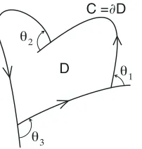
Figure 5. A simple closed curve formed by three pieces of trajectories. The angles turned are measured anti-clockwise, similarly to the external angles of a polygon.

(4) Defineu : R → M0satisfying limt_→−∞u(t ) = Oe0 and limt→∞u(t ) = Oe1 with the

parametrization (7) obtained from a critical pointγ of the Maupertuis functional. Thenγ

is non-degenerate if the unique (up to a scalar multiple) solutionξof the linearized Euler–

Lagrange equation along the hetero/homoclinic trajectoryusatisfying limt→±∞ξ(t )=0

is ˙u.

We will find it convenient to use the following sufficient (but not necessary) condition

for non-degeneracy. Equipped with the Jacobi metric√2(E−V (x))|dx|, geodesics in Hill’s

regionMEare trajectories of the Lagrangian system with potentialV and energyE, and vice

versa. The Jacobi metric is a Riemannian metric which degenerates on the boundary∂ME.

The Gaussian curvatureKE(x)ofxinMEis

KE(x)= − 1 4

ln(E−V (x)) E−V (x)

=1

4

V (x) (E−V (x))2 +

|∇V (x)|2 (E−V (x))3

, (9)

whereis the Laplacian operator, that is,V (x)means the trace of the Hessian ofV. To show

a heteroclinicγ is non-degenerate it suffices that the Gaussian curvature in a neighbourhood

of{γ (t )|0< t <1}be negative.

The following result, which will be useful later for proving absence of bounded trajectories forE > Ecin examples12and14, is a Jacobi metric version of the Gauss–Bonnet formula.

(See figure5.)

Theorem 9 (The Gauss–Bonnet formula). SupposeC is a simple closed piecewise smooth

curve consisting ofmpieces of trajectories (m1). Letθ1,θ2, . . . , θmbe the angle turned at each point where there is a velocity discontinuity. Then

±2 D

KE(x)(E−V (x))dS+ m

i=1

θi = ±2π,

with plus sign ifCis anti-clockwise, or minus sign otherwise, whereDis the region bounded byC.

Proof.The curvatureκ(x)of a trajectory is given by

κ(x)=∇⊥V (x)

|x˙|2

= ∇⊥V (x)

2(E−V (x))

= −1

where∇_⊥V (x)means∇V (x)· ˆnwithnˆthe unit tangent vector perpendicular to ˙x satisfying

ˆ

n×x˙ = |x˙|ˆk(in the usual(ˆi,j ,ˆ k)ˆ -Euclidean coordinates). SupposeC =γ1·γ2· · ·γmis a

product ofmpieces of trajectories, withγ1= {x1(t )|t10t t11},γ2 = {x2(t )|t20tt21},

etc. Then by Green’s theorem the angle turned by these trajectories alongCis±2π−m_i=1θi:

±2π− m

i=1 θi =

t1 1

t0 1

κ(x1)|x˙1|dt+· · ·+ t1

m

t0

m

κ(xm)|x˙m|dt

=

C

κ(x)|dx|

= −1

2

C

∇⊥ln(E−V (x))|dx|

= ∓1

2 D

ln(E−V (x))dS (10)

= ±2 D

KE(x)(E−V (x))dS,

where dSis an element of surface area inD, and (10) takes the minus sign if the trajectory

traversesCanti-clockwise, the plus sign otherwise.

Corollary 10. SupposeKEis non-positive.

(i) Any trajectory of energyEcannot self-intersect.

(ii) Any two distinct trajectories of energyEcan intersect at most once.

Example 11.

(a) For the system of two uncoupled pendula

L((x1, x2), (x˙1,x˙2))=₂1(x˙12+ ˙x22)−(cos 2π x1−1)−(cos 2π x2−1),

(x1, x2)∈R2/Z2,

there are four non-degenerate homoclinic trajectories to(0,0), along the sides of the

unit square in both directions, and a continuum of degenerate homoclinic orbits from one

corner to the diagonally opposite one, see [3,11]. Any pair of non-degenerate homoclinics

joining at(0,0)behave like case (c) or (e) in figure3.

(b) Similarly, all except four homoclinic trajectories to(0,0)for the Lagrangian

L((x1, x2), (x˙1,x˙2))=₂1(x˙12+ ˙x22)+x12−x14+ 2x22−2x24, (x1, x2)∈R2

are degenerate. Any pair of non-degenerate homoclinic orbits joining at the origin behave

like case (h), (i), (k) or (l) in figure3.

Example 12. The Lagrangian system with potential

V (x, y)= −3x2y+y3−(x2+y2)2

(see figure6(a)) has the following properties:

(o) V has three maxima(0,3/4),(−3√3/8,−3/8)and(3√3/8,−3/8), and they are elliptic

with long axes towards the origin.

(i) There exist precisely 6 heteroclinic trajectories between the maxima. They are confined to the equilateral triangle with vertices the three maxima. Their connections behave like

-0.75 -0.5 -0.25 0 0.25 0.5 0.75 1 x

-0.75 -0.5 -0.25 0 0.25 0.5 0.75 1

y

(a) -1 -0.5 0x 0.5 1

-1 -0.5 0 0.5 1

y

(b)

Figure 6. (a) Level sets of the potentialV in example12and heteroclinics forming a cusped triangle. (b) Level sets of the curvatureK27/256with value below 100. Darker shading indicates negative curvature, lighter shading indicates positive curvature, and the level set of zero curvature is the three straight lines through the hilltops plus the origin. Note that for each potential hill top there are two sectors of approach in which the curvature is positive and two in which it is negative.

0

1

2

G

-Figure 7.Markov graphG−for examples12and14.

(ii) All the heteroclinic trajectories are non-degenerate.

(iii) For any energyE, all bounded trajectories are confined to the equilateral triangle.

(iv) ForE > Ec=27/256, there are no bounded trajectories.

(v) ForE =Ec, the only bounded trajectories are the equilibria and heteroclinics between

them.

(vi) There isδ >0 such that for allE∈(Ec−δ, Ec)there is a hyperbolic suspended subshift

corresponding to the Markov graphG−of figure7.

Proof.

(o) To find the maxima is simple calculus. The eigenvalues of the Hessian matrix of the

potential evaluated at the maxima are−27/4 and−9/4, thus the maxima are elliptic.

(i) Minimize the Jacobi length from one maximum to another over the set of absolutely continuous curves contained in the equilateral triangle. The minimum is achieved, by compactness of the set. The result is a geodesic provided it does not include any segment

on the boundary. Suppose there is a segment on the lower boundary {(x, y)| |x| <

which includes the lower boundary. So we can achieve a reduction in the Jacobi length by pushing the curve into the interior of the triangle. Because the eigenvectors of the smaller eigenvalue point to the centre of the triangle, the heteroclinics meet at any of the maximum

points like case (g) in figure3. The heteroclinic orbit from one maximum to another is

unique by the hyperbolicity to be shown in (ii) and the constraint (v) that they must lie in

the triangle. The six heteroclinics found numerically are illustrated in figure6(a) (they

occur in pairs in opposite directions).

(ii) It suffices to show that the Gaussian curvature is negative in the interior of the equilateral

triangle minus the origin (which the heteroclinics do not visit). Direct calculation

shows that

K_27/256(x, y)= −(x

2_+y2₎₍3 8+y)(

3 4 +

√

3x−y)(3₄−√3x−y)

2(₂₅₆27 + 3x2_y−_y3_+(x2_+y2₎2₎3 .

Thus, the zero set of the curvature consists of the three straight lines through the maxima plus the origin, and the curvature is negative inside the triangle, except at the centre. The

curvature has a singularity at the maximum points. See figure6(b).

(iii) We show that for anyE, any trajectory that leaves the equilateral triangle will go to infinity.

For the region{0x−√3y, y−3/8}, a simple calculation shows that

∂V (x, y)

∂y = −3x

2_{+ 3y}2_−4y(x2_+y2₎

−3x2+x2+ 43 8

x2+x 2

3

(with equality only if(x, y)=(3√3/8,−3/8)

=0.

So the force has negative vertical component in the region. When a particle leaves the

triangle from a point on the segment {0 x 3√3/8, y = −3/8}, the vertical

component of its velocity must be non-positive. Hence, the vertical component of the particle’s velocity will always stay negative and bounded away from zero. Therefore, the

particle goes to infinity. (For trajectories that cross the lines{x =0}or{y = −x/√3},

use the symmetry of the system.)

(iv) We have shown thatK27/256(x) <0 whenx is in the interior of the equilateral triangle

minus the origin. It follows thatKE(x) < 0 for allx in the triangle whenE > Ec =

27/256. To see this,K_27/256(x) <0 implies from (9) that(Ec−V )V −|∇V|2 at

x, which implies that(E−V )V <−|∇V|2_{atxfor allE > E}

c(becauseEc> V (x)

soV < 0). Suppose there is a bounded trajectoryγ. It has to lie within the triangle, so must have an accumulation point in phase space (since the part of the energy level that projects to the configuration space in the triangle is compact). The accumulation point

cannot be an equilibrium becauseE > Ec. This implies that there isµ0 andt1 < t2

such that max{|γ (t2)−γ (t1)|,|γ (t˙ 2)−γ (t˙ 1)|}< µ(the velocity atγ (t1)andγ (t2)are

in almost the same direction). Ifµis zero,γ is a periodic trajectory, contradicting (i) of

corollary10. Ifµis not zero, one can takeµsufficiently small so that there is a segment

ν of another trajectory connectingγ (t1)andγ (t2). (This can be done sinceE > Ec.)

The two segments{γ (t )|t1 t t2}andν form a simple closed curve sinceγ cannot

self-intersect (by (i) of corollary10). But, this contradicts (ii) of the corollary. (Remark:

alternatively, one can prove this assertion by proposition13.)

(v) The equilateral triangle can be decomposed into six right triangles of the same area and

In this one, we have

∂2V

∂y∂x(x, y)= −2x(3 + 4y)0,

with the last equality only whenx=0. And

∂V ∂x(x,

−x

√

3)= −2x

2

−√3 +8

3x

0

on the hypotenuse{(x, y)|0 x 3√3/8, √3y = −x}, with the last equality only

whenx =0 orx =3√3/8. This means that in the interior of the right triangle the force

always has negative horizontal component, and implies that a particle in the interior must go to and cross the boundary of the right triangle unless it is asymptotic to the maximum

point(3√3/8,−3/8). If its trajectory is asymptotic to the maximum point, then consider

it in the opposite time direction. If in the opposite time direction it is also asymptotic to a maximum point, it is a heteroclinic. It cannot be a homoclinic because then it would contain a loop, thus it, or another homoclinic by symmetry of the system, must have a

point with zero horizontal velocity. (The case like2in figure2(a) cannot happen here).

Due to the negative horizontal force, the particle cannot go the maximum point. When

the particle crosses the lower boundary{(x, y)|0 x 3√3/8, y = −3/8}, it has to

go to infinity. When it crosses the side{(x, y)|x =0,−3/8y0}or the hypotenuse

to another right triangle, by (ii) of corollary10, it cannot come back to the original right

triangle. Hence, the particle will cross the segment{(x, y)|x = 0,−3/8 y 0}

twice or cross the boundary of the equilateral triangle. The former case contradicts (ii) of

corollary10, while the latter results in an unbounded trajectory.

Part (vi) is a consequence of theorem3.

Proposition 13. ForE > Ec, if there is a bounded trajectoryγ in the configuration space there is one with a self-intersection.

Proof. Let be the phase space orbit corresponding toγ. is bounded so take a limit

pointAofand its orbit. Thenconsists of limit points of, so is bounded. If it has

no self-intersections, take a limit pointB. Denote the projections to configuration space of

all the above by the corresponding lower case letters. The velocity in configuration space

is non-zero atb because E > Ec. Take a local transverse sectionσ throughb. Thenγ

cutsσ repeatedly and these intersections are themselves limit points ofγ. As in the proof of

the Poincar´e-Bendixson theorem, successive intersections of a non-self-intersecting trajectory

withσ are monotonic and thus γ forms a closed curve, which contradicts its having no

self-intersections.

Example 14. The Lagrangian system with potential

V (x, y)= −3x2y+y3−(x2+y2)3

(figure8) has the following properties:

(o) V has three maxima(0,2−1/3_),(−2−4/3√_3,−2−4/3_)and(2−4/3√_3,−2−4/3_{)and they are}

circular.

(i) There exist exactly six heteroclinic trajectories between the maxima and their connections

behave like case (b) in figure3.

(iii) For any energy E, all bounded trajectories are confined to the equilateral triangle with vertices the three maxima.

(iv) ForE > Ec=1/4, there are no bounded trajectories.

(v) ForE=Ec, the only bounded trajectories are the equilibria and the heteroclinics between

them.

(vi) There isδ >0 such that for allE∈(Ec−δ, Ec)there is a hyperbolic suspended subshift

based on the graph of figure7.

Proof.

(o) To find the maxima is simple calculus. The eigenvalues of the Hessian of the potential at

the maximum points are double, equal to−9/21/3_{, thus the peaks are circular.}

(ii) On the energy level{E=1/4}, trajectories of the Lagrangian system are geodesics of the

Jacobi metric√2(E−V (x, y))|d(x, y)|. Letz=x+ iy. Then in the complexz-plane

the metric can be written asρ(z)|dz|with

ρ(z)= |√2z3+ i/√2|.

Note that the metric degenerates only at the hilltopsz1 =2−1/3eiπ/2,z2 =2−1/3ei7π/6and

z3 =2−1/3ei11π/6. Furthermore, the metricρ(z)|dz|corresponds to the Euclidean metric

|dw|in thew-plane where

w(z)=√2z4/4 + iz/√2. (11)

Since all geodesics in thew-plane with the metric|dw|are Euclidean straight lines, all

trajectories for the Lagrangian system are non-degenerate.

(i) Note that heteroclinics correspond to the straight lines joining the three pointsw(z1),

w(z2)andw(z3), thus can be obtained by solving the quartic equation (11) forzand

choosing the right solution. (See figure8(a)). Pointsz1,z2 andz3 are located at the

vertices of an equilateral triangle. The mappingz→whas 2π/3 rotation symmetry, thus

w(z₁),w(z₂)andw(z₃)are also located at the vertices of an equilateral triangle. Taking

Taylor expansion aroundz₁,z₂andz₃, we see that the heteroclinics meet at an angle of

π/6 atz1,z2orz3. (iii) Note that

∂

∂yV (x, y)= −3x

2_{+ 3y}2_−6y(x2_+y2₎2_,

and

− ∂

∂yV (x,−2

−4/3_{)= −3×2}−1/3_(x2_−3×2−8/3₎2_.

The latter is negative except whenxis at a maximum point. The second partial derivative

∂2

∂y2V (x, y)=6y−6(x

2_+y2₎2_−24y2_(x2_+y2₎

is negative wheny is negative. Hence−∂

∂yV (x, y)in the region{(x, y)|y −2− 4/3_}

is negative except at a maximum point. In particular, it is negative in the region

{(x, y)|0x −√3y, y −2−4/3_{}except at a maximum point. The rest of proof is}

similar to that of (iii) of example12.

(iv) It can be verified that the Gaussian curvature K1/4 is everywhere zero except at the

maximum points, where it has a singularity. Thus, from (9),(Ec−V )V = −|∇V|2

everywhere. SinceV < Ecexcept at the maxima, we deduce thatV <0 except at the

critical points ofV (the maxima and the origin), and soKEis everywhere negative when

-0.75 -0.5 -0.25 0 0.25 0.5 0.75 x

-0.75 -0.5 -0.25 0 0.25 0.5 0.75 1

y

(a)

-1.5 -1 -0.5 0 0.5 1 1.5 x

-1.5 -1 -0.5 0 0.5 1 1.5

y

(b)

Figure 8.(a) Level sets of the potentialVin example14and heteroclinics. (b) Level sets of the potential of form (2) and heteroclinics.

(v) All trajectories can be obtained from straight lines in the complexw-plane.

(vi) is a consequence of theorem3.

Remark 15. The logarithm of the absolute value of an analytic function is automatically

harmonic, but it is easily checked explicitly, as follows. Writeρ(z)=ρ(x+ iy)asρ(z,ˆ z)¯ . It

is easy to verify that the Gaussian curvature

K(z)= ˆK(z,z)¯ = −lnρ(z,ˆ z)¯

ˆ

ρ2_(z,z)¯

of any point other thanz1,z2andz3in the complexz-plane with the metricρ(z)|dz|is zero,

since

lnρ(z,ˆ z)¯ =4 ∂ 2

∂z∂z¯lnρ(z,ˆ z)¯

=2 ∂ 2

∂z∂z¯

ln

_√

2z3+√i

2

+ ln

_√

2z¯3−√i

2

=0.

Remark 16. One thing we did not prove in examples12and14is that the set of bounded

orbits forE∈(Ec−δ, Ec)is not more than the constructed subshift. This could probably be

done with a bit more work, see [22].

Example 17. For the Lagrangian system with potential of form (1), there are 12 heteroclinic

trajectories to the four maximum points(±1,±1). They are given by straight lines{(x, y)| −

1x 1, y= ±1},{(x, y)|x = ±1, −1y1}and{(x, y)| −1x = ±y 1}, as

in figure4. All of them are non-degenerate.

Proof. Along the trajectory(x_∗(t ), y_∗(t ))from(−1,1)to(1,1), the orthogonal component of the linearized Euler–Lagrange equation is

d2

dt2(δy)=4x

2

∗ e−(x 2

The coefficient in the right hand side of the equality is positive except whenx_∗passes through

zero. Thus there are no bounded solutions other thanδy=0.

For the trajectory(x_∗(t ), y_∗(t )) from (−1,1) to(1,−1), put u = (x +y)/√2, v =

(x−y)/√2. Then(u_∗(t ), v_∗(t ))is a trajectory from(0,−√2)to(0,√2)in the(u, v)-plane.

The orthogonal component of the linearized Euler–Lagrange equation along(u_∗(t ), v_∗(t ))is

d2

dt2(δv)=u

2

∗

1 + u

2

∗

2

e−u2∗_δv.

The coefficient on the right hand side is positive except whenu_∗ passes through zero. Thus

there are no bounded solutions other than zero. The non-degeneracy of all other heteroclinics

follows from the symmetry of the system.

4. Boundary value problem

This section is devoted to the dynamics of a particle moving in a small neighbourhood of a

non-degenerate local maximumOe∈Omaxof the potentialV. We choose the neighbourhood

to beUe =Ue,δdefined in (8). In this section all results are local, so we omit the subscript

ein the rest of this section. As in [4,9,11,12,32], lemmata18,19,20and proposition21

stated below characterize the main features of the dynamics. For the trajectoriesω_x±(t ), let

z±_x(t )∈W_loc± be the corresponding orbits in the phase space.

Recall that for critical points ofJ(5), parametrized to achieve (7),J has the value

S=

b

a

(L+E)dt,

where [a, b] is the corresponding time-interval.

Proof.From the parametrization (7),√2(E−V )= |γ˙|so

J =

b

a

|γ˙|2dt

=

b

a

1 2|γ˙|

2_−V

+

1 2|γ˙|

2_+V

dt =S.

Lemma 18. There existsT >0large, such that for anyx,y ∈U and anya < b∈ Rwith b−a T, the Lagrangian system (3) has a unique trajectoryq(t ) satisfying q(a) = x, q(b)=y, andq(t )∈Ufora t b. Furthermore,

• ifq is written as a function of(x, y, a, b, t ), then it is aC2function; in fact, it has the phase space representation

(q(t ), p(t ))=z+_x(t−a)+z−_y(t−b)+φ (x, y, a, b, t )eµ1(a−b)_{, (12)}

whereφis a uniformly boundedC2_{function toT}∗_R2∼_=R4_.

• the action

S(x, y, a, b)=

b

a

(L(q(t ),q(t ))˙ +E)dt

isC2_and

S(x, y, a, b)=S+(x)+S−(y)+R(x, y, a, b)eµ1(a−b)_+(b−_a)E,

The representation (12) indicates thatq(t )→ω+

x(t−a)asb→ ∞, thatq(t )→ω−y(t−b)

as a → −∞, and thatq(t ) → O as a → −∞ andb → ∞, all uniformly on compact

time intervals. Since the cotangent planesT_x∗UandT_y∗Uintersect transversally the invariant

manifoldsW_loc± of the hyperbolic equilibrium(O,0), lemma18is a consequence of lemma19

below by puttingYv = Tx∗U andYu = Ty∗U. Lemma19can be derived from Shilnikov’s

lemma [34] or from the strongλ-lemma [19].

Lemma 19. Letgt be the phase flow of the differential equationz˙ =G(z), whereGis aC3 vector field onRn_andg

0 ≡id. Suppose that the origin0is a hyperbolic equilibrium with nonempty local stable and unstable manifoldsW_loc±, and thatµ=min|Re(SpecDG(0))|. Let YuandYvbeC2manifolds intersecting transversallyW_loc− andW_loc+, respectively, at pointszu andzv. Then for sufficiently largeT >0and anya < bwithb−a > T, there exists a unique solutionz(t )=gt(z(a))such that

• z(a)∈Yv,z(b)∈Yu,

• it has the representation

z(t )=gt−a(zv)+gt−b(zu)+ eµ(a−b)φ (a, b, t ), (13)

whereφis a uniformlyC2_{function toR}n_{. If the manifoldsY}

uandYvdepend smoothly on a parameter taking values in a compact manifold, thenφis a uniformly bounded jointC2 function with that parameter.

Proof. The proof follows closely that in [12]. Setz=(u, v)and use coordinatesu∈ W_loc−,

v ∈ W_loc+ in a neighbourhoodN =W_loc− ×W_loc+ of the origin. SupposeYuis the graph of a

function:Yu= {(u, v)|u=f (v)}andgt(Yu)∩Nis given by{(u, v)|u=ft(v)}. Thenzu=

f₀(0)=f (0). The strongλ-lemma [19] says thatftC2 Ceµt,t 0, for some constant

C. An analogous estimatehtC2 Ce−µt also holds forg_t(Y_v)∩N = {(u, v)|v =h_t(u)}

fort 0, withYv = {(u, v)|v =h(u)}andzv =h0(0)=h(0). The boundary conditions

requirez(t ) = gt−a(Yv)∩gt−b(Yu). Thus, any point on the set{z(t )|a t b}satisfies

u = ft₋b(v)andv = ht₋a(u). By the above estimates and the implicit function theorem,

equationv=ht₋a(ft₋b(v))has a unique solutionv(t )=gt₋a(zv)+η(a, b, t )foratb.

The fact that

(0, v(t ))=gt−a(zv)+(0, ht−a(ft−b(v)))−(0, ht−a(0))

=gt−a(zv)++a,b,t(v)

gives+

a,b,tC2 C2eµ(a−b) and+_a,b,t is quadratically small providedht₋a andft₋b are

small:+_a,b,tC2ht−aC2ft−bC2. Hence|η(a, b, t )|C2eµ(a−b). A similar inequality

holds for the derivative ofηina,b,t. The representation (13) is proved for the coordinatev.

The proof is similar for the coordinateu. WhenYuandYvdepend on a parameter, the estimate

above will be uniform in such a parameter.

Let

ζ+(x):= lim t_→∞e

µ1t_ω˙+

x(t ), ζ−(y):=_tlim

→−∞e −µ1t_ω˙−

y(t ).

Lemma 20. The energyh(x, y, a, b)of the trajectoryq(t )is aC2_{function and has the form}

h(x, y, a, b)=eµ1(a−b)_2ζ+_{(x), ζ}−_(y)+h

1(x, y, a, b)

,

Note thatζ+_(x)andζ−_{(y)are tangent vectors atOto the asymptotic trajectoriesω}+ xand

ω−_y, respectively. In other words, write

ζ+(x)= |ζ+(x)|ξ+(x), ζ−(y)= |ζ−(y)|ξ−(y),

then

ξ+(x):= lim t→∞

˙

ω+ x(t )

|ω˙+ x(t )|

, and ξ−(y):= lim

t→−∞ ˙

ω−_y(t )

|ω˙−y(t )| .

For equal eigenvaluesµ1(O)=µ2(O), the scalar productξ+(x), ξ−(y)may take any value

in [−1,1] for a pairxandy ∈U. Whenµ1(O)=µ2(O), letWloc++⊂Wloc+ andWloc−−⊂Wloc−

be one-dimensional local strong stable and unstable manifolds of the hyperbolic equilibrium

(O,0)∈T∗R2, namely the invariant manifolds tangent to the eigenvectors with eigenvalues

±µ2 (the strong directions). The manifolds Wloc±± divideWloc± into connected components:

W_loc+ \W_loc++=W_loc,R+ ∪W_loc,L+ ,W_loc− \W_loc−− =W_loc,R− ∪W_loc,L− . The projectionsπ(W±±)to

configuration space are identical and divide the neighbourhoodUinto connected components

U\π(W_loc±±)=UR∪UL.

Whenµ₁ =µ₂, we haveξ+_{(x), ξ}−_{(y) ∈ {0,±1}. More precisely,}

ξ+(x), ξ−(y) =

−1 if(x, y)∈(UR×UR)∪(UL×UL) +1 if(x, y)∈(UR×UL)∪(UL×UR).

Proof of lemma20.Since we are concerned with the dynamics only in a neighbourhoodUof

O, we may shift and rotate coordinates if necessary so that the origin is located atOand in the

new coordinates (we still usex =(x1, x2)∈R2and conjugate momentump=(p1, p2)∈R2)

the Hessian matrix ofV atOis diagonal and the Hamiltonian takes the form

H (x, p)=1₂|p|2−1₂ν1x12−12ν2x 2

2+O3(x), (14)

where−ν1,−ν2are the eigenvalues of the Hessian matrix ofV atO. Ifν1 =ν2the result was

proved in [9]. Ifν1 =ν2, the eigenvalues of the Hamiltonian dynamics are±µ1,±µ2with

µ1=√ν1,µ2=√ν2. There exists a symplectic transformationT :(x, p)→(u, v)given by

(x1, x2) =T1−1(u, v)

=

u1−µ1v1

√

2ν1

,u2√−µ2v2

2ν2

+O2(u, v),

(p₁, p₂)=T₂−1(u, v)

=

u1+µ1v1

√

2 ,

u2+µ2v2

√

2

+O₂(u, v),

such thatW_loc+ = {u=0},W_loc− = {v=0}, and the Hamiltonian takes the form

H (u, v)=µ1u1v1(1 +O(u, v))+µ2u2v2(1 +O(u, v)). (15)

Ifµ1 < µ2, then the coordinates can be chosen in such a way thatWloc++ = {u=0, v1 =0}

andW_loc−−= {u1=0, v=0}. Hamilton’s equations onWloc− have the form

˙

u1=µ1u1+O2(u), u˙2=µ2u2+O2(u), (16)

where the right hand side of both equations is of class C3. By aC2 change of variables

η = f₋(u) = (f1−(u), f2−(u)), they can be transformed to linear equations ˙η1 = µ1η1, ˙

η2=µ2η2unlessµ2=2µ1[35].

Hence ifµ₂=2µ₁the phase flow onW_loc− takes the form

gt(u,0)=

f₋−1(eµ1t_f

1−(u),eµ2tf2−(u)),0

= eµ1t_((f