Towards automatic model comparison : an adaptive sequential Monte Carlo approach

warwick.ac.uk/lib-publications

Original citation:

Zhou, Yan (Researcher in statistics), Johansen, Adam M. and Aston, John A. D.. (2015)

Towards automatic model comparison : an adaptive sequential Monte Carlo approach.

Journal of Computational and Graphical Statistics, 25 (3). pp. 701-726.

Permanent WRAP URL:

http://wrap.warwick.ac.uk/74069

Copyright and reuse:

The Warwick Research Archive Portal (WRAP) makes this work of researchers of the

University of Warwick available open access under the following conditions.

This article is made available under the Creative Commons Attribution 4.0 International

license (CC BY 4.0) and may be reused according to the conditions of the license. For more

details see:

http://creativecommons.org/licenses/by/4.0/

A note on versions:

The version presented in WRAP is the published version, or, version of record, and may be

cited as it appears here.

Toward Automatic Model Comparison: An

Adaptive Sequential Monte Carlo Approach

Yan Z

, Adam M. J

, and John A.D. A

Model comparison for the purposes of selection, averaging, and validation is a problem found throughout statistics. Within the Bayesian paradigm, these problems all require the calculation of the posterior probabilities of models within a particular class. Substantial progress has been made in recent years, but difficulties remain in the implementation of existing schemes. This article presents adaptive sequential Monte Carlo (SMC) sampling strategies to characterize the posterior distribution of a collection of models, as well as the parameters of those models. Both a simple product estimator and a combination of SMC and a path sampling estimator are considered and existing theoretical results are extended to include the path sampling variant. A novel approach to the automatic specification of distributions within SMC algorithms is presented and shown to outperform the state of the art in this area. The performance of the proposed strategies is demonstrated via an extensive empirical study. Comparisons with state-of-the-art algorithms show that the proposed algorithms are always competitive, and often substantially superior to alternative techniques, at equal computational cost and considerably less application-specific implementation effort. Supplementary materials for this article are available online.

Key Words: Adaptive Monte Carlo algorithms; Bayesian model comparison;

Normal-izing constants; Path sampling; Thermodynamic integration.

1. INTRODUCTION

Model comparison lies at the core of Bayesian decision theory (Robert2007) and has attracted considerable attention in recent decades. Most approaches to the calculation of the required posterior model probabilities depend upon asymptotic arguments, the post-processing of outputs from Markov chain Monte Carlo (MCMC) algorithms operating on the space of a single model or using specially designed MCMC techniques that provide direct estimates of these quantities (e.g., reversible jump MCMC, RJMCMC; Green1995). Within-model simulations are simpler, but generalizations of the harmonic mean estimator

Yan Zhou, Department of Statistics and Applied Probability, National University of Singapore, Singapore (E-mail:[email protected]). Adam M. Johansen, Department of Statistics, University of Warwick, Coventry CV4 7AL, UK (E-mail:[email protected]). John A.D. Aston, Statistical Laboratory, Department of Pure Mathematics and Mathematical Statistics, University of Cambridge, Cambridge CB3 0WB, UK (E-mail:

[email protected]).

©2016 Yan Zhou, Adam M. Johansen, and John A.D. Aston. Published with license by Taylor & Francis. This is an Open Access article distributed under the terms of the Creative Commons Attribution License (http://crea tivecommons.org/licenses/by/4.0/), which permits unrestricted use, distribution, and reproduction in any medium, provided the original work is properly cited.

Journal of Computational and Graphical Statistics, Volume 25, Number 3, Pages 701–726 DOI:10.1080/10618600.2015.1060885

(Gelfand and Dey 1994) that are widely used in this setting require careful design to ensure finite variances and convergence assessment can be difficult. Simulations on the whole model space are often difficult to implement efficiently even though they can be conceptually appealing.

More robust and efficient Monte Carlo algorithms have been established in recent years. Many of them are population based, dealing with a collection of samples at each iteration, including sequential importance sampling and resampling (annealed importance sampling AIS, Neal2001; sequential Monte Carlo SMC, Del Moral, Doucet, and Jasra2006b) and population MCMC (PMCMC; Liang and Wong2001; Jasra, Stephens, and Holmes2007a). However, most studies have focused on their abilities to explore high-dimensional and multimodal spaces. The application of these algorithms to Bayesian model comparison is less well studied. Here, we motivate and present approaches based around the SMC family of algorithms, and demonstrate their effectiveness empirically.

SMC methods are a class of sampling algorithms, which combine importance sampling and resampling. They have been primarily used as “particle filters” to solve optimal filtering problems; see, for example, Capp´e, Godsill, and Moulines (2007) and Doucet and Johansen (2011) for recent reviews. They are used here in a different manner, which were proposed by Del Moral, Doucet, and Jasra (2006b) and developed by Del Moral, Doucet, and Jasra

(2006a) and Peters (2005). This framework employs a sequence of artificial distributions

on spaces of increasing dimensions, which admit the distributions of interest as marginals. Although it is well known that SMC is well suited to the computation of normalizing constants and that it is possible to develop relatively automatic SMC algorithms by em-ploying a variety of “adaptive” strategies, their use for Bayesian model comparison has not yet received a great deal of attention. We highlight three strategies for computing posterior model probabilities using SMC, focusing on strategies that require minimal tuning and can be readily implemented requiring only the availability oflocally mixingMCMC proposals. These methods admit natural and scalable parallelization and we demonstrate the potential of these algorithms with real implementations suitable for use on consumer-grade parallel computing hardware including GPUs, reinforcing the message of Lee et al. (2010). We also present a new approach to adaptation and guidelines on the near-automatic implementation of the proposed algorithms. These techniques are applicable to SMC algorithms in much greater generality. The proposed approach is compared with state-of-the-art alternatives in extensive simulation studies that demonstrate its performance and robustness.

The next section provides a brief survey of Bayesian model comparison literature. Sec-tion3presents three algorithms for performing model comparison using SMC techniques and Section 4 provides several illustrative applications, together with comparisons with other techniques. The article concludes with some discussion.

2. BACKGROUND

feasible to exhaustively summarize this literature here. We describe the major contributions to the area and recent developments of particular relevance.

2.1 ANALYTICMETHODS ANDMCMC

The Bayesian information criterion (BIC), developed by Schwarz (1978), is based upon a large sample approximation of the Bayes factor. An asymptotic argument concerning Bayes factors under appropriate regularity conditions justifies the choice of the model with the smallest value of BIC. Although appealing in its simplicity, justification requires the availability of a large number of observations.

The Bayesian approach to model comparison is, of course, to consider the posterior probabilities of the possible models (Bernardo and Smith1994, chap. 6).

Given a denumerable collection of models{Mk}k_∈K, with modelMkhaving parameter

space k, Bayesian inference proceeds from a prior distribution over the collection of

models,π(Mk), a prior distribution for the parameters of each model,π(θk|Mk) and the

(model-specific) likelihoodp(y|θk, Mk) to the model posterior:

π(Mk|y)=

p(y|Mk)π(Mk)

p(y) , (2.1)

wherep(y|Mk)=

θkp(y|θk, Mk)π(θk|Mk)dθkis termed theevidencefor modelMkand the normalizing constantp(y)=_k∈Kp(y|Mk)π(Mk) can be easily calculated if|K|is

finite and the evidence for each model is available. The case where|K| is countable is discussed later. We first review some techniques for evidence calculation.

Several techniques have been proposed to approximate the evidence for a model using simulation techniques, which approximate the posterior distribution of that model, including the harmonic mean estimator of Newton and Raftery (1994), Raftery et al. (2006), and generalizations thereof (Gelfand and Dey1994). These pseudo-harmonic mean methods use the insight that for any densityg, such thatg(·)p(·|y, Mk), the following identity

holds,

g(θk)

p(y, θk|Mk)

π(θk|y, Mk)dθk=

g(θk)

p(y, θk|Mk)

p(y, θk|Mk)

p(y|Mk)

dθk=

1

p(y|Mk)

(2.2) and by approximating the leftmost integral one can obtain an estimate of the evidence. Unfortunately, considerable care is required in the implementation of such schemes to control the variance of the resulting estimator—see Neal (1994).

In the particular case of the Gibbs sampler, Chib (1995) provided an alternative approach based on the identity,

p(y|Mk)=

p(y|θk, Mk)π(θk|Mk)

π(θk|y, Mk)

, (2.3)

which holds for any value of θk. An estimator of the marginal likelihood can be

ob-tained by replacingθk with a particular value, say θkI, which is usually chosen from the

high probability region of the posterior distribution and approximating the denominator

π(θI

k|y, Mk) using the output from a Gibbs sampler. Though this method does not suffer

sampler mixes adequately. This approach was generalized to other Metropolis–Hastings algorithms, by Chib and Jeliazkov (2001), who required only that the proposal distributions be known.

The RJMCMC strategy first proposed by Green (1995) is undoubtedly the most widespread approach that targets the joint posterior distribution over model and param-eters. RJMCMC adapts the Metropolis–Hastings algorithm to construct a Markov chain on an extended state-space, which admits the posterior distribution over both model and parameters as its invariant distribution. The design of efficient between-model moves is often difficult, and the mixing of these moves largely determines the performance of the algorithm. For example, in multimodal models, where RJMCMC has attracted substantial attention, information available in the posterior distribution of a model of any given dimen-sion does not characterize modes that exist only in models of higher dimendimen-sion, and thus successful moves between those models become unlikely and difficult to construct (Jasra, Stephens, and Holmes2007b). In addition, RJMCMC will not characterize models of low posterior probability well, as those models will be visited by the chain only rarely. In some cases, it will be difficult to determine whether the low acceptance rates of between-model moves result from actual characteristics of the posterior or from a poorly adapted proposal kernel.

A post-processing approach to improve the computation of normalizing constants from RJMCMC output using a bridge-sampling approach was advocated by Bartolucci, Scaccia, and Mira (2006). Sophisticated variants of these algorithms, such as those developed in Peters, Hayes, and Hossack (2010), have also been considered but depend upon essentially the same construction and ultimately require adequate mixing of the underlying Markov process.

Carlin and Chib (1995) presented an alternative method for simulating the model prob-ability directly through a Gibbs sampler on the space {Mk}k_∈K×

k∈Kk. The joint

parameter is thus (M, θ) whereθ is the vector (θk)k∈K and conditional on modelMk the

data y only depend on a subset, θk, of the parameters. To form the Gibbs sampler, a

so-called pseudopriorπ(θk|M=Mk) in addition to the usual priorπ(θk|Mk) is selected,

such that given the model indicatorM, the parameters associated with different models are conditionally mutually independent. In this way, a Gibbs sampler can be constructed pro-vided that all the full conditional distributionsπ(θk|y, θk=k, M) andπ(M=Mk|y, θ) for

k∈Kare available. The performance of this sampler, which was generalized by Godsill (2001), is very sensitive to the selected pseudopriors and sampling from the full conditional distribution must be feasible.

The methods reviewed above either demand substantial knowledge of the target distri-butions or require substantial tuning.

2.2 RECENTDEVELOPMENTS ONPOPULATION-BASEDMETHODS

We consider two broad groups of population-based Monte Carlo methods. One family, including SMC, is based on sequential importance sampling and resampling. Another approach is population MCMC (PMCMC; Geyer1991; Marinari and Parisi1992; Liang and Wong 2001) also known as parallel tempering. PMCMC operates by constructing a sequence of distributions {πt}Tt₌0 withπ0 corresponding to the target distribution and

easy to sample. A population of samples is maintained, with theith element of the population being approximately distributed according toπi; the algorithm proceeds by simulating an

ensemble of parallel MCMC chains each targeting one of these distributions. The chains interact with one another via exchange moves, in which the state of two adjacent chains is swapped, and this mechanism allows for information to be propagated between the chains and hopefully for the fast mixing ofπT to be partially transferred to the chain associated

withπ0. The resulting samples target the product

T

t₌0πt, which admitsπ0as a marginal.

There is substantial interest in the use of population-based methods to explore high-dimensional and multimodal parameter spaces, which challenge conventional MCMC algorithms. Jasra, Stephens, and Holmes (2007a) compared the performance of the two approaches in this context. There is also increasing interest in using these methods for Bayesian model comparison. In principle, PMCMC output can be post-processed in the same way as conventional MCMC to obtain estimates of evidence for each model. However, this approach inherits many of the disadvantages of the basic estimators. Jasra, Stephens, and Holmes (2007b) combined PMCMC with RJMCMC and thus provided a direct es-timate of the posterior model probability. Another approach is to use the outputs from all the chains to approximate the path sampling estimator (Gelman and Meng1998), see Calderhead and Girolami (2009). However, the mixing speed of PMCMC is sensitive to the number and placement of the distributions{πt}T_t=0(see Atchad´e, Roberts, and Rosenthal

(2010) for the optimal placement of distributions in terms of a particular mixing criterion for a restricted class of models). As seen in Calderhead and Girolami (2009), the placement of distributions can be critical—see Section4.

The use of AIS for computing normalizing constants directly and via path sampling dates back at least to Neal (2001); see Vyshemirsky and Girolami (2008) for a recent example of its use in the computation of model evidences. It has often been suggested that more general SMC strategies provide no advantage over AIS when the normalizing constant is the object of inference. Later we will demonstrate that this is not generally true, adding improved robustness of normalizing constant estimates to the advantages afforded by resampling within SMC. This is consistent with theoretical results (Schweizer

2012) obtained in a slightly different context, which show that resampling can qualitatively improve the theoretical behavior of the estimator when the initial and final distributions differ substantially. More details on the use of SMC and path sampling for Bayesian model selection are provided in the next section. The use of PMCMC coupled with path sampling was discussed in Vyshemirsky and Girolami (2008).

Jasra et al. (2008) developed a method using a system of interacting SMC samplers for transdimensional simulation. The targeting distributionπand its spaceSare the same as in RJMCMC. As usual in SMC, a sequence of distributions{πt}Tt₌0with increasing dimensions

are constructed such thatπTadmitsπas a marginal. The algorithm starts with a set of SMC

samplers with equal number of particles; each of them targetsπi,t(x)∝πt(x)I(x ∈Si) up

to a predefined time indextI_{, such that{S}

i}is a partition ofS. At timetI particles from

combined SMC and MCMC via the mechanism of particle MCMC (Andrieu, Doucet, and Holenstein2010) using an SMC algorithm as an RJMCMC proposal. This strategy is likely to lead to better mixing than conventional RJMCMC algorithm but comes at considerable computational cost.

A proof-of-concept study in which several SMC approaches to the problem were outlined was provided by Zhou, Johansen, and Aston (2012) and these approaches are developed below. These strategies based around various combinations of path sampling (Gelman and Meng1998) and SMC (as used by Johansen, Del Moral, and Doucet (2006) in a rare events context and by Rousset and Stoltz (2006) in the context of the estimation of free energy differences) or the unbiased estimation of the normalizing constant via standard SMC techniques (Del Moral1996; Del Moral, Doucet, and Jasra2006b).

A strategy for SMC-based variable selection was developed by Sch¨afer and Chopin (2013); however, this approach depends upon the precise structure of this particular problem and does not involve the explicit computation of normalizing constants.

2.3 CHALLENGES FORMODELCOMPARISONTECHNIQUES

There are a number of desirable features in algorithms that seek to address any model comparison problem and that these desiderata can find themselves in competition with one another. One always requires accurate evaluation of Bayes factors or model proportions and to obtain these one requires estimates of either normalizing constants or posterior model probabilities with small error making the efficiency of any Monte Carlo algorithm employed in their estimation critical. If one is interested in characterizing behavior conditional upon a given model or even calculating posterior-predictive quantities, it is likely to be necessary to explore the full parameter space of each model; this can be difficult if one employs between-model strategies that spend little time in models of low probability. In many settings, end-users seek to interpret the findings of model selection experiments and in such cases, accurate characterization of all models including those of relatively small probability may be important.

3. METHODOLOGY

SMC samplers provide, iteratively, collections of weighted samples from a sequence of distributions{πt}Tt=0over essentially any random variables on some measurable spaces

(Et,Et), by constructing a sequence of auxiliary distributions{πt}Tt=0on spaces of increasing

dimensions,

πt(x0:t)=πt(xt) t−1

s₌0

Ls(xs+1, xs), (3.1)

where the sequence of Markov kernels {Ls}ts−=10, termed backward kernels, is formally

arbitrary but critically influences the estimator variance. See Del Moral, Doucet, and Jasra

(2006b) for further details and guidance on the selection of these kernels.

Standard sequential importance resampling algorithms can then be applied to the se-quence of synthetic distributions,{πt}Tt₌0. At timet=n−1, assume that a set of weighted

particles{W_n(i₋)₁, X(_0:i)_n−1}N

of each particle is extended with a Markov kernel say,Kn(xn−1, xn) yielding the set of

particles{X_0:(i)_n}N_i=1and importance sampling is then applied. The weights are update by a factorwn, termed theincremental weights, calculated as

wn(xn−1, xn)=

πn(xn)Ln−1(xn, xn−1)

πn₋1(xn₋1)Kn(xn₋1, xn)

. (3.2)

Ifπnis only known up to a normalizing constant, sayπn(xn)=γn(xn)/Zn, then we can use

theunnormalizedincremental weights

wn(xn₋1, xn)=

γn(xn)Ln−1(xn, xn−1)

γn−1(xn−1)Kn(xn−1, xn)

(3.3)

for importance sampling. Further, with the previouslynormalizedweights{W_n(i₋)₁}N i=1, we

can estimate the ratio of normalizing constantZn/Zn₋1by

Zn

Zn−1

=

N

i=1

W_n(i₋)₁wn(Xn(i₋)1:n), (3.4)

and

Zn

Z1

=

n

p₌2

Zp

Zp−1

=

n

p₌2

N

i₌1

W_p(i₋)₁wp(X( i)

p−1:p) (3.5)

provides an unbiased (Del Moral2004, Proposition 7.4.1) estimate of Zn/Z1. See Del

Moral, Doucet, and Jasra (2006b) for details on calculating the incremental weights in general; in practice, whenKnisπn-invariant,πnπn₋1, andLn₋1is the associated

time-reversal kernel, the unnormalized incremental weight function becomes

wn(xn−1, xn)=

γn(xn−1)

γn−1(xn−1)

. (3.6)

This will be the situation throughout the remainder of this article.

3.1 SEQUENTIALMONTECARLO FORMODELCOMPARISON

The problem of interest is characterizing the posterior distribution over {Mk}k∈K, a

set of possible models, with model Mk having parameter vector θk∈k, which must

also usually be inferred. Given prior distributionsπ(Mk) and π(θk|Mk) and likelihood

p(y|θk, Mk), we seek the posterior distributions π(Mk|y)∝p(y|Mk). There are three

fundamentally different approaches to the computations:

1. Calculate posterior model probabilities directly.

2. Calculate the evidence,p(y|Mk), of each model.

3. Calculate pairwise evidence ratios.

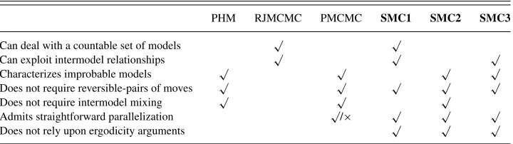
Table 1. Strengths of algorithms for model choice. PMCMC admits a degree of parallelization, but is not a natural candidate for implementation on massively parallel architectures

PHM RJMCMC PMCMC SMC1 SMC2 SMC3

Can deal with a countable set of models √ √

Can exploit intermodel relationships √ √ √

Characterizes improbable models √ √ √ √

Does not require reversible-pairs of moves √ √ √ √ √ Does not require intermodel mixing √ √ √

Admits straightforward parallelization √/× √ √ √ Does not rely upon ergodicity arguments √ √ √

3.1.1 SMC1: An All-in-One Approach. One could consider obtaining samples from the same distribution employed in the RJMCMC approach to model comparison, namely:

π(1)(Mk, θk)∝π(Mk)π(θk|Mk)p(y|θk, Mk), (3.7)

which is defined on the disjoint union spacek_∈K({Mk} ×k).

One obvious SMC approach is to define a sequence of distributions{π_t(1)}T

t=0 such that

π₀(1)is easy to sample from,π_T(1)=π(1)_{and the intermediate distributions move smoothly}

between them. In the remainder of this section, we use the notation (Mt, θt) to denote a

random sample on the spacek∈K({Mk} ×k) at timet. One simple approach is the use

of an annealing scheme such that

πt(1)(Mt, θt)∝π(Mt)π(θt|Mt)p(y|θt, Mt)α(t/T), (3.8)

for some monotonically increasing α: [0,1]→[0,1] such thatα(0)=0 and α(1)=1. Other approaches are possible and might prove more efficient for some problems (such as the “data tempering” approach that Chopin (2002) proposed for parameter estimation—a strategy that would lend itself naturally to “online” estimation of evidence, but that would preclude the use of the path sampling estimator), but this strategy provides a convenient generic approach. These choices lead to Algorithm 1.

This approach might outperform RJMCMC when it is difficult to design fast-mixing Markov kernels. Such an SMC strategy can outperform MCMC at a given computational cost—see, for example, Fan, Leslie, and Wand (2008), Johansen, Doucet, and Davy (2008), and Fearnhead and Taylor (2010). Such transdimensional SMC has been proposed in several contexts (Peters2005) and an extension proposed and analyzed by Jasra et al. (2008).

Algorithm 1SMC1 : An All-in-One Approach to Model Comparison.

Initialization:Sett←0.

SampleX(₀i)=(M₀(i), θ₀(i))∼νfor some proposal distributionν(usually the joint prior). WeightW0(i)∝w0(X

(i) 0 )=π(M

(i) 0 )π(θ

(i) 0 |M

(i) 0 )/ν(M

(i) 0 , θ

(i) 0 ).

Apply resampling if necessary (e.g., if ESS (Kong et al. 1994) less than some threshold).

Iteration:Sett←t+1.

WeightWt(i)∝W

(i)

t−1p(y|θ (i)

t−1, M (i)

t−1)α(t /T)−α([t−1]/T).

Apply resampling if necessary. SampleX(ti)∼Kt(·|X

(i)

t−1), aπ (1)

t -invariant kernel.

We include this approach for completeness and study it empirically later. Like other transdimensional methods, this approach depends upon collection of models being specified in advance. If new models are considered, then the entire simulation must be redone. The more direct approaches described in the following sections lead more naturally to easy-to-implement strategies with good performance.

3.1.2 SMC2: A Direct-Evidence-Calculation Approach. An alternative approach would be to estimate explicitly the evidence associated with each model. We propose to do this by sampling from a sequence of distributions for each model: starting from the parameter prior and sweeping through a sequence of distributions to the posterior.

Numerous strategies are possible to construct such a sequence of distributions, but one option is to use for each modelMk,k∈K, the sequence{πt(2,k)}

Tk

t₌0, defined by

πt(2,k)(θt)∝π(θt|Mk)p(y|θt, Mk)αk(t/Tk), (3.9)

where the number of distributionTk, and the annealing schedule,αk: [0,1]→[0,1] may

be different for each model. This leads to Algorithm 2.

The estimator of the posterior model probabilities depends upon the approach taken to estimate the normalizing constant. Direct estimation of the evidence can be performed using the output of this SMC algorithm and the standard estimator (Del Moral, Doucet, and Jasra2006b, eq. (14)), termed SMC2-DS below:

1

N

N

i=1

π(θ₀(k,i)|Mk)

ν(θ₀(k,i)) ×

T

t=2

N

i=1

W_t(₋k,i₁)p(y|θ_t(₋k,i₁)Mk)αk(t/Tk)−αk([t−1]/Tk), (3.10)

where W_t(₋k,i₁) is the importance weight of sample i, θ_t(₋k,i₁), after any resampling step of iterationt−1 for model Mk. This formula can be simplified by replacing W(

k,i)

t−1 with

1/N when resampling is conducted at every iteration (and it is unbiased); otherwise a mathematically simpler representation less naturally suited to computational use is provided by Del Moral, Doucet, and Jasra (2006b, eq. (15)). An alternative approach to computing the evidence is also worthy of consideration. As has been suggested, and shown empirically to perform well previously (see, e.g., Johansen, Del Moral, and Doucet2006), it is possible to use all of the samples from every generation of an SMC sampler to approximate the path sampling estimator. Section3.2provides details.

The posterior distribution of the parameters conditional upon a particular model can also be approximated using

π_T(2,k)

k (dθ)=

N

i=1

W_T(k,i)

k δθ_Tk(k,i)(dθ).

each model is dealt with in isolation. While this may not be desirable in every situation, there are circumstances in which efficient moves between models are almost impossible to devise.

This approach also has some disadvantages. In particular, it is necessary to run a separate simulation for each model—rendering it impossible to deal with countable collections of models (although this is not such a substantial problem in many interesting cases). The ease of implementation may often offset this limitation.

Algorithm 2SMC2 : A Direct-Evidence-Calculation Approach.

For each modelk∈Kexecute the following algorithm.

Initialization:Sett←0.

Sampleθ₀(k,i)∼νkfor some proposal distributionνk(usually the parameter prior). WeightW0(k,i)∝w0(θ

(k,i) 0 )=π(θ

(k,i)

0 |Mk)/νk(θ (k,i) 0 ).

Apply resampling if necessary.

Iteration:Sett←t+1.

WeightWt(k,i)∝W

(k,i)

t−1p(y|θ (k,i)

t−1, Mk)

α(t /Tk)−α([t−1]/Tk)_.

Apply resampling if necessary. Sampleθt(k,i)∼Kt(·|θt(−k,i1)), aπ

(k,2)

t -invariant kernel.

RepeattheIterationstepuntilt=Tk.

3.1.3 SMC3: A Relative-Evidence-Calculation Approach. A final approach can be thought of assequential model comparison. Rather than estimating the evidence associated with any particular model, we could estimate pairwise evidence ratios directly. The SMC sampler starts with an initial distribution being the posterior of one model (an initial sample could be obtained using a secondary SMC algorithm or other sampler) and moves toward the posterior of another related model. Then the sampler can continue toward another related model and so forth.

Given a finite collection of models{Mk},k∈K, suppose the models are ordered in a

sensible way (e.g.,Mk−1is nested withinMkorθkis of higher dimension thanθk−1). For

each k∈K, we consider a sequence of distributions {πt(3,k)} Tk

t₌0, such thatπ (3,k)

0 (M, θ)=

π(θ|y, Mk)I{Mk}(M) andπ

(3,k)

Tk (M, θ)=π(θ|y, Mk+1)I{Mk+1}(M)=π (3,k₊1)

0 (M, θ). When

it is possible to construct an SMC sampler that iterates over this sequence of distributions, the estimate of the ratio of normalizing constants is the Bayes factor estimate of model

Mk+1in favor of modelMk.

This approach is conceptually appealing, but requires the construction of a smooth path between the posterior distributions of interest. The geometric annealing strategy that has been advocated as a good generic strategy in the previous sections is only appropriate when the support of successive distributions is nonincreasing. This is unlikely to be the case in interesting model comparison problems.

In this article, we consider a sequence of distributions on the disjoint union{Mk, k} ∪

{Mk+1, k+1},with the sequence of distributions{π(3

,k)

t }

Tk

t=0defined as the full posterior,

πt(3,k)(Mt, θt)∝πt(Mt)π(θt|Mt)p(y|θt, Mt), (3.11)

whereMt ∈ {Mk, Mk+1}and the “prior” over models at timet,πt(Mk+1) :=α(t /Tk), for

efficient exploration of the whole model space, only moves between two models are required and the sequence of distributions employed helps to ensure exploration of both model spaces. Algorithm 3 uses this particular sequence of distribution but other sequence of distributions between models could be employed.

An advantage of this approach is that it provides direct estimates of the Bayes factor, which is of interest for model comparison purpose while not requiring exploration of as complicated a space as that employed within RJMCMC or SMC1. The estimation of normalizing constant in SMC3 follows in exactly the same manner as in the SMC2 case. In SMC3, the same estimator provides a direct estimate of the Bayes factor.

Algorithm 3SMC3: A Relative-Evidence-Calculation Approach to Model Comparison.

Initialization:Setk←1.

Use Algorithm2to obtain weighted samples forπ_T(3,1)

1 , the parameter posterior for modelM1

Relative Evidence Calculation

Setk←k+1,t←0.

Denote current weighted samples as{W0(k,i), X (k,i)

0 }Ni=1, whereX (k,i)

0 =(M

(k,i)

0 , θ

(k,i)

0 )

Apply resampling if necessary.

Iteration:Sett←t+1.

WeightWt(k,i)∝W

(k,i)

t−1πt(M

(k,i)

t−1)/πt−1(M (k,i)

t−1).

Apply resampling if necessary. Sample (Mt(k,i), θ

(ki)

t )∼Kt(·|M

(k,i)

t−1θ (k,i)

t−1), aπ (3,k)

t -invariant kernel.

Repeat theIterationstep up tot=Tk.

RepeattheRelative Evidence Calculationstepuntil sequentially all relative evidences are

calcu-lated.

3.2 PATHSAMPLING VIASMC2/SMC3

A Monte Carlo approximation of thepath samplingidentity (Gelman and Meng1998) (also known as thermodynamic integration or Ogata’s method) also provides an estimate of the normalizing constant. The use of AIS for the same purpose (Neal2001) is common in some settings; as will be demonstrated below the incorporation of some other elements of the more general SMC algorithm family can improve performance at negligible cost. Given a parameterαthat defines a family of distributions,{pα=qα/Zα}α_∈[0,1]that move

smoothly fromp₀=q₀/Z₀top₁=q₁/Z₁asαincreases from zero to one. The logarithm of the ratio of their normalizing constants satisfies a simple integral relationship under mild regularity conditions: log Z1 Z₀ = 1 0 Eα

dlogqα(·)

dα

dα, (3.12)

where Eα denotes expectation under pα; see Gelman and Meng (1998). Note that the

sequence of distributions in the SMC2 and SMC3 algorithms above, can both be interpreted as belonging to such a family of distributions, with αt =α(t /Tk), where the mapping

α: [0,1]→[0,1] is again monotonic withα(0)=0 andα(1)=1.

estimator, and this integral can then be approximated via numerical integration. Whenever the sequence of distributions employed by SMC3 has appropriate differentiability, it is also possible to employ path sampling to estimate, directly, the evidence ratio via this approach applied to the samples generated by that algorithm. In general, given an increasing sequence {αt}Tt=0 whereα0 =0 andαT =1, a family of distributions{pα}α∈[0,1] as before, and an

SMC sampler that iterates over the sequence of distribution{πt=pαt =qαt/Zαt}

T t=0, then

with the weighted samples {Wt(j), X

(j)

t }Nj₌1, andt =0, . . . , T, a path sampling estimator

of the ratio of normalizing constants T =log(Z1/Z0) can be approximated (using an

elementary trapezoidal scheme) by

N

T =

T

t=1

1

2(αt−αt−1)(U

N

t +U

N

t₋1), (3.13)

where

U_tN =

N

j₌1

W_t(j)dlogqα(X

(j)

t )

dα

α=αt

. (3.14)

We term these estimators SMC2-PS and SMC3-PS. The combination of SMC and path sampling is somewhat natural and has been proposed before, for example, Johansen, Del Moral, and Doucet (2006) although not there in a Bayesian context. The estimation of normalizing constants by this approach seems to have received little attention in the literature. Perhaps because of widespread acceptance of the suggestion of Del Moral, Doucet, and Jasra (2006b) that SMC does not outperform AIS when normalizing constants are the object of inference or that of Calderhead and Girolami (2009) that all simulation-based estimators simulation-based around path sampling can be expected to behave similarly. We will demonstrate below that these observations, while true in certain contexts, do not hold in full generality.

3.3 EXTENSIONS ANDREFINEMENTS

3.3.1 Improved Univariate Numerical Integration. The path sampling estimator re-quires evaluation of the expectation,Eα[dlogqα/dα] forα∈[0,1], which can be

approx-imated by importance sampling using samples generated by an SMC sampler operating on the sequence of distributions{πt=pαt =qαt/Zt}

T

t₌0directly forα∈ {αt}Tt₌0. For any

α∈[0,1], by findingtsuch thatα∈(αt−1, αt), the expectation can be approximated using

existing SMC samples—the quantities required to obtain such an estimate have already been calculated during the running of the SMC algorithm and such computations have little computational cost.

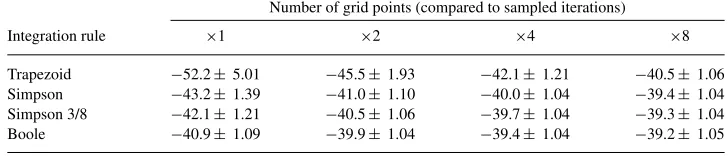
As noted by Friel, Hurn, and Wyse (2014), we can use more sophisticated numerical integration strategies to reduce the path sampling estimator bias. In the case of SMC, it is especially straightforward to estimate the required expectations at arbitrary α and so higher order integration can be used cheaply. Numerical integrations that make use of a finer mesh{α_t}T

t₌0than{αt}Tt₌0can be easily implemented. Due to the possible instability

be more appealing in some applications. A demonstration of the bias reduction effect is provided in Section4.2.

3.3.2 Adaptive Specification of Distributions. As the importance weights at time t

depend only upon the sample at time t−1, it is relatively straightforward to consider sample-dependent, adaptive specification of the sequence of distributions (typically by choosing the value of a parameter, such asαt =α(t /Tk) in the settings of SMC2 and

SMC3, based upon the current sample). Jasra et al. (2010) proposed such a method based on controlling the rate at which the effective sample size (ESS; Kong, Liu, and Wong

1994) falls. With little computation cost, this provides an automatic method of specifying a tempering schedule in such a way that the ESS decays in a regular fashion. Sch¨afer and Chopin (2013, Algorithm 2) used a similar technique but by moving the particle system only when it resamples they are in a setting equivalent to resampling at every timestep (with longer time steps, followed by multiple applications of the MCMC kernel) in our formulation. We advocate resampling adaptively only when the ESS is smaller than a preset threshold, and here we propose a more general adaptive scheme for the selection of the sequence of distributions that has better properties when adaptive resampling is employed. The ESS was designed to assess the loss of efficiency arising from the use of a simple weighted sample (rather than a simple random sample from the distribution of interest) in the computation of expectations. It is obtained by considering a sample approximation of a low-order Taylor expansion of the variance of the importance sampling estimator of an arbitrary test function to that of the simple Monte Carlo estimator; the test function vanishes from the expression as a consequence of this expansion.

In our context, allowingW_t(₋i)₁to denote thenormalized weightsof particleiat the end of timet−1, andwt(i)to denote theunnormalizedincremental weights of particleiduring

iterationt, the ESS calculated using the current weight of each particle is simply

ESSt = ⎡ ⎣ N

j=1

W_t(₋j)₁w(_tj)

N

k=1W

(k)

t−1w (k)

t 2⎤

⎦

−1

=

N

j=1W

(j)

t−1w (j)

t 2

N k₌1

W_t(₋k)₁2wt(k)

2. (3.15)

It is clearly appropriate to use this quantity (which corresponds to the coefficient of variation of the current normalized importance weights) to assess weight degeneracy and to make decisions about appropriate resampling times (see Del Moral, Doucet, and Jasra2012) but it is rather less apparent that it is the correct quantity to consider when adaptively specifying a sequence of distributions in an SMC sampler.

The ESS of the current sample weights tells us about the accumulated mismatch between proposal and target distributions (on an extended space including the full trajectory of the sample paths) since the last resampling time. Fixing either the relative or absolute reduction in ESS between successive distributions doesnotlead to a common discrepancy between successive distributions unless resampling is conducted after every iteration as will be demonstrated below.

When specifying a sequence of distributions it is natural to aim for a similar discrepancy between each pair of successive distributions. The natural question to ask is consequently, how large can we makeαt−αt₋1 while ensuring thatπt remains sufficiently similar to

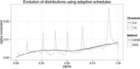
Figure 1. A typical plot of αt−αt−1 againstαt (for a Gaussian mixture model example using the SMC2 algorithm; see the supplementary material). All four samplers use roughly the same number of distributions.

sampling proposalπt−1would be for the estimation of expectations underπtand a natural

way to measure this is via the sample approximation of a Taylor expansion of the relative variance of such an estimator exactly as in the ESS .

Such a procedure (see the supplementary material for its derivation) leads us to a quantity that we have termed theconditionalESS (CESS):

CESSt = ⎡ ⎣ N

j=1

N W_t(₋j)₁

w(tj) N

k=1N W

(k)

t−1w (k)

t 2⎤

⎦

−1

= N

N

j=1W

(j)

t−1w (j)

t 2

N

k=1W

(k)

t−1

w(tk)

2 , (3.16)

which is equal to the ESS only when resampling is conducted during every iteration. The bracketed term coincides with a sample approximation (using the actual sample that is properly weighted to targetπt−1) of the expected sum of the unnormalized weights squared

divided by the square of a sample approximation of the expected sum of unnormalized weights when considering sampling from πt−1 and targeting πt by simple importance

sampling.

Figure 1shows the variation ofαt−αt−1 withαt when fixed reductions in ESS and

CESS are used to specify the sequence of distributions both when resampling is conducted during every iteration (or equivalently, when the ESS/Nfalls below a threshold of 1.0) and when resampling is conducted only when the ESS/N falls below a threshold of 0.5. As is demonstrated in Section4the CESS -based scheme leads to a reduction in estimator variance of around 20% relative to a manually tuned (quadratic; see the supplementary material) schedule while the ESS-based strategy provides little improvement over the linear case unless resampling is conducted during every iteration.

In addition to providing a significantly better performance at essentially no cost, the use of the CESS emphasizes the purpose of the adaptive specification of the sequence of distributions: to produce a sequence in which the difference between each successive pair is the same (when using the CESS one is seeking to ensure that the variance of the importance weights one would arrive at if usingπt−1as a proposal forπtis constant).

3.3.3 Adaptive Specification of Proposals. The SMC sampler is remarkably robust to the mixing speed of MCMC kernels employed (see the empirical study below). However, as with any sampling algorithms, faster mixing does not harm performance and in some cases will considerably improve it. For random walk Metropolis kernels, the mixing speed depends upon the proposalscale.

We adopt an approach similar to Jasra et al. (2010) who used sample covariance estimates to inform the proposal covariance for the next iteration. We found that such an approach generally produces satisfactory results and it is simple to implement. In difficult problems alternative approaches could be employed; one approach demonstrated by Jasra et al. (2010) is to simply employ a pair of acceptance rate thresholds and to alter the proposal scale from the simply estimated value whenever the acceptance rate falls outside those threshold values. Beskos, Jasra, and Thi´ery (2013) showed, convergence results for this kind of adaptive specification of Markov kernels.

More sophisticated proposal strategies could undoubtedly improve performance further and their use warrants investigation. One appealing approach is using the Metropolis adjusted Langevin algorithm (MALA; see Roberts and Tweedie1996). We could use the particle approximation at time indext =n−1 to estimate the covariance matrix ofπnand

thus tune the scalehonline. As these algorithms are known to be somewhat sensitive to scaling, and we seek approaches robust enough to employ with little user intervention, we have not investigated this strategy here.

3.4 A NEAR-AUTOMATIC, GENERICALGORITHM

With the above refinements, the SMC2 algorithm can be implemented with mini-mal tuning and application-specific effort while providing robust and accurate estimates of the model evidence p(y|Mk). The geometric annealing path that connects the prior

π(θk|Mk) and the posteriorπ(θk|y, Mk) provides a smooth path for a wide range of

prob-lems. The actual annealing schedule under this scheme can be determined using the adaptive schedule as described above. Finally, we can adaptively specify the Metropolis random walk (or MALA) scales through the estimation of their scaling parameters as the sampler iter-ates. In contrast to the MCMC setting, where such adaptive algorithms will usually require a burn-in period, which will not be used for further estimation, in SMC, the variance and covariance estimates come at almost no cost, as all the samples will later be used for marginal likelihood estimation. Additionally, adaptation within SMC does not require separate theoretical justification—something that can significantly complicate the develop-ment of adaptive schemes in the MCMC setting. We outline the adaptive form of SMC2 in Algorithm 4.

As laid out above, the algorithm requires minimal tuning. Its robustness, accuracy, and efficiency will be shown empirically in Section4. Automating SMC1 is less straightforward as the between model moves still require effort to design and implement. In SMC3, the specification of the sequences between posterior distributions are less generic than the geometric annealing scheme in SMC2. However, the adaptive schedule and automatic tuning of MCMC proposal scales can readily be applied.

Algorithm 4An Automatic, Generic Algorithm for Bayesian Model Comparison.

Accuracy control

Set constant CESSI_{∈(0,1), using a small pilot simulation if necessary.}

Initialization:Sett←0.

Perform theInitializationstep as in Algorithm2

Iteration:Sett←t+1

Step size selection

Use a binary search to findαI_{such that CESSα}

I =CESSI

Setαt ←αIifαI≤1, otherwise setαt ←1

Proposal scale calibration

Computing the importance sampling estimates of first two moments ofparameters. Set the proposal scale of the Markov proposalKtwith the estimated parameter variances. Perform theIterationstep as in Algorithm2with the foundαtand proposal scales.

RepeattheIterationstepuntilαt=1 then setT =t.

data or model settings, in the sense that these inputs do not need to be done on a per model or per dataset basis. We believe this framework presented here is at least a good foundation for building automatic model comparison procedures for many application areas.

Although further enhancements and refinements are clearly possible, we focus in the remainder of this article on this simple, generic algorithm that can be easily implemented in any application and has proved sufficiently powerful to provide good estimation in the examples we have encountered thus far.

4. ILLUSTRATIVE APPLICATIONS

A classical Gaussian mixture model (GMM) as formulated in Del Moral, Doucet, and Jasra (2006b) was first used to compare all three SMC algorithms with RJMCMC, AIS, and PMCMC. The details of model setting and results are in the supplementary material. It was found that all five algorithms agree on the results while the performance in terms of Monte Carlo variance varies considerably. We reached the conclusion that the SMC2 algorithm with adaptive strategies is the most promising among the SMC strategies, considering ease of implementation, performance, and generality. Also, while it has been suggested that AIS might perform similarly to SMC for the estimation of normalizing constants, the GMM example shows that resampling can have a beneficial effect on the variance allowing SMC to outperform AIS in practice.

In this section, two realistic examples, a nonlinear ordinary differential equation (ODE) model and a positron emission tomography compartmental model are used to study the performance and robustness of algorithm SMC2 compared to AIS and PMCMC. Various configurations of the algorithms are considered including both sequential and parallelized implementations.

The C++ implementations, which make use of the vSMC library of Zhou (2013), of all examples can be found athttps://github.com/zhouyan/vSMC.

4.1 NONLINEARORDINARYDIFFERENTIALEQUATIONS

Girolami (2009), is known as the Goodwin model. The ODE system, for anm-component model, is

dX1(t)

dt =

a1

1+a2Xm(t)ρ

−αX1(t)

dXi(t)

dt =ki−1Xi−1(t)−αXi(t) i=2, . . . , m Xi(0)=0 i=1, . . . , m.

The parameters{α, a₁, a₂, k_1:m−1}have common prior distributionG(0.1,0.1). Under this

setting,X1:m(t) can exhibit either unstable oscillation or a constant steady state. The data

are simulated form= {3,5}at equally spaced time points from 0 to 60, with time step 0.5. The last 80 data points of (X1(t), X2(t)) are used for inference. Normally distributed noise

with standard deviationσ =0.2 is added to the simulated data. Following Calderhead and Girolami (2009), the variance of the additive measurement error is assumed to be known. Therefore, the posterior distribution hasm+2 parameters for anm-component model.

As shown by Calderhead and Girolami (2009), whenρ >8, due to the possible instability of the ODE system, the posterior can have a considerable number of local modes. In this example, we setρ=10. Also, as the solution to the ODE system is somewhat unstable, slightly different data can result in very different posterior distributions.

4.1.1 Results. We compare results from the SMC2 and PMCMC algorithms. For the SMC implementation, 1000 particles and 500 iterations were used, with the distributions specified by Equation (3.9), withα(t /T)=(t /T)5_{, or via the completely adaptive}

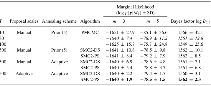
specifi-cation. For the PMCMC algorithm, 50,000 iterations are performed for burn-in and another 10,000 iterations are used for inference. The same tempering as was used for SMC is used here. Note that, in a sequential implementation of PMCMC, with each iteration updating one local chain and attempting a global exchange, the computational cost of after burn-in iterations is roughly the same as the entire SMC algorithm. In addition, changingTwithin the range of the number of cores available does not substantially change the computational cost of a generic parallel implementation of the PMCMC algorithm, with each iteration up-dating all local chains concurrently. We compare results fromT =10,30,100 for PMCMC andT =500 (or close to this number when the distributions are specified adaptively) for SMC. The results for data generated from the simple model (m=3) and complex model (m=5), summarizing variability among 100 runs of each algorithm, are shown in Tables2

and3, respectively.

As shown in both cases, the number of distributions can affect the performance of PMCMC algorithms considerably. When using 10 distributions, large bias from numerical integration for path sampling estimator was observed, as expected. With 30 distributions, the performance is comparable to the SMC2 sampler, though some bias is still observable. With 100 distributions, there is a much larger variance because, with more chains, the information travels more slowly from rapidly mixing chains to slowly mixing ones and consequently the mixing of the overall system is inhibited.

Table 2. Results for nonlinear ODE models with data generated from simple model.Italic: Minimum variance for particular algorithm.Bold: Minimum variance among samplers

Marginal likelihood (logp(y|Mk)±SD)

T Proposal scales Annealing scheme Algorithm m=3 m=5 Bayes factor logB3,5

10 Manual Prior (5) PMCMC −109.7±3.2 −120.3± 2.5 10.6± 3.8 30 −105.0±1.2 −116.1± 2.2 11.2± 2.5

100 −134.7±7.9 −144.1± 6.2 9.4± 11.2

500 Manual Prior (5) SMC2-DS −104.6±2.0 −112.7± 1.8 8.1± 2.8 SMC2-PS −104.5±1.8 −112.7± 1.5 8.2± 2.5 500 Manual Adaptive SMC2-DS −104.5±1.1 −112.7± 1.1 8.1± 1.6 SMC2-PS −104.6±1.0 −112.8± 1.0 8.2± 1.5 500 Adaptive Adaptive SMC2-DS −104.5±0.5 −112.7± 0.4 8.1± 0.8 SMC2-PS −104.6±0.4 −112.8± 0.3 8.1± 0.6

scaling were fully automatic, and significantly better for the data generated from simple model. In fact, the completely adaptive strategy was the most successful.

It can be seen that in contrast to the PMCMC algorithm, the SMC algorithm can increase the number of the distributions to reduce the bias of the numerical integration for the path sampling estimator without increasing the Monte Carlo variance.

4.2 POSITRONEMISSIONTOMOGRAPHYCOMPARTMENTALMODEL

It is now interesting to compare the proposed algorithm with other state-of-art algorithms using a realistic example.

Positron emission tomography (PET) is a technique used for studying the brain in vivo, most typically when investigating metabolism or neuro-chemical concentrations in either normal or patient groups. Given the nature and number of observations typically recorded in time, PET data are usually modeled with linear differential equation systems. For an overview of PET compartmental models, see Gunn et al. (2002). Given data (y₁, . . . , yn)T,

Table 3. Results for nonlinear ODE models with data generated from complex model.Italic: Minimum variance for particular algorithm.Bold: Minimum variance among samplers

Marginal likelihood (logp(y|Mk)±SD)

T Proposal scales Annealing scheme Algorithm m=3 m=5 Bayes factor logB5,3

10 Manual Prior (5) PMCMC −1651±27.9 −85.1±36.6 1566± 42.1

30 −1640±7.4 −78.9± 11.2 1561± 12.8

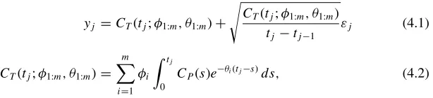
Figure 2. Estimates ofVD from a single PET scan as found using SMC2. The data show that the volume of distribution exhibits substantial spatial variation. Note that each pixel in the image represents an estimate from an individual time series. There are approximately 250,000 of them and each requires a Monte Carlo simulation to select a model.

anm-compartmental model has generative form:

yj =CT(tj;φ1:m, θ1:m)+

CT(tj;φ1:m, θ1:m)

tj −tj−1

εj (4.1)

CT(tj;φ1:m, θ1:m)= m

i=1

φi tj

0

CP(s)e−θi(tj−s)ds, (4.2)

wheretj is the measurement time ofyj,εjis additive measurement error and input function

CPis (treated as) known. The parametersφ1, θ1, . . . , φm, θmcharacterize the model

dynam-ics. See Zhou, Aston, and Johansen (2013) for applications of Bayesian model comparison for this class of models and details of the specification of the measurement error. In the simulation results below,εj are independently and identically distributed according to a

zero mean Normal distribution of unknown variance,σ2_{, which was included in the vector}

of model parameters.

Real neuroscience datasets involve a very large number of time series (∼200,000 per brain), which are typically somewhat heterogenous. Figure2 shows estimates of VD = m

j=1φj/θj from a typical PET scan (generated using SMC2 as will be discussed later).

Robustness is therefore especially important. An application-specific MCMC algorithm was developed for this problem in Zhou, Aston, and Johansen (2013). A significant amount of tuning of the algorithms was required to obtain good results. The results shown in Figure2are very close to those of Zhou, Aston, and Johansen (2013) but, as is shown later, they were obtained with almost no manual tuning effort and at similar computational cost.

For SMC and PMCMC algorithms, the requirement of robustness means that the al-gorithm must be able to calibrate itself automatically to different data (and thus different posterior surfaces). A sequence of distributions that performs well for one time series may not perform even adequately for another series. Specification of proposal scales that pro-duces fast-mixing kernels for one data series may lead to slow mixing for another. In the following experiment, we will use a single simulated time series, and choose schedules that performs both well and poorly for this particular time series. The objective is to see if the algorithm can recover from a relatively poorly specified schedule and obtain reasonably accurate results.

its relatively small number of chains, PMCMC can be parallelized completely (and often cannot fully use the hardware capability if a na¨ıve approach to parallelization is taken; while we appreciate that more sophisticated parallelization strategies are possible, these depend intrinsically upon the model under investigation and the hardware employed and given our focus on automatic and general algorithms, we do not consider such strategies here). The PMCMC algorithm under this setting is implemented such that each chain is updated at each iteration. Further, for the SMC algorithms, we consider two cases. In the first, we can parallelize the algorithm completely (in the sense that each core has a single particle associated with it). In this setting, we use a relatively small number of particles and a larger number of time steps. In the second, we need a few passes to process a large number of particles at each time step, and accordingly we use fewer time steps to maintain the same total computation time. These two settings allow us to investigate the trade-off between the number of particles and time steps. In both implementations, we consider three schedules,

α(t /T)=t /T (linear), α(t /T)=(t /T)5 _{(prior), and α(t /T)=1−(1−t /T)}5

(poste-rior). In addition, the adaptive schedule based upon CESS is also implemented for the SMC2 algorithm.

Results from 100 replicate runs of the two algorithms under various regimes can be found in Tables 4 and5 for the marginal likelihood and Bayes factor estimates, respectively. The SMC algorithms consistently outperforms the PMCMC algorithms in the parallel settings. The Monte Carlo SD of SMC algorithms is typically of the order of one-fifth of the corresponding estimates from PMCMC in most scenarios. In some settings with the smaller number of samples, the two algorithms can be comparable. Also at the lowest computational costs, the samplers with more time steps and fewer particles outperform those with the converse configuration by a fairly large margin in terms of estimator variance. It shows that with limited resources, ensuring the similarity of consecutive distributions, and thus good mixing, can be more beneficial than a larger number of particles. However, when the computational budget is increased, the difference becomes negligible. The robustness of SMC to the change of schedules is again apparent.

It can also be seen that increasing the number of distributions not only reduces the path sampling estimator bias (as seen in the previous example), but also reduces the variances considerably given the same number of particles. On the other hand, increasing the number particles can only reduce the variance of the estimates, in accordance with the central limit theorem; see Del Moral, Doucet, and Jasra (2006b) for the standard estimator and extensions for the path sampling estimator, Proposition 1 in the supplementary material. (As the bias arises from numerical integration approximation of the path sampling estimator.)

Effects of Adaptive Schedule.A set of samplers with adaptive schedules are also used. Due to the nature of the schedule, it cannot be controlled to have exactly the same number of time steps as nonadaptive procedures. However, the CESS was controlled such that the average number of time steps are comparable with the fixed schedules and in most cases slightly less than the fixed numbers.

Table 4. Marginal likelihood estimates of two component PET model.T: Number of distributions in SMC and number of iterations used for inference in PMCMC.N: Number of particles in SMC and number chains in PMCMC. The PMCMC and SMC withN=192 are completelyN-way parallelized. SMC withN=960 are N/5-way parallelized.Italic: Minimum variance for the same computational cost and the same proposal scales and annealing schemes.Bold: Minimum variance for the same computational cost and all proposal scales and annealing schemes

Proposal scales Manual Adaptive

Annealing scheme Prior (5) Posterior (5) Adaptive

T N Algorithm Marginal likelihood estimates (logp(y|Mk)±SD)

500 30 PMCMC −39.1±0.56 −926.8±376.99

500 192 SMC2-DS −39.2±0.25 −39.7±1.06 −39.2± 0.18 −39.1± 0.12

SMC2-PS −39.2±0.25 −91.3±21.69 −39.2± 0.18 −39.1± 0.13 100 960 SMC2-DS −39.3±0.36 −40.6±1.41 −39.2± 0.31 −39.2± 0.19 SMC2-PS −39.3±0.35 302.1±46.29 −39.3± 0.31 −39.2± 0.18 5000 30 PMCMC −39.3±0.21 −917.6±129.54

5000 192 SMC2-DS −39.2±0.09 −39.2±0.20 −39.2± 0.08 −39.1± 0.04 SMC2-PS −39.2±0.09 −43.8±2.13 −39.2± 0.08 −39.1± 0.04 1000 960 SMC2-DS −39.2±0.08 −39.2±0.31 −39.2± 0.07 −39.2± 0.03

SMC2-PS −39.2±0.08 −65.7±5.54 −39.2± 0.07 −39.2± 0.03

example, the bias of path sampling estimates are much more sensitive to the schedules than the previous Gaussian mixture model example. A vanilla linear schedule does not provide a low bias estimator at all even when the number of distributions is increased to a considerably larger number. The prior schedule though provides a nearly unbiased estimator, there is no clear theoretical evidence showing that this shall work for other situations. The adaptive schedule, without any manual calibration, can provide a nearly unbiased estimator, even when path-sampling is employed, in addition to potential variance reduction.

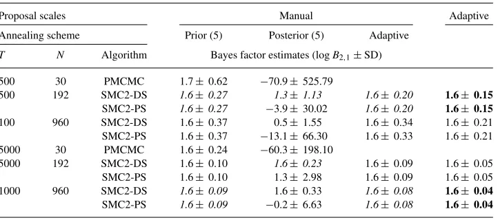
Table 5. Bayes factorB2,1estimates of two component PET model.T: Number of distributions in SMC and

number of iterations used for inference in PMCMC.N: Number of particles in SMC and number chains in PMCMC. The PMCMC and SMC withN=192 are completelyN-way parallelized. SMC withN=960 are N/5-way parallelized.Italic: Minimum variance for the same computational cost and the same schedule.Bold: Minimum variance for the same computational cost and all schedules

Proposal scales Manual Adaptive

Annealing scheme Prior (5) Posterior (5) Adaptive

T N Algorithm Bayes factor estimates (logB2,1±SD)

500 30 PMCMC 1.7±0.62 −70.9± 525.79

500 192 SMC2-DS 1.6±0.27 1.3± 1.13 1.6± 0.20 1.6± 0.15

SMC2-PS 1.6±0.27 −3.9± 30.02 1.6± 0.20 1.6± 0.15

100 960 SMC2-DS 1.6±0.37 0.5± 1.55 1.6± 0.34 1.6± 0.21 SMC2-PS 1.6±0.37 −13.1± 66.30 1.6± 0.33 1.6± 0.21 5000 30 PMCMC 1.6±0.24 −60.3± 198.10

5000 192 SMC2-DS 1.6±0.10 1.6± 0.23 1.6± 0.09 1.6± 0.05 SMC2-PS 1.6±0.10 1.3± 2.98 1.6± 0.09 1.6± 0.05 1000 960 SMC2-DS 1.6±0.09 1.6± 0.33 1.6± 0.08 1.6± 0.04