Ionisation effects for laser plasma interactions by particle in cell code

(1)

University of Warwick institutional repository: http://go.warwick.ac.uk/wrap

A Thesis Submitted for the Degree of PhD at the University of Warwick

http://go.warwick.ac.uk/wrap/57465

This thesis is made available online and is protected by original copyright.

Please scroll down to view the document itself.

(2)

Ionisation Effects for Laser-Plasma Interactions by

Particle-in-Cell Code

by

Alistair Lawrence-Douglas

Thesis

Submitted to the University of Warwick

for the degree of

Doctor of Philosophy

Department of Physics

(3)

List of Tables

2.1 Empirical factors for the MBELL electron impact ionisation cross-section 77

List of Figures

1.1 Binding energy per nucleon of elements . . . 3

1.2 Sketch of a deuterium-tritium target for ICF . . . 7

1.3 ICF ignition scheme . . . 8

1.4 NIF indirect drive scheme . . . 10

1.5 Fast ignition ICF scheme . . . 11

1.6 Regions in which the laser couples to the plasma in a density ramp to critical density . . . 13

1.7 Illustration of Landau damping . . . 19

1.8 A comparison of polarisations for EM waves oblique incident upon a density ramp to critical . . . 20

1.9 Illustration of ponderomotive force . . . 21

(6)

1.11 Crossed-beam energy transfer in direct drive ICF . . . 28

1.12 Classical interpretation of tunnel ionisation . . . 32

1.13 Sketch illustrating multiphoton resonance effects . . . 34

1.14 Simplified PIC code cycle . . . 36

1.15 Leapfrog method for alternating update of position and velocity . . . . 37

1.16 Distinction between shape and weight functions and using convolution to produce weight functions from shape functions . . . 43

1.17 The checker board instability caused by E−andB−field values sharing the same nodes . . . 45

1.18 Yee grid staggering of field values . . . 46

2.1 Unphysical bump in the ADK ionisation rate near the barrier-suppression regime . . . 64

2.2 Illustrating the requirement for restricting the ionisation rate between the three different ionisation models . . . 75

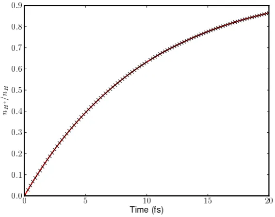
3.1 Ionisation statistics for hydrogen using a fixed rate . . . 82

3.2 Field ionisation statistics for carbon in the presence of a3×1015Wcm−2 laser compared to the results of Nuteret al. . . . 83

3.3 Accuracy scaling of field ionisation with number of superparticles per cell and time step size . . . 85

3.4 Flowchart for the partial superparticle ionisation scheme . . . 88

3.5 Illustrated ionisation of superparticles under the partial superparticle ion-isation scheme . . . 89

3.6 Comparison of the partial and whole superparticle ionisation scheme when 1−exp (−W∆t)<1/N . . . 90

3.7 Simulation of collisional ionisation results presented by Townet al. . . . 93

3.8 Ionisation-induced defocussing simulations . . . 96

3.9 Plasma mirror sharpening of a laser pulse profile . . . 97

3.10 Pulse profile for the Astra Gemini laser at the Central Laser Facility . . 98

3.11 Comparison of reflection off of a hydrogen plasma mirror in cases

(7)

3.12 Hydrogen plasma mirror switch-on time for simulations including

combi-nations of collisions, field ionisation and collisional ionisation . . . 101

3.13 Glass plasma mirror switch-on time for simulations including

combina-tions of collisions, field ionisation and collisional ionisation . . . 103

3.14 Glass plasma mirror switch-on time for field ionisation including cold

reflectivity of the neutral material . . . 106

3.15 Demonstration of differing absorption for s- and p-polarised incident laser

pulses obliquely incident upon a hydrogen plasma mirror . . . 107

3.16 Illustration of laser wakefield formation . . . 109

3.17 Electron acceleration by wavebreaking of an electron plasma wave . . . 110

3.18 Summary of laser wakefield acceleration . . . 111

3.19 Simulation of laser wakefield acceleration in hydrogen gas . . . 113

3.20 Simulation of ionisation injection by nitrogen dopant in a helium gas,

based upon experiment by McGuffeyet al. . . . 116 4.1 Simulation results demonstrating curvature of the relativistically

cor-rected quarter critical surface in plasma due to relativistically intense

incident laser . . . 123

4.2 Simulation for laser filamentation in a neutral hydrogen density ramp . 126

4.3 Relativistically corrected quarter critical surface from simulation for laser

filamentation in a neutral plastic density ramp . . . 127

4.4 Position of C5+and C6+ions and laser filaments from simulation of laser filamentation in a neutral plastic density ramp . . . 128

4.5 Simulation of laser filamentation in a neutral argon density ramp

demon-strating relativistically corrected quarter critical surface flattening . . . . 129

4.6 Position of Ar9+ through to Ar14+ions from simulation of laser filamen-tation in a neutral argon density ramp . . . 130

4.7 Simulations demonstrating suppression of SRS backscatter-induced

(8)

Acknowledgments

Firstly I would like to thank my supervisor Prof. Tony Arber for his insight and guidance

throughout this study. I would also like to thank the EPSRC for the HEC studentship

that made undertaking this Ph.D. possible. I would like to acknowledge Dr. Christopher

Brady for providing helpful advice on numerous occasions and Dr. Keith Bennett for

suffering the barrage of bug reports. The kind support from my friends and family

has been invaluable, I would especially like to thank Siobhan Riley for the constant

encouragement and the constant supply of tea. Finally I would like to mention my pet

cat, Kupo Nut, for keeping me company during the later nights writing and who sadly

(9)

Declarations

This thesis is my own work except where based upon collaborative research, in which

case the nature and extent of my contribution has been indicated at the beginning

of the relevant chapters. Some of the algorithms and results within this thesis have

been published during the course of this Ph.D. or are otherwise awaiting publication. In

particular, a condensed description of the field ionisation module and the results for laser

filamentation in ionising hydrogen and plastic are included in Physics of Plasmas in June

2012, a collaborative publication with C.S. Brady and T.D. Arber at the University of

Warwick [1]. In addition a description of the field and collisional ionisation module, the

partial superparticle ionisation scheme, and the results for laser wakefield acceleration

are soon to be submitted for publication in the Journal for Computational Physics. I

(10)

Abstract

(11)

Abbreviations

ADK - Ammosov-Delone-Krainov

BSI - Barrier-Suppression Ionisation

CDF - Cumulative Distribution Function

DPM - Double Plasma Mirror

EM - Electromagnetic

EP - Electron Plasma

EPOCH - Extendable PIC Open Collaboration

FDTD - Finite Difference Time Domain

FWHM - Full-Width at Half Maximum

IA - Ion Acoustic

ICF - Inertial Confinement Fusion

LPCR - Laser Pulse Contrast Ratio

(12)

MCF - Magnetic Confinement Fusion

MHD - Magnetohydrodynamics

NIF - National Ignition Facility

PDI - Plasma Decay Instability

PSC - Plasma Simulation Code

PWFA - Plasma Wakefield Acceleration

QED - Quantum Electron Dynamics

RCQCS - Relativistically Corrected Quarter Critical Surface

SBS - Stimulated Brillioun Scattering

SRS - Stimulated Raman Scattering

TPDI - Two-Plasmon Decay Instability

UHI - Ultra High Intensity

(13)

Chapter 1

Introduction

Laser-plasma interaction is a uniquely diverse area of physics in which the time-scales,

densities, and energies involved vary over such a range that even quantum

electrody-namics has become involved in recent study [2]. With such complexity it comes as no

surprise that some of the physical phenomena involved are analytically insoluble. In

these cases it is necessary to turn to numerics via computation to seek approximate

solutions. Computational plasma physics is therefore a rich and active area of study,

and multiple methods exist for plasma modelling such as large scale fluid

magnetohy-drodynamic codes [3] to full kinetic simulations using Fokker-Planck equations [4].

The process by which neutral material becomes plasma in the field of an intense

laser is one such interesting area of physics for which analytical methods may only be

applied for the simplest linear systems, and usually only for hydrogen. Ionisation occurs

both due to the strong electric field of a laser, and also due to particle collisions.

Lo-cally the ionised particles then influence the electric field or cause further ionisation via

collision, and it is easy to see how the situation can become very non-linear.

Despite the fact that ionisation occurs on atomic time-scales it has still been

demonstrated to produce significant consequences in laser-plasma interactions over much

longer time-scales [5, 6]. Even the short time-scale behaviour is important when viewed

in the context of plasma mirror, which depend on a fast sharp switch-on time [7]. It is

also anticipated that ionisation will prove to be a significant consideration in the field

(14)

Particle-in-cell (PIC) codes are a very intuitive set of kinetic simulations for which

charges are moved in a discretised spatial grid under the influence of their self-consistent

electromagnetic field [9]. PIC is possibly the most widely applicable plasma simulation

method, having been used to model the small scale laser-plasma interactions [10] and

also much larger scale phenomena such as magnetic reconnection [11]. For such

flexibil-ity there is a price to pay; PIC is very computationally expensive compared to an MHD

code using approximated transport coefficients. In the 60s this might have been reason

enough to overlook PIC for anything beyond one-dimensional electrostatics but in recent

decades computing has advanced to a point that relatively complex 2D simulations are

viable on a standard desktop computer. PIC is in essence an old idea which is becoming

more relevant over time.

This project concerns itself with the Extendable PIC Open Collaboration (EPOCH),

a PIC code originally developed at the University of Warwick. Based on a pre-existing

PIC algorithm, Hartmut Ruhl’s PSC code [12], EPOCH is an established relativistic fully

electromagnetic PIC code developed within the UK community and is available freely

to all UK based academics. EPOCH comes in 1D, 2D and 3D versions operating on

multiple processors for high end computing applications and is designed specifically to

be readily extensible to include new physics. This makes it an ideal candidate for the

inclusion and exploration of ionisation effects.

We will first seek to motivate the study of ionisation via computation in the

context of one of the more exciting problems in laser-plasma physics; fusion power by

laser confinement and ignition. The fundamental laser-plasma interactions will be

ex-plored in this context and theory of ionisation in an intense laser field will be outlined.

Finally particle-in-cell codes will be described in depth including the specific method for

resolving Maxwell’s equations on a discretised grid; the finite-difference-time-domain.

The following four chapters will go on to describe the implementation of ionisation in

EPOCH, validating the ionisation module, ionisation effects in the parametric

(15)

[image:15.595.147.495.114.331.2]

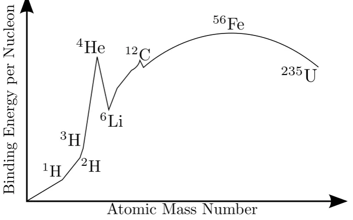
Figure 1.1: Sketch showing binding energy per nucleon against atomic mass number (arbitrary units).

1.1 Fusion

Fusion power represents a major goal for science in today’s social and economic climate,

in which our dependence on fossil fuels is increasing whilst our supplies are dwindling.

Energy is released from fusion reactions when two nuclei collide and combine into a

heavier element with a greater binding energy per nucleon. In fact our own Sun is

primarily fuelled by the fusion of hydrogen isotopes. In fusion the mass of the products

is smaller than the the rest mass of the reactants and the amount of energy released in

this reaction can be found from thismass defect using the famous equation in physics;

E=mc2. This mass defect was first noted in the 1920s by Aston and the observation that this was how the Sun burned followed shortly thereafter by Eddington.

A demonstration of nuclear fusion followed somewhat explosively in 1951 with

the use of fusion to enhance the fission reaction in a hydrogen bomb. However it

has proven a far greater challenge to science to produce nuclear fusion in a controlled

fashion that would be more applicable to a continuous power generation scheme. The

difficultly arises from the activation energy required for nuclear fusion; since the nuclei

(16)

is one of the reasons that research has focussed almost exclusively upon fusing two

isotopes of hydrogen, since a hydrogen nucleus has the lowest charge of any element

and therefore smallest Coulomb barrier to overcome. Another reason is that the fusion

reactions between hydrogen isotopes produce helium which has an anomalously large

binding energy per nucleon as demonstrated in Fig. 1.1, therefore the energy released

per reaction is amongst the highest.

A critical point to realise is that the difficulty of controlled fusion is actually

only anindirect consequence of the activation energy for the fusion reaction. It can be shown that the kinetic energy of the nuclei at which the reaction rate is maximised is

∼100keV; current designs intend fusion reactors to operate at∼10keV but even heated up to these conditions the hydrogen isotopes will be in a hot plasma state [13]. This

fact alone has driven much research in the field of plasma physics because plasmas have

highly complex dynamics that make them difficult to contain. In the Sun the plasma

confinement is achieved through gravity but on Earth we must settle for other methods; attempts to confine a plasma via application of magnetic fields started as early as 1938

before demonstration of the fusion bomb.

To continue exploring the containment of a fusion plasma it is important to

discuss what we mean by confinement. Whilst it would be ideal if we could confine a

fusion plasma indefinitely it can be acceptable for the plasma to be confined until we

have gotten more energy out of the reactions than we spent heating up the reactants.

However in general the goal is for the fusion process to generate enough heat that the

plasma heating is primarily driven by the fusion reactions themselves, a condition known

asignition. To derive these conditions we explore them in the context of a deuterium-tritium fusion reaction. This has the greatest achievable reaction rate of all the isotopes

of hydrogen, whilst deuterium itself is naturally abundant and tritium is readily produced

in situ. The reaction can be given as,

2

1D+31T→24He+10n+ 17.6MeV (1.1)

The energy released in the reaction is divided between the neutron particle

(17)

vol-ume of the D-T reaction can be written asnDnThσviwherenD andnT are the number density of deuterium and tritium respectively,σ is the cross section for D-T fusion, and

v is the mean velocity of the nuclei. For this reaction we assume that deuterium and tritium are therefore mixed in equal densities. We also assume quasi-neutrality such that

nD +nT =ne =n. From this we can write the total power produced in fusion within

volumeV,

Pfusion =

1 4n

2_h_σv_i

DTEfusV (1.2)

To consider the power required to heat the plasma Pheat we introduce the time taken τ for the plasma to lose energy W; we can then write the net change in energy as,

∂W ∂t =−

W

τ +Pheat (1.3)

This time τ is known as the energy confinement time and loosely describes a number of physical processes by which the plasma loses energy. We wish to find the

heating power for the break-even condition such that the heating balances the energy

loss from the plasma. Particles in the plasma have energy3_/₂_T _{where we use the plasma}

physics conventionT →kbT with kb the Boltzmann constant. Therefore the energy in

the volume of the plasma we have that for constant temperature and density,

Z

W dV =

Z

3

2nDTD+ 3

2nTTT + 3 2neTe

dV = 3nT

Z

dV = 3nT V (1.4)

For steady state we require that∂W_/_∂t_{= 0}_,

nT = 1

(18)

Substituting Eq. (1.2) into Eq. (1.5),

Pfusion

Pheat

= nhσνiDTEfusτ

12T (1.6)

Over the typical temperature range of for fusion of D-T the cross section for

the reaction given by Eq. (1.1), around 8−25keV, the cross-section can be fitted by

hσvi_DT≈1.1×10−24T2m3s−1 [14].

Pfusion

Pheat

= 1.6×10−20nT τ (1.7)

The factor ofnT τ gets referred to as the triple product[13] and is an important metric for determining the requirements of a fusion power scheme. Using Eq. (1.7) we

can find the break-even condition Pfusion =Pheat; the point at which the energy used to heat the plasma is balanced by the energy produced by the fusion reactions resulting

in no net loss (or gain) of energy [8]. The ignition condition can also be found; for

this we first assume that only alpha particles heat the plasma whilst neutrons provide

the energy output through some means [13]. This is because the alpha particles have

a very short mean free path within the plasma compared to the neutrons and are much

less likely to escape. Reviewing the kinetic energies of each particle following a D-T

fusion we see that the alpha particles carry approximately a fifth of the energy, therefore

Pfusion >5Pheat for ignition.

1.1.1 Inertial Confinement

Temperature is largely dictated by the requirements of the fusion reactions. Schemes

for fusion tend to vary only the plasma densities used and the energy confinement

time for the method. However there are vast differences in the governing physics when

deriving fusion power from gas density compared to solid density. There are two schemes

which attract the most research into the confinement of plasma; ICF, and magnetic

confinement fusion (MCF). The former operates with very high densities and short

energy confinement time, whereas the latter uses relatively low densities but a long

(19)

[image:19.595.151.495.104.305.2]

Figure 1.2: Basic sketch illustrating the general deuterium-tritium target design concept [8].

MCF seeks to shape the plasma through applied magnetic fields such that it is

effectively confined indefinitely if the fields can be sustained. Conversely ICF seeks to

create plasma so dense such that all the fusion reactions occur in a very short time

frame [15]. In this way a net energy output is produced before the plasma can overcome

its own inertia and fly apart [8]. In MCF numerous instabilities can destroy confinement

but in ICF the time-scale is smaller than that of most of these instabilities. However

this scheme suffers its own issues, as the density required is several hundred times

solid density of deuterium and tritium [8]. Achieving these densities therefore requires

compression of the fuel which in current schemes involves implosion of a

deuterium-tritium target of the form shown in Fig. 1.2. This is achieved via high powered lasers

imploding the target [8]. For this reason, ICF is possibly the most prolific laser-plasma

interaction application, with major experiments still occurring at the National Ignition

Facility (NIF) in California, US with ignition expected by 2013 [16].

The typical process for ICF is as follows; driver energy is applied through some

means to the plastic surface of the deuterium-tritium target. The plastic surface heats,

vaporises and blows off the target in a process known as ablation [8]. Conservation of momentum implies that the fuel is driven to the centre of the target which serves

(20)

Figure 1.3: Laser compresses the deuterium-tritium target, resulting in a hot spot of fuel undergoing fusion. The hot spot expands with a thermonuclear burn front. [8]

reactions oppose the compression and eventually cause the fuel to explode outwards;

the time it takes for this to occur is thedisassembly time and so this will be a function of the target radius.

The compressed sphere freely expands at the sound speedCS = p

4T_/₍_mD₊_mT₎

where mD and mT are the mass of the deuterium and tritium ions respectively. The energy confinement time is taken to be the time it takes for the volume of the sphere to

double such thatτ ≈R_/₄_C

S [8]. There can be no “breaking-even” in such a scheme as

there is no external heating; the heat required to drive the fusion must be produced by

the reactions themselves. In other words, ignition is required in the ICF scheme. Due

to the role of radius in confinement and fuel mass in the speed of expansion it is typical

to re-express the criteria for ignition in terms of the radius and the fuel densityρ=nm

as this yields the actual compressed fuel density requirement. From Eq. (1.7) and the

ignition requirement,

ρR >1.25×1021CSm

T (1.8)

An estimate for ignition and efficient burning of the D-T fuel is given by [8],

ρR≈0.3gcm−2 (1.9)

The compression and ignition of the D-T fuel are two distinct stages in ICF

(21)

to simultaneously compress and heat all of the fuel to the required fusion conditions,

indeed this method is known as volume ignition and was initially sought in the 1970s [8]. However it is energetically more expensive to heat rather than compress fuel and

also to compress hot rather than cold fuel. As such the driver energy requirements were

estimated at ∼60MJ [17] which is unfeasible with today’s laser technology; the most powerful laser currently being used in the development of ICF produces 1.8MJ [8]. As

such common schemes use the hot-spot concept whereby the fuel is compressed such that fusion conditions are reached in the centre only, then a thermonuclear burn front

propagates out to the rest of the fuel as shown in Fig. 1.3. This scheme is far more

efficient than volume ignition as it avoids unnecessary heating of the fuel, and is in fact

estimated to only require∼1-2MJ driver energy [8].

1.1.2 Target Design and Indirect Drive at the National Ignition Facility

The energy requirements for hot-spot ignition whilst much smaller than that of volume

ignition still present a significant challenge to present laser technology. The laser at

the national ignition facility runs at a driver energy of 1.8MJ [18] and so in principle

should achieve ignition, but the target must be illuminated uniformly which is difficult to

achieve without a very large number of lasers. Partial illumination of the target results in

uneven implosion which can result in the loss of symmetry and drive instabilities leading

to energy or fuel loss. One such mechanism is the Rayleigh-Taylor instability [19] which

can be observed when a heavier liquid sits upon a lighter liquid; the heavier penetrates

into the lighter in a spike resulting in mixing. This can be initiated by the unsymmetrical

target implosion and in the case of ICF this would result in the ablation material mixing

with the deuterium and tritium, reducing the amount of fusion material compressed into

the core.

Even with the 192 laser banks available to shine onto the target at NIF [18],

breaks in symmetry are a concern. For this reason NIF’s primary focus is upon the

indirect drive scheme illustrated in Fig. 1.4, so called due to the laser being directed upon a gold hohlraum. This is essentially a hollow cylinder with windows at either end to allow laser light entrance. The gold efficiently absorbs and re-emits the laser

(22)

[image:22.595.153.490.108.323.2]

Figure 1.4: The indirect drive scheme proposed at NIF; the laser light is focussed upon the inside of a gold hohlraum with a deuterium tritium target contained in the centre [18]. The gold absorbs and re-emits the laser energy uniformly in the form of X-rays which provides a more even illumination of the target surface.

comes with its own drawbacks; to absorb the X-rays the target ablator must be carefully

considers with current designs either using beryllium or otherwise doping with similar

substances. This makes the ablating layer heavier which exacerbates any

Rayleigh-Taylor instabilities. Whilst these are significantly reduced by the improved symmetry

but makes the target highly sensitive to manufacturing defects; any deviation from a

perfect spherical shape must be<0.1%[8].

1.1.3 Fast Ignition

Another approach being taken to ICF design is to further reduce driver energy using

a concept known as fast ignition. The goal is to separate compression and heating such that the driver energy requirements are reduced even further, though this does

serve to increase the complexity of the scheme. The model concept for this is to use a

conventional laser to compress the fuel and then use a secondary laser to directly ignite

the core; this is illustrated in Fig. 1.5. The primary issue in this scheme is how to pulse

the laser through the corona to the dense fuel in the centre. Two primary methods exist;

(23)

Figure 1.5: Laser compresses the deuterium-tritium target without hot spot formation. Laser pulse bores to the fuel core to heat the core directly to form hotspot. The fuel then ignites as before though with significantly lower energy input. [8]

into the core in a high intensity pulse, penetrating the corona. Experiments have been

performed to this end and though the pulsing laser showed increased neutron yield, it

was not clear if this was from fusion in the core or away from it at the critical surface

where the laser energy was deposited [20]. Laser cone guiding bypasses hole-boring

issues by placing the deuterium-tritium target on the tip of a hollow gold cone such that

the tip touches the core. The laser compression is still done conventionally but then

the ignition pulse is fired into the back of the cone, this ionises the gold such that fast

(24)

1.2 Laser-Plasma Interactions

The potential for fusion by laser ignition as a new energy source provides a strong

motivator for research into the interaction of laser light with plasma. It also provides

a useful context in which to describe the physical processes by which the laser light

is absorbed as shown in Fig. 1.6. In this section we seek to illustrate some important

instabilities arising from non-linear coupling of laser energy to the plasma and to outline

the process of ionisation in the field of an intense laser as a primer to this project. The

impact of the instabilities in laser-plasma interactions upon ICF ranges from universally

detrimental to potentially exploitable in certain designs. In chapter 5 we will explore

a fundamental and detrimental instability in which the plasma couples the laser to a

backwards travelling EM wave (stimulated Raman scattering) which serves to cause

loss of symmetry and drive further instabilities [1]; this in particular is an issue for

direct drive. At the end of §.1.2.1 we will also briefly explore the effect of crossed-beam energy transfer [22] in which the energy of crossed laser crossed-beams becomes unstably

coupled via a plasma wave (stimulated Brillouin scattering) which can break symmetry

in hohlraum illumination. This would seem to be an issue isolated to indirect drive but

studies by Igumenshchev et al. [23] demonstrate its relevance to direct drive. Crossed-beam energy transfer is an interesting case where research has turned to exploiting the

instability rather than mitigating it, as the energy transfer can be used to fine tune the

symmetry of the laser beams entering the hohlraum [24, 25]. To explore laser-plasma

interactions we need to know what waves propagate in a plasma and how they interact

(25)

[image:25.595.157.482.105.330.2]

Figure 1.6: The means by which laser energy couples to the plasma is dependent on the density of the plasma. When the laser is incident upon the fusion target it will encounter a density ramp and experience different absorption processes at different densities. Most occur between the quarter critical and critical surface; the processes and the density they occur at are illustrated above. [8]

First we define the phase space distribution function f(x,v, t) which provides the number density of particles which are at position x and moving at velocity v at

time t. We can find macroscopic quantities for the plasma (density, mean velocity, pressure, heat flow, etc.) by integrating the distribution function over the phase space,

for example the density atxand timetis found simply by integratingf(x,v, t)over the velocity. This macroscopic quantities are called moments of the distribution function. The first three moments are given by [26],

n=

Z

f(x,v, t)dv

u=

R

vf(x,v, t)dv

n

P=m

Z

(v−u) (v−u)f(x,v, t)dv

(26)

Particles with positive vi (v = (vx, vy, vz)) in the phase space always move

positively in xi, similarly we define the acceleration a(x,v, t) which gives the motion in v. Assuming continuity in the phase space such that particles are neither created

or destroyed then the considering the flow of particles into and out of a volume of

the phase space, we can find the Vlasov equation which describes the time evolution of a collisionless plasma [27]. This is given below for the relativistic case where γ =

p

1 +v2

/c2 _[28],

∂f ∂t +

∂ ∂x ·

v

γf

+ ∂ ∂v·

a

γf

= 0 (1.11)

Particle motion is driven by the electromagnetic fields in the plasma, so

acceler-ationa is given by the relativistic Lorentz force a=q_/_m₍_E₊v_/_γ×_B₎_{. Using this and}

the fact that v is independent of x and (v×B)_i is independent of vi we can rewrite the Vlasov equation as [27],

∂f ∂t +

v

γ · ∂f ∂x+

q m

E+ v

γ ×B

·∂f

∂v = 0 (1.12)

For a plasma containing multiple species there will be a separate distribution

function fi(x,v, t) for each species i and therefore one Vlasov equation per species

required for a full system of equation. By taking moments of the Vlasov equation

instead of the distribution function we find that the change in density depends on the

mean velocity, and the change in velocity depends on the pressure. In fact, infinite

higher order moments can be found and each will have the next higher order moment

as a term [26]. Using this fact it is possible to build up a set of relationships between

the macroscopic quantities shown in Eq. (1.10). However it is necessary to include an

approximation for one of the higher order terms so as to have a tractable system of

equations. In this case it is typical to enforce either an isothermal or adiabatic equation

of state for the pressure term so as to neglect heat flow [8].

In the adiabatic case we neglect the heat flow by assuming it is much slower

than the process under consideration, in which case the second moment of the Vlasov

(27)

of degrees of freedom. To consider the isothermal case where we instead assume that

the heat flow occurs quickly compared to the physical process of interest, this also

requires inclusion of collisions in the Vlasov equation. In this case the temperature can

be considered constant in the plasma; under this assumption the second moment of the

Vlasov equation instead reduces to the ideal gas approximation p = nkbT [26]. The

zeroth and first moments follow without any further assumption and the use of the

isothermal or adiabatic pressure reduces P to a scalar in the velocity moment. The

following equations include Maxwell’s equations and completes thetwo-fluid model for the non-relativistic case where subscript i denotes ions of atomic numberZandedenotes electrons [26],

∂ni

∂t + ∂

∂x·(niui) = 0

∂ne ∂t +

∂

∂x·(neue) = 0

nimi

∂ui

∂t +ui· ∂ui

∂x

= neme

∂ue ∂t +ue·

∂ue ∂x

= niZe(E+ui×B)−

∂pi

∂x −nee(E+ue×B)−

∂pe ∂x

∇ ×E=−∂B

∂t ∇ ×B=µ0J+µ00 ∂E

∂t

∇ ·E= ρ

0 ∇ ·

B= 0

(1.13)

This constitutes a complete description of the evolution of a plasma where

ρ = niZe−nee and J = niZeui −neeue. Note that the form of scalar pressure p

depends upon whether the adiabatic or isothermal assumption applies. Many dispersion

relations for different waves supported by the plasma follow from these three combined

sets of equations. Here we focus on three fundamental plasma waves; electromagnetic

waves from the self-consistent Maxwell’s equations in a plasma, low frequency ion

acous-tic waves from the fluid description of the ions and higher frequency electron plasma

waves from the fluid description of the electrons.

For considering the high frequency electron motion we treat the ions as

station-ary as their motion will vstation-ary slowly compared to the electrons. We also assume an

unmagnetised plasma such that rotation in the Lorentz force is eliminated. This allows

us to proceed with a simple one-dimensional analysis to find the electron plasma waves

(28)

electrostatic. Assuming small perturbations in the electron position, we make use of a technique calledlinearisation to approximate the motion. We can always write a func-tion f(x1, x2, x3, . . .) as a sum of some constant f0 = f

x(0)₁ , x(0)₂ , x(0)₃ , . . .

and a

perturbationf˜(x1, x2, x3, . . .) =f−f0. We apply this to the 1D fluid equations for the

electrons whilst picking the isothermal pressure and the equilibrium electron densityn0e

as the constant value for the pressure and density respectively. The perturbed physical

parameters are thenne =n0e+ ˜ne,ue = ˜ue,pe=n0ekbTe+ ˜p, and E = ˜E. We then linearise the equation by noting that if the perturbations are small then the product of any perturbations can be neglected; this produces linear equations,

∂˜ne ∂t +n0e

∂u˜e

∂x = 0 n0eme ∂u˜e

∂t =−n0eeE˜− ∂p˜e

∂x (1.14)

Eliminate u˜e by differentiating the density-velocity relation and the

velocity-pressure relation with respect totandxrespectively, and also substituteE˜ with Gauss’ law noting thatn0e=Zn0i for quasi-neutrality giving ρ=−e˜ne,

∂2˜n ∂t2 +n0e

∂u˜e

∂x∂t = 0 n0eme ∂u˜e

∂x∂t =−n0ee ∂E˜ ∂x −

∂2p˜e ∂x2

∂E˜ ∂x =−

e˜ne 0

⇒ ∂2n˜

∂t2+ n0ee2 0me ˜ ne=

1 me

∂2p˜e ∂x2

(1.15)

We now seek to eliminate the pressure term. For the high frequency electron

plasma waves we assume that ω_/_k _v_e _where _v_e ₌ pkbTe/_m_e is the electron thermal

velocity withTethe temperature of the electrons [26]. Therefore we use the 1D adiabatic

pressurepe=Cn3e,

∂ ∂x

n0ekbTe+ ˜pe n0e+ ˜ne

= 0⇒3 (n0ekbTe+ ˜pe) ∂n˜e

∂x = (n0e+ ˜ne) ∂p˜e

∂x

Linearising, ∂p˜e

∂x = 3kbTe ∂˜ne

∂x ⇒ ∂2_p_˜

e

∂x2 = 3kbTe ∂2_˜_n

e ∂x2

(29)

Finally we eliminatep˜eusing the above and apply a plane wave solution such that ˜

n=Aexp (ikx−iωt) whereA is a constant and i=√−1to arrive at the dispersion relation,

∂2˜ne ∂t2 = 3

kbTe me

∂2n˜e ∂x2 −

n0ee2 0me ˜

ne⇒ ω2 = n0ee2 0me

+ 3kbTe me

k2 (1.17)

Rewriting the above result in terms of the electron thermal velocity and the

electron plasma frequencyωpe= p

nee2/me0we find the common form for the dispersion

relation of electron plasma waves [8],

ω2_EP=ω_pe2 + 3k2v2_e (1.18)

The method to find the lower frequency ion density oscillations is similar to that

for electron plasma waves Eq. (1.14). Once again we use an unmagnetised plasma and

1D analysis, so this too is an electrostatic wave. The response of the electrons to any

change in the system will be fast compared to the ion oscillations, so we can begin by

neglecting the electron inertia (me ≈0) and note that in this caseω/kve such that

an isothermal equation of state pe = nekbTe applies for the electron pressure. This

reduces the linearised velocity moment of Eq. (1.14) to,

˜

E=−kbTe n0ee

∂˜ne

∂x (1.19)

For the ion thermal velocity vi we have that ω/k vi and so the pressure is found as in Eq. (1.18). We use the results for the electric field and the ion pressure and

linearise the ion fluid equations as before to arrive at the dispersion relation [26],

∂2_n_˜

i

∂t2 + Zen0i

mi

∂E˜ ∂x =

1 mi

∂2_p_˜

i

∂x2 ⇒ ∂2_n_˜

i

∂t2 − kbTe

mi

∂2_n_˜

e ∂x2 = 3

kbTi

mi

∂2_n_˜

i

∂x2 ˜

ne≈Zn˜i⇒

∂2n˜i

∂t2 =

ZkbTe+ 3kbTi mi

∂2˜ni

∂x2

(30)

Applying the plane wave solution once more, we rewrite the dispersion relation

for ion acoustic waves in terms of theion-sound velocityvs= p

(ZkbTe+ 3kbTi)/mi,

ωIAW=±kvs (1.21)

The dispersion relation for electromagnetic waves in the plasma starts with the

same assumptions as for Langmuir waves as it is assumed ω ≥ωpe, however we must consider three dimensions. Under the perturbations used previously plusB=B˜ we have that the current density is˜J=n0ie˜ui−(n0e+n˜e)e˜ue but immobile ions gives u˜i≈0 and products of perturbations are small, therefore˜J=−n0eeu˜e. We also approximate

the plasma as being cold allowing us to neglect pressure perturbation, which reduces

the velocity moment of the Vlasov equation to simply,

∂˜ue ∂t =−

e me

˜

E+˜ue×B˜

=− e me

˜

E (1.22)

Eliminating the current density from Ampere’s law and taking our plane wave

solution for the electromagnetic wave we get,

∂˜J

∂t = n0ee2

me

˜

E⇒˜J=−n0ee 2 iωme

˜

E (1.23)

Using this and the curl of Faraday’s law to eliminateB˜ from Ampere’s law, we

assume a plasma of uniform density such that ∇

∇ ·_E˜ _{= 0} _{to find the dispersion} relation for an electromagnetic wave in the plasma [26],

∇ ×_E˜ ₌₋∂B˜

∂t =iωB˜ ⇒ ∇

∇ ·_E˜_{− ∇}2_E_˜ ₌_iω_{∇ ×}_B_˜ 1

iω∇

∇ ·_E˜_{− ∇}2_E_˜ ₌_µ

0˜J+µ00 ∂E˜

∂t =

−µ0n0ee2 iωme −

µ00iω

˜ E

⇒c2∇2E˜−c2∇

∇ ·_E˜₊ _ω2₋_ω2

pe _˜

E= 0⇒ ω2−ω_pe2 −k2c2E˜ = 0

⇒ω2 =ω_pe2 +k2c2

(31)

Figure 1.7: The energy exchange between the particles and the electrostatic wave has the effect of flattening the particle velocity distribution near the phase velocity w/k

of the wave. If this is at a downward slope in the distribution then the net effect is to increase the energy of the particles. This exaggerated illustration demonstrates the effect ofLandau damping.

Note that the EM plasma waves are the only waves capable of leaving the

plasma. Langmuir and ion acoustic waves therefore remain in the plasma and

even-tually lose their energy to damping mechanisms. Two examples of electrostatic wave

damping are collisional and Landau damping [26]. Collisional damping occurs due to

electron-ion collisions and therefore damps an electron plasma wave by thermalising the

electron oscillations. This is also a direct mechanism for the plasma to absorb laser

energy; when under an applied electric field the electrons will oscillate and if they then

collide the energy is thermalised. In this case the collisional damping is called inverse

Bremmstrahlung, so named because a photon is absorbed during scattering [8].

Landau damping does not rely on collision but instead resonance with the

elec-trostatic wave meaning that only particles with v ≈ ω_/_k _{are influenced. Qualitatively,}

particles resonant with the electrostatic wave will exchange energy with it more

effec-tively. If a particle is moving slightly faster than the resonant velocity and slows towards

it then it loses energy to the electrostatic wave. Conversely if a particle is moving slower

and approaches resonance it will gain energy. It is important to note that particles are

not drawn towards the resonant velocity, but as they oscillate in the plasma they will

periodically approach it. Therefore if there are more particles accelerating up towards

the resonant velocity than decelerating down to it during their oscillation in the plasma

then on average the particles will be gaining energy. As such the overall effect of

(32)

[image:32.595.123.522.100.360.2]

Figure 1.8: An EM wave propagates obliquely into a density ramp, its direction of propagation indicated by wave vectork. When the wave iss-polarised then the electric field always points in a direction for which the plasma density is constant. However when the wave isp-polarised, the electric field has a component in the direction of the density gradient.

velocities and the result is a flattening of the distribution near the phase velocity of the

electrostatic wave; this is illustrated in Fig. 1.7.

We now know some of the key waves that propagate in a plasma and means

by which the electrostatic waves can transfer energy to the plasma. Now we briefly

discuss some ways in which the electromagnetic wave couples into the electron motion

to seed the electrostatic waves. Resonant absorption is one such mechanism, and is a

consequence of electric field polarisation with respect to a plasma density ramp rising to

critical (Fig. 1.6) and as such is of particular relevance to ICF. When the electric field

vector is in the direction of the density gradient orp-polarised as shown in Fig. 1.8, we have that the component∇

∇ ·_E˜₆_{= 0}_{. From our formulation of the electron plasma} wave in Eq. (1.15) we can see how this can excite the electrostatic wave.

The point of strongest absorption is at the critical surface where the EM wave

(33)

[image:33.595.152.519.103.336.2]

Figure 1.9: Illustration of the effect of ponderomotive force. A charge (blue) is accel-erated through the region of higherE into the area of low E where the restoring force (red arrow) is lower. The charge is accelerated faster in the high E region than it is decelerated in the lowE region. This moves the centre of oscillation (solid black) away from the original position (dashed black).

flux for resonant absorption is abs ≈ ωLEd2/8 [26] where L is the linear length of the

density ramp, andEd is the component of the electric field driving the electron

oscilla-tion along the density gradient. Kruer also shows that the strongest absorposcilla-tion is 0.5

at an oblique incident angle of the laser of θmax ≈ arcsin h

0.8 (c_/_ωL₎1/3i

[26]. It is

im-portant to note that the region over which resonant absorption occurs is very small and

since the electric field strength varies along the density ramp the plasma experiences the

ponderomotive forcewhich serves to compress this resonant region. This results in high energy electrons near the shock in ICF which is detrimental to the early compression

[8]. Motion due to ponderomotive force is best understood as the net movement of the

centre point of oscillation for electrons in an EP wave as described in Fig. 1.9. This

effect is readily derived for an electron in a non-uniform oscillating electric field in x,

E(x, t) = E(x) sin (ωt). For the simplest case in the absence of magnetic fields the Lorentz force gives that the motion of an electron in this field will be,

me due

(34)

Now model the motion of the electrons with a net drift velocity u0e that varies

slowly and the fast oscillationsu˜e such that the particle position can be divided into the

centre of oscillationx0eand the small perturbationx˜e due to oscillation. This allows us

to Taylor expandE(x),

me d

dt(u0e+ ˜ue) =e

E(x0e) + (x−x0e)

dE(x0e) dx +. . .

sin (ωt)

≈e

E(x0e) + ˜xe

dE(x0e) dx

sin (ωt)

(1.26)

We have definedu0eto refer to the slowly varying drift, and assumedx˜eis small.

Therefore we takex0e to be a constant over the small oscillations andE x˜edE/dx,

me d˜ue

dt =eE(x0e) sin (ωt)⇒x˜e =− e meω2

E(x0e) sin (ωt)

⇒me du0e

dt =− e2 meω2

E(x0e)

dE(x0e) dx sin

2_(ωt)

(1.27)

We now time average over the a single period in the electric field oscillation to

find the force associated with the change in drift velocity,

me

due dt

= meω 2π

Z 2π ω

0

− e2

meω2

E(x0e)

dE(x0e) dx sin

2_(ωt)_dt

⇒Fdrift=−

e2 4meω2

d dxE

2_(x)

(1.28)

This force is the ponderomotive force, which Kruer gives for a plasma in

3-dimensions as [26],

Fp=− e2 4meω2∇

(35)

1.2.1 Parametric Instabilities

Parametric instabilities are a set of mechanisms by which laser energy is absorbed by the

plasma but differs from resonant absorption in that they tend to drive unstable growth

of multiple plasma waves at various frequencies. The name comes from parametric

os-cillators, a form of damped harmonic oscillation in which the parameters (e.g. damping,

frequency, forcing) can vary in time. For plasma waves given by oscillators x1 and x2

and a laser inputpumpEwe can model a 1D parametric instability by use of the general form of a parametric oscillator and a force term F(t) ∝x2E for x1 and ∝x1E for x2

to represent the coupling between the three waves. For constants C representing the strength of this coupling andγ the damping coefficient [30],

d2x1 dt2 +γ1

dx1 dt +ω

2

1x1=C1x2E (1.30)

d2x2 dt2 +γ2

dx2 dt +ω

2

2x2=C2x1E (1.31)

Where damping and forcing is neglected the termsω1 andω2 are the frequency

for the simple harmonic motion ofx1 andx2 respectively. If we take a general form for

the laser pump asE =E0cos (ω0t) we can find the frequencies at which this coupling

can occur through Fourier transform of Eq. (1.30) and Eq. (1.31). We use the notation

ˆ

x(ω) = 1_/₂_πR_x_{(t) exp (iωt)}_dt _{and that for linear equations under Fourier transform}

d_/_dt→_iω_,

ω1+iγ1ω−ω2

ˆ

x1(ω) = C1E0

2π

Z

x2cos (ω0t) exp (iωt)dt = C1E0

4π

Z

x2exp [i(ω+ω0)t]dt+

Z

x2exp [i(ω−ω0)t]dt

= C1E0

2 [ˆx2(ω+ω0) + ˆx2(ω−ω0)]

(1.32)

From this we can see thatxˆ1(ω) is coupled to oscillationsxˆ2(ω±ω0)through

(36)

ω+ω0 andω−ω0 in x2. For the latter we multiply Eq. (1.31) through by exp (iω0t)

prior to Fourier transform to produce the frequency shift,

ω2+iγ2(ω+ω0)−(ω+ω0) 2

ˆ

x2(ω+ω0) =

C2E0

2π

Z

x1cos (ω0t) exp (iωt) exp (iω0t)dt

=C2E0 2π

Z

x1exp [iω0t] exp [i(ω+ω0)t]dt+ Z

x1exp [−iω0t] exp [i(ω+ω0)t]dt

=C2E0

2 [ˆx1(ω+ 2ω0) + ˆx1(ω)]

Similarly,

ω2+iγ2(ω−ω0)−(ω−ω0) 2

ˆ

x2(ω−ω0) =

C2E0

2 [ˆx1(ω) + ˆx1(ω−2ω0)]

(1.33)

Now it can be seen that the oscillation xˆ2(ω−ω0) feeds back to the

oscilla-tion xˆ2(ω). We can find a similar relation for xˆ2(ω+ω0) by multiplying Eq. (1.31)

through byexp (−iω0t). We explore the case where damping and non-resonant terms ˆ

x1(ω±2ω0) are negligible such that the system of equations can be written,

  

ω2₋_ω2

1 C12E0

C1E0 2

C2E0

2 (ω−ω0) 2₋_ω2

2 0

C2E0

2 0 (ω+ω0)

2₋ ω₂2

      ˆ x1(ω) ˆ

x2(ω−ω0) ˆ

x2(ω+ω0)

 

= 0 (1.34)

For a non-trivial solution of Eq. (1.34) the determinant must be zero. When

oscillatorxˆ1 grows slowly we have thatω≈ω1 in which caseω02 = (ω2−ω1) (ω1+ω2)

for zero determinant. The(ω2−ω1)comes from thexˆ2(ω1−ω0)term whilst(ω2+ω1)

comes from the xˆ2(ω1+ω0). The parametric instabilities explored here involve the

laser decaying into two of the three plasma waves derived in Eq. (1.18), Eq. (1.21) and

Eq. (1.24). Therefore higher frequency pump ω0 decays into lower frequency plasma

waves ω1 and ω2; this allows us to neglect the xˆ2(ω1+ω0) term as non-resonant, in

which case we find the frequencies at which this feedback occurs as,

(37)

This is called the frequency matching condition and a similar equation can be found for the wavevector, which together describe the energy and momentum

conser-vation for the decay [30],

k0 =k1+k2 (1.36)

There are four types of decays from the incident laser into the three plasma

waves derived in this section [8]. These are given below where EM is an electromagnetic

wave, IA is an ion-acoustic wave, and EP is an electron plasma wave. Not all of these

decays can occur in 1D, but for those that can we can plot the dispersion relations

for the three plasma waves together for useful visual method to determine where these

frequency matching conditions will be met; this is demonstrated in Fig. 1.10.

• Plasma decay instability, EM→IA+EP

• Two-plasmon decay instability, EM→ EP+EP

• Stimulated Brillouin scattering, EM→EM+IA

• Stimulated Raman scattering, EM→ EM+EP

As shown in the derivation of Eq. (1.34), these mechanisms are unstable because

the three-way coupling of waves instigates a feedback effect. In the case of stimulated

Raman scattering if there is a density gradient in the direction of laser propagation then

an EP wave will be initiated by the laser field. The electron motion in the presence of

an electric field gives rise to a current density, and this is associated with a scattered

EM wave. This new EM wave interferes with the incident laser field which can cause a

gradient in the electric field. As we have seen derived in Eq. (1.28), this gradient gives

rise to a ponderomotive force which can serve to drive the electron plasma wave. Under

proper frequency and wavenumber matching conditions this feedback mechanism can

undergo unstable growth.

The strongest mode of SRS is where the new EM wave is backscattered [26];

that is to say it propagates backwards along the propagation of the incident laser. In

the context of ICF, SRS backscatter tends to cause the head of the laser to break up

(38)

[image:38.595.120.502.108.740.2]

(39)

this is explored in greater detail in Chapter 4. In other directions, random scattering of

light also has negative effects upon the symmetry in all ICF scheme; as much as 25% of

the laser energy has been observed to be scattered this way [18]. In general all of the

parametric instabilities presented here are found to be detrimental to the ICF scheme

[8]. As shown in Fig. 1.6 the instabilities occur at different points in the density ramp;

this is dictated by the frequency matching conditions. In the case of SRS, we know that

the EP wave occurs at the plasma frequency, and for the scattered EM wave to exist in

the plasma we require thatωEM> ωpe. From the matching conditions,

ω0 ≈ωEM+ωEP ⇒ω0 &2ωpe ⇒nSRS. nc

4 (1.37)

The strongest point of Raman-scattering is seen at nc/₄; the EP wave can be

observed by an increase of hot electrons and in hohlraum experiments it was found that

50% of incident light energy could be driven into these hot electrons [18]. It should be

noted that the simple analysis used in Eq. (1.34) excludes damping, but any EP and IA

waves could be damped to the point that the instability is effectively switched off. By

including damping we can find the threshold intensity that the incident laser must exceed

for the instabilities to be present. This also allows us to calculate the growth rate of the

instabilities, and it is found that that all of the parametric instabilities presented here

exhibit a γ ∼√Iλ2 _{scaling [8, 26, 30]. Stimulated Brillouin scattering (SBS) couples}

the incident laser field into both an EM and IA wave and is analogous to SRS for lower

frequency IA waves. Since in general ωIA ωEM the frequency matching condition gives,

ω0 ≈ωEM&ωpe ⇒nSBS .nc (1.38)

Since SBS can occur right up to the critical surface, the ion acoustic waves will

have the effect of pulling ions out of the fusion fuel in an ICF context [8]. However

the ion acoustic wave tends to be strongly damped unless Te Ti [26] and so the threshold intensity for the instability tends to be relatively high. The plasma decay

(40)

Figure 1.11: The fringe of the transverse intensity profile of a laser spot misses the ICF deuterium tritium target and crosses the path of a second incident laser. Energy from the second beam couples to the fringe of the first via an ion acoustic wave (induced Brillouin scattering) resulting in energy being channelled into the fringe and away from the target [23].

density fluctuation but instead this drives an EP wave. As with SRS the electric field

across a density gradient results in a ponderomotive force which may be enhanced by

the EP wave. In the case that the ion density fluctuation is caused by an IA wave we

can see how the feedback mechanism between the three waves builds up at the correct

frequencies. As with SBS we also note that ωIA ωEP therefore ω0 ≈ ωEP from the

frequency matching condition and therefore this instability occurs only at the critical

surface. This time we expect that the decay will not only extract fuel from a laser fusion

target but also potentially drive hot electrons into the fuel via the electron plasma wave

thereby damaging compression.

SBS is also the cause of one of the more useful consequences of parametric

instability, namely crossed-beam energy transfer [22, 24, 25]. As the name implies this

occurs when two incident laser beams cross within a plasma, a situation seen in the

hohlraum for indirect drive ICF. Understanding that SBS couples the incident laser to

a scattered EM and IA wave we can consider crossed-beam energy transfer as being

a special case of SBS where the scattered EM wave is another incident laser; this is

(41)

two beams must differ in frequency; an IA wave couples these crossed-beams together

and in much the same way that energy can be transferred from an incident laser into

a scattered EM wave, energy can be transferred between the two beams. This can be

detrimental to the indirect drive scheme as it can cause asymmetry in the illumination

of the hohlraum, however it can also be harnessed to aid symmetry through tuning of

the frequencies to either increase or decrease this energy transfer [24]. Crossed-beam

energy transfer is also relevant to direct drive schemes; when multiple beams shine on

the target, if a beam is wide enough for the fringes to miss the target but cut across

another beam then energy can be coupled out of the beam hitting the target and into

the beam missing the target resulting in energy loss as illustrated in Fig. 1.11 [23].

The two-plasmon (EP wave) decay instability (TPDI) also occurs due to electron

density fluctuation as with SRS. However instead of decaying into an EM wave

associ-ated with the current density from the EP wave crossing the electron density gradient,

two EP waves are seeded in such a way that the current densities from each wave cancel.

In effect there is no net current density and so no new EM wave is produced, but two

separate EP waves are driven. As with SRS frequency matching conditions indicate that

ω0≈2ωpe therefore TPDI only occurs whenn≈ncr/4 and the tendency is for TPDI to

cause bursts of hot electrons.

TPDI is a good example of how parametric instabilities also interact with each

other as well as the laser; if there are other sources of EP waves then TPDI may couple

them to the laser, producing more EP waves and more potential couplings such that a

cascade of TPDI can occur. The hot electrons produced from EP wave damping at the

quarter critical surface is extremely destructive to direct drive ICF schemes. There are

many other unexpected combinations of parametric instabilities, and actually predicting

what effect these may have in experiment can be particularly difficult. For instance, one

might expect that SBS would cause intense reflection at the critical surface preventing

energy absorption close to the fusion fuel, however it is found that SBS only occurs very

briefly [32] and therefore has almost no impact on compression or heating. Both SRS

and SBS switch-on and off rapidly due to the product waves growing to reach threshold

intensities for any other instability, and so analysing any linear instability in isolation is

(42)

experiment or numerical analysis; direct numerical solution of the Vlasov equation have

been shown to provide a detailed view of the distribution functions allowing for

mod-elling the parametric instabilities without noise even with a low particle count [33]. This

is even computationally undemanding in 1D but is expensive in 2D due to requiring

2D space and 2D velocity resulting in a 4D computational grid, it also requires

man-ual initial perturbation to produce useful results. For larger simulations particle-in-cell

simulations also excel at reproducing parametric instabilities with significantly reduced

computational cost at the expense of increased noise [9].

1.2.2 Ionisation in the Field of an Intense Laser

Although plasmas are ionised material, the process of ionisation is not typically a primary

consideration in plasma phenomena. This is often justified, as the process of ionisation

is often on a smaller timescale than is relevant to plasma waves and instabilities which

are the focus of many plasma studies. However there are some cases where ionisation is

key, for instance when the distribution of electrons produced by ionisation is important

and cannot be assumed or the timescales are small such as those relevant to

femtosec-ond laser pulses. The process by which neutral material transitions to the plasma state

can therefore be an integral part of laser-plasma interactions, and also challenging to

model correctly.

The mechanism of ionisation in the laser field differs depending on the

temper-ature, density and level of ionisation within the plasma and also the intensity of the

incident laser field. We might initially describe the ionisation process as photons

ab-sorbed by a bound electron within an atom via the photoelectric effect. However if

the electric field is strong enough we can expect the energy levels within the atom to

be shifted via the Stark effect [34] which would affect the photon energy required for

ionisation. The difficulty in modelling this is increased when considering that the field is

time-varying. In addition to this it is initially unclear how the photoelectric effect applies

when considering the energy of a photon in a typical laser; the National Ignition Facility

Ionisation effects for laser plasma interactions by particle in cell code

University of Warwick institutional repository: http://go.warwick.ac.uk/wrap

A Thesis Submitted for the Degree of PhD at the University of Warwick

http://go.warwick.ac.uk/wrap/57465

This thesis is made available online and is protected by original copyright.

Please scroll down to view the document itself.

Ionisation Effects for Laser-Plasma Interactions by

Particle-in-Cell Code

Alistair Lawrence-Douglas

Department of Physics

Contents

List of Tables

List of Figures

Acknowledgments

Declarations

Abstract

Abbreviations

Chapter 1

Introduction

1.1

Fusion

1.2

Laser-Plasma Interactions