Auction Mechanisms Toward Efficient Resource Sharing for Cloudlets in Mobile Cloud Computing

Auction Mechanisms Toward Efficient Resource

Sharing for Cloudlets in Mobile Cloud Computing

A-Long Jin, Wei Song, Ping Wang, Dusit Niyato, and Peijian Ju

Abstract—Mobile cloud computing offers an appealing paradigm to relieve the pressure of soaring data demands and augment energy efficiency for future green networks. Cloudlets can provide available resources to nearby mobile devices with lower access overhead and energy consumption. To stimulate service provisioning by cloudlets and improve resource utilization, a feasible and efficient incentive mechanism is required to charge mobile users and reward cloudlets. Although auction has been considered as a promising form for incentive, it is challenging to design an auction mechanism that holds certain desirable properties for the cloudlet scenario. Truthfulness and system efficiency are two crucial properties in addition to computational efficiency, individual rationality and budget balance. In this paper, we first propose a feasible and truthful incentive mechanism (TIM), to coordinate the resource auction between mobile devices as service users (buyers) and cloudlets as service providers (sellers). Further, TIM is extended to a more efficient design of auction (EDA). TIM guarantees strong truthfulness for both buyers and sellers, while EDA achieves a fairly high system efficiency but only satisfies strong truthfulness for sellers. We also show the difficulties for the buyers to manipulate the resource auction in EDA and the high expected utility with truthful bidding.

Index Terms—Mobile cloud computing, cloudlet, double auction, incentive design, truthfulness, efficiency.

✦

1

I

NTRODUCTION

In recent years, mobile network operators are facing unremit-ting demands for high date rates and ever-emerging new applications. While this growth leads to increasing revenue to the global mobile industry, there are rising concerns on environmental impact and high capital/operating expenditure. Meanwhile, cloud computing is achieving great success in empowering end users with rich experience by leveraging resource virtualization and sharing. The merging of cloud com-puting into the mobile domain creates the appealing paradigm of mobile cloud computing (MCC). MCC offers a promising solution not only to extend the limited capabilities of mobile devices, but also to reduce energy consumption if designed in a green manner [1].

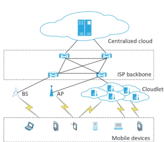
As illustrated in Fig.1, the traditional centralized cloud [2] hosts shared resources in remote data centers and acts as an agent between the original content providers and mobile devices. To access resources/services at the data centers, mo-bile devices often need to go through the backbone network. The long latency and high energy consumption can hamper the capability of the cloud to support interactive applications demanded by users. In contrast, the lightweight cloudlet [3] can balance the scale of shared resources and the access overhead. A cloudlet is a trusted, resource-rich, Internet-connected computer or a cluster of computers, which can be utilized by mobile devices via a high-speed wireless local area • A. Jin, W. Song (corresponding author), and P. Ju are with the Faculty of Computer Science, University of New Brunswick, Fredericton, Canada (emails: [email protected], [email protected], [email protected]). This research was supported in part by Natural Sciences and Engineering Research Council (NSERC) of Canada.

• P. Wang and D. Niyato are with School of Computer Engineering, Nanyang Technological University, Singapore (emails: [email protected], [email protected]).

Centralized cloud

ISP backbone

BS

Mobile devices Cloudlets AP

Fig. 1: Typical MCC architectures: Centralized cloud and cloudlets. network (WLAN). In this architecture, mobile devices function as the clients and cloudlets as the service providers. Seamless interaction between them can be more easily achieved in the cloudlet’s physical proximity with the low one-hop communi-cation latency. Due to the spatial distributions of cloudlets and their distinct capabilities or hosted resources, mobile devices have different preferences over the cloudlets. On the other hand, the cloudlets need to be incentivized to share their resources, e.g., through gaining monetary values paid by the mobile devices for using the services. As seen, there exists a trade between the mobile devices requesting the services and the cloudlets providing such services.

Auction is a popular trading form that can efficiently distribute resources of sellers to buyers in a market at com-petitive prices. Auction theory [4] is a well-researched field in economics and has been applied to other domains, e.g., radio resource management for wireless systems [5]. If the

resource trading system with buyers and sellers is viewed as an ecosystem, the auction mechanism needs to appropriately address the conflicting interests of buyers (e.g., minimizing charge for highest valuation) and sellers (e.g., maximizing reward for least cost), and internal competitions among buy-ers/sellers. The mechanism should fairly allocate the trading resources, determine the pricing, and optimize the payoff that each buyer/seller can achieve with the presence of compe-titions. As such, the buyers and sellers can be incentivized to participate in the auction and the ecosystem can reach an equilibrium. Such an auction mechanism is expected to hold certain desirable properties, such asindividual rationality,

budget balance,truthfulnessorincentive compatibility,system efficiency, andcomputational efficiency.

Individual rationality ensures that a buyeris never charged more than its bid, while aseller is paid not less than its ask. Budget balance requires that theauctioneer, which acts as an intermediate agent between buyers and sellers, hosts and runs the auction without a deficit. Truthfulness is essential to resist market manipulation and ensure auction fairness. An auction mechanism is truthful (also known as incentive compatible) if revealing the private valuation truthfully is always the weakly dominant strategy for each participant to receive an optimal utility, irrespective of what strategies other participants are taking. There are various definitions of efficiency in economics from different perspectives, among which allocative efficiency is a main type that aims to maximize social welfare, i.e., the sum of valuations of the buyers who receive their desired

commodities. In this paper, we are particularly interested in double auction, in which buyers and sellers submit to an auctioneer their bids and asks, respectively. For such bilateral trade, a mechanism is efficient if whenever a buyer’s bid is greater than the seller’s ask, the corresponding commodity is allocated to the buyer [4]. In addition to the above economic properties, computational efficiency ensures that the auction outcome is tractable with a polynomial time complexity, which is important to enable feasible implementation.

Many existing auction mechanisms cannot be directly ap-plied to the cloudlet scenario without jeopardizing certain de-sired properties. For example, the multi-round auctions studied in [6]–[8] are not suitable due to the high communication and computation overhead. For double auction, no mechanism can be efficient, truthful, individually rational, and at the same time balance the budget [4]. Considering only homoge-neous commodities, McAfee double auction [9] can achieve three desirable properties, i.e., individual rationality, budget balance, and truthfulness. The Truthful Auction Scheme for Cooperative communications (TASC) proposed in [10] extends McAfee double auction by taking into account heterogeneous trading commodities, i.e., services of relay nodes. Although TASC addresses a similar scenario, it is found that the effi-ciency of TASC can be further improved. In [11], the Vickrey-based double auction exploits the participant’s uncertainty of bids/asks of other participants to reduce manipulation and boost allocative efficiency, while enforcing budget balance and individual rationality. This mechanism can be fairly efficient and fairly truthful, but not computationally efficient.

As seen, it is impossible to simultaneously satisfy all the

aforementioned desirable properties in an auction mechanis-m. In many cases, certain properties (e.g., computational efficiency or truthfulness) have to be relaxed to trade for other properties (e.g., system efficiency). As a result, this leaves room for improving the relaxed properties. In this paper, we focus on designing feasible and efficient double auction mechanisms to stimulate cloudlets to serve nearby mobile devices. Here, a feasible auction mechanism needs to satisfy computational efficiency, individual rationality, budget balance, and truthfulness. Consequently, we have to relax the requirement for system efficiency, which is sub-optimal but sufficiently close to the optimum. First, we propose a truthful incentive mechanism (TIM), which is also computationally efficient, individually rational and budget-balanced. To further improve the system efficiency, we extend TIM to a more effi-cient design of auction (EDA), by involving randomness and bidding uncertainty. EDA maintains all desired properties of TIM except for slightly relaxed truthfulness. EDA guarantees trustfulness of sellers but it is not strongly truthful for buyers. We provide rigorous analysis regarding these properties of both mechanisms. Numerical results confirm the analysis and demonstrate their desirable properties, especially the high system efficiency achieved by EDA. It is also shown that EDA is truthful in expectation for buyers.

The remainder of this paper is structured as follows. First, we briefly review related auction mechanisms in Section 2. Then, Section 3 provides the problem formulation as a double auction and an example demonstrating the design rationale. After that, we give the design details of the proposed TIM and EDA mechanisms in Section 4 and Section 5, respectively. Numerical results are presented in Section 6, followed by conclusions in Section 7.

2

R

ELATED

W

ORK

As a promising paradigm, mobile cloud computing has at-tracted considerable research attention and efforts. There have been a number of studies addressing various aspects of MCC, such as virtual machine migration [12], service enhancement with MCC [13], and emerging applications with MCC [14,15]. However, the research on incentive design for MCC is lim-ited, although there have been many incentive mechanisms proposed for wireless cooperative communications [10], radio resource allocation [5], device-to-device communications [16], smartphone sensing [17], and smart grid [18].

In [10], Yang et al. propose a truthful double auction mechanism, TASC, to stimulate relay nodes to forward packets for other wireless nodes. TASC has two stages, namely,

Assignment and Winner-Determination & Pricing. In the as-signment stage, the auctioneer applies an asas-signment algorithm to determine the winning buyer candidates (source nodes), the winning seller candidates (relay nodes), and the mapping between these buyers and sellers. Depending on the design objective, the auctioneer can choose a different assignment al-gorithm. For example, the optimal relay assignment algorithm [19] can maximize the minimum valuation among all buyers; the maximum weighted matching algorithm [20] can maximize the total valuation; and the maximum matching algorithm can

maximize the number of successful trades (final matchings). In the winner-determination & pricing stage, TASC tightly integrates the winner determination and the pricing operation. Based on the return of the assignment stage, the auctioneer applies McAfee double auction [9] to determine the winning buyers, the winning sellers, and the corresponding clearing price and payment.

TASC overcomes the limitation of the original McAfee double auction [9] that considers only homogeneous com-modities, i.e., buyers have no preference over auction items. When TASC is used in the cloudlet scenario, it can satisfy individual rationality, budget balance, and truthfulness for the sellers. However, we use an example in Section 3.4 to illustrate that the system efficiency of TASC can be further improved.

Another closely related work in [21] addresses specifically resource sharing with MCC. In [21], cloud resources are cate-gorized into several groups (e.g., processing, storage, and com-munications). The resource allocation problem is formulated as a combinatorial auction with substitutable and complementary commodities. This combinatorial auction mechanism is not applicable for the cloudlet architecture since its key problem is the allocation of M resources of G groups in one MCC service provider toN users. In contrast, our system model with cloudlets focuses on distinct valuations of cloudlets to mobile users. Different from [21], we further consider computational efficiency and budget balance, which are also critical to an auction mechanism.

It is noted that many existing incentive mechanisms em-phasize the property of truthfulness, which prevents market manipulation and eliminates the strategic overhead of the participants. However, there are few works on double auction design to improve system efficiency. In [11], Parkes et al.

propose a Vickrey-based double auction, which can achieve individual rationality and budget balance. The assignment between buyers and sellers is determined to maximize social welfare (system efficiency), while the participant’s utility equals the incremental contribution to the overall system, i.e., the difference between the social welfare with and without the participation. However, the Vickrey-based double auction in [11] is only fairly efficient and fairly truthful. Moreover, this mechanism cannot satisfy computational efficiency.

3

P

ROBLEM

F

ORMULATION 3.1 System Model

As depicted in Fig. 1, the cloudlets offer resource pools closer to the network edge. Thus, the close proximity of cloudlets can be exploited to reduce the access overhead of mobile users in terms of energy consumption and communication latency. The resources at the cloudlets may be valued differently by the mobile users depending on various factors [22], such as computation capability, communication cost, and wireless link performance (e.g., throughput, latency, and link variation). Such valuation of a mobile user toward a cloudlet is also associated with the application demand. For instance, when a mobile user offloads a computation-intensive task, it values high a cloudlet with rich computing resources of memory and CPU capacity. In contrast, a mobile user with a real-time task

prefers a cloudlet with a short communication latency, which requires large network bandwidth and close spatial locations. As seen, the valuation of a mobile user toward a cloudlet actually takes into account the service quality that the cloudlet can provide to the user.

On the other hand, the cloudlet can be paid for sharing resources as compensation for its computation and commu-nication cost. The cost covers the cloudlet’s expenditures on acquiring computation resources (e.g., computing equipment, energy, and storage), and leasing communication facility from ISPs, mobile carriers, or network operators. Note that the cost implicitly incorporates the resource constraint of the cloudlet. Clearly, the trading between the cloudlets and the mo-bile users should meet certain requirements to benefit both the cloudlets and mobile devices. The cloudlets need to be incentivized to provide the resources, and the demands of the mobile users should be satisfied. In particular, a cloudlet cannot be paid less than its cost, while the allocated resources of the cloudlet must fulfill a mobile user’s service request. To maximize the resource utilization, the incentive mechanism should properly assign the matching between the cloudlets’ resources and the mobile users’ demands.

3.2 Auction Model

To assist the matching between mobile users and cloudlets, a trusted third party is necessary to administer the trading between them, e.g., in the form of auction. In particular, a double auction fits well the bilateral nature of this scenario. The trusted third party in a double auction is the auctioneer

between mobile users (buyers) and cloudlets (sellers). The auctioneer needs to determine the matching of winning buyers and winning sellers, the price it charges the buyers and the price it rewards the sellers.

Apparently, the auctioneer should at least run the auction without a deficit and preferably benefit from the process. Taking the dominant video streaming service as an example, we can identify some network entities that would support the auctioneer functionality. In practice, content providers often pay content delivery network (CDN) operators to deliver their content, while a CDN operator in turn pays ISPs, mobile carriers, or network operators for hosting its servers in their data centers [23]. Besides, cloudlets can offer services clos-er to network edge, thus complementing traditional CDNs with lower delivery cost and better performance. Hence, the end users need to pay the content providers for content consumption, while the content providers in turn pay CDN operators or cloudlets for content delivery. Because cloudlets when available can deliver content with lower cost and higher quality, the content providers sitting between the end users and cloudlets can have a strong motivation and suitable position to run an auctioneer server to reduce their expenditures and sustain competitiveness.

Considering m cloudlets (sellers) that provide available resources fornmobile devices (buyers), we formulate the un-derlying resource allocation problem as a single-round multi-item double auction similar to [10]. Each buyer (resp. seller) can submit its bid (resp. ask) privately to the auctioneer so that everyone has no knowledge of others.

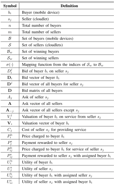
TABLE 1: Important notations.

Symbol Definition

bi Buyer (mobile device)

sj Seller (cloudlet)

n Total number of buyers

m Total number of sellers

B Set of buyers (mobile devices)

S Set of sellers (cloudlets)

Bw Set of winning buyers

Sw Set of winning sellers

σ(·) Mapping function from the indices ofSwtoBw

Dij Bid of buyerbion sellersj D_i Bid vector of buyerbi

Dj Bid vector of all buyers for sellersj D Bid matrix of all buyers

Aj Ask of sellersj A Ask vector of all sellers

A_{−j Ask vector of all sellers except}sj

Vij Valuation of buyerbion service from sellersj V_i Valuation vector of buyerbi

Cj Cost of sellersj for providing service

Pib Price charged to buyerbi

Pjs Payment rewarded to sellersj

Pijb Price charged to buyerbi for service of sellersj

Pijs Payment rewarded to sellersjwith assigned buyerbi

Uib Utility of buyerbi

Ujs Utility of sellersj

Uijb Utility of buyerbi with assigned sellersj

Uijs Utility of sellersjwith assigned buyerbi

• For each buyer bi∈ B,B={b1, b2, . . . , bn}, its bid vector

is denoted by D_{i = (D}1

i, Di2, . . . , Dmi ), where D j i is the

bid for sellersj∈ S,S ={s1, s2, . . . , sm}. The bid matrix

consisting of the bid vectors of all buyers is defined asD₌

(D_1;D_{2;. . .;}D_n).

• For all sellers in S, the ask vector is denoted by A =

(A1, A2, . . . , Am), whereAj is the ask of seller sj∈ S.

As seen, the asks of sellers do not differentiate among buyers since the sellers only aim at collecting payments for using their resources. On the other hand, the bids of buyers differ with respect to sellers as mobile devices have preferences over the cloudlets. Although the bids of buyers are private information to the sellers, the cloudlets do need to release certain information, such as their hosted resources, computation capabilities, network bandwidth and communi-cation latency, to nearby mobile users, so that the users can determine their valuations toward the cloudlets. The cloudlets, however, keep their service costs confidential. The auctioneer that holds the private information thus needs to apply security mechanisms [24] to guarantee protection of privacy.

Given B,S,D _and A_{, the auctioneer decides the winning}

buyer setBw⊆ B, the winning seller setSw⊆ S, the mapping

betweenBw andSw, i.e.,σ:{j:sj ∈ Sw} → {i:bi∈ Bw},

the pricePb

i that the winning buyerbi∈ Bw is charged, and

the paymentPs

j that the winning sellersj ∈ Swis rewarded1.

To highlight the utilities for the particular matching between bi andsj, we also usePijb andPijs in certain cases to denote

the price and payment, respectively.

In addition to the price and payment, the utilities of the buyers and sellers further depend on the valuations of the buyers toward the acquired services and the costs for providing such services by the sellers. LetV_ij be the valuation to buyer bi for having the service from seller sj, and Cj be the cost

to seller sj for providing the service. The valuation vector

of buyer bi is denoted by Vi = (Vi1, Vi2, . . . , Vim). Given a

buyer-seller mapping,i=σ(j), theutilityof buyerbiand that

of sellersj are respectively defined as follows:

Uib=

V_ij−Pb

i, if bi∈ Bw

0, otherwise Ujs=

Ps

j −Cj, if sj ∈ Sw

0, otherwise. Note that we also useUb

ij andUijs when necessary to capture

that the utilities are with respect to the matching between buyerbi and seller sj. As seen, a utilityUib >0 means that

the mobile user bi as a buyer is allocated the resources of a

cloudlet with a valuation greater than the charged price. Thus, Ub

i indicates the level of satisfaction of the mobile user on

the allocated resources. On the other hand, a utility Us

j of

the cloudlet as a seller represents the surplus of the received payment over its cost. In other words, Us

j characterizes the

profit of a cloudlet for sharing its resources.

Some important notations are summarized in Table 1. 3.3 Desirable Properties and Design Objective The auction model introduced in Section 3.2 is represented by

Ψ = (B,S,D_,A_{). Accordingly, the auctioneer should follow}

an auction mechanism to determine the set of winning buyers Bw, the set of winning sellersSw, the mappingσbetweenBw

andSw, the set of clearing pricePwb charged to the winning

buyers, and the set of clearing payment Ps

w rewarded to the

winning sellers. A feasible auction mechanism should first satisfy the following three desirable properties.

• Computational Efficiency: The auction outcome, which in-cludes the winning sets of buyers and sellers, their mapping, and the clearing price and payment, is tractable with a polynomial time complexity.

• Individual Rationality: No winning buyer is charged more than its bid and no winning seller is rewarded less than its ask. With respect to the auction model Ψ, this means that for every winning matching betweenbi∈ Bwandsj∈ Sw,

we havePb

i ≤D

j

i andPjs≥Aj.

1. To distinguish the price charged tobuyersand the payment rewarded to

sellers, we useb_ands_{in the normal form as the superscript, respectively.}

The same naming convention is also applied to the utilities of buyers and sellers.

• Budget Balance: The total price that the auctioneer charges all winning buyers is not less than the total payment that the auctioneer rewards all winning sellers, so that there is no d-eficit for the auctioneer. That is,P_bi∈BwPb

i ≥

P

sj∈SwP

s j.

Enforcing the hard constraints on the preceding three prop-erties, we further consider two other crucial properties which can be strictly or fairly satisfied.

• System Efficiency: Referring to allocative efficiency in e-conomics, we evaluate system efficiency by the number of successful trades (the number of final matchings between winning buyers and winning sellers) and the social welfare (the total valuation of winning buyers). There are many other definitions of efficiency, such as maximizing the revenue, i.e., the total payment to winning sellers, minimizing the total charge to winning buyers, and even maximizing the profit of the auctioneer, i.e., the surplus between total charge to buyers and total reward to sellers.

In our double auction model, the number of final matchings fits the bilateral trade nature, since a successful trade means that both the requirements of the seller (cloudlet) and the buyer (mobile user) are satisfied. Maximizing the number of successful trades can involve as many cloudlets as possible in the trading, so that the resource utilization of cloudlets can be boosted. This metric has been considered in many existing works [10] to evaluate system efficiency. Compared with maximizing sellers’ revenue or minimizing buyers’ charge, maximizing the number of successful trades is more realistic and desirable to maintain a stable system from which both buyers and sellers can benefit. If the system is designed toward the interest of only one side, e.g., maximum revenue to sellers or minimum charge to buyers, the bias may eventually lead to opting-out of underprivileged participants which are not offered sufficient incentives. • Truthfulness: An auction mechanism is truthful if playing

(bidding or asking) truthfully is a weakly dominant strategy for each player (buyer or seller) who is only concerned with its own utility. In other words, no buyer can improve its utility by submitting a bid different from its true valuation, and no seller can improve its utility by submitting an ask different from its true cost. Specifically, it implies the following for our auction model:∀bi∈ B,Uibis maximized

when the bid D_{i =} V_{i; and ∀sj ∈ S, U}s

j is maximized

when the askAj =Cj. This truthfulness is very restrictive

for a randomized mechanism due to the uncertainty of the actual outcome. A weaker truthful notion is truthfulness in expectation, which guarantees that a player’sexpected utility

for truthful bidding is at least its expected utility for bidding any other value.

With the property of truthfulness, an auction mechanism can be free from market manipulation, and the strategies of the participants can be simplified accordingly. Since telling the truth produces the highest utility for each player, no rational buyer or seller would play untruthfully, even though the global utility might be improved. What is more appealing is that no player would deviate from the truth-telling strategy and the system thus reaches an equilibrium. Each player only needs to apply the simple truth-telling strategy and does not have to

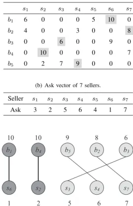
TABLE 2: An illustrative example.

(a) Bid matrix of 5 buyers.

s1 s2 s3 s4 s5 s6 s7

b1 6 0 0 0 5 10 0

b2 4 0 0 3 0 0 8

b3 0 0 6 0 0 9 0

b4 0 10 0 0 0 0 7

b5 0 2 7 9 0 0 0

(b) Ask vector of 7 sellers.

Seller s1 s2 s3 s4 s5 s6 s7

Ask 3 2 5 6 4 1 7

b1 b4 b5 b2 b3

s6 s2 s3 s4 s7

10 10 9 8 6

1 2 5 6 7

Fig. 2: Assignment result with truthful bids and asks: A bipartite graph of matched winning candidates.

adapt to others’ behaviors.

Though truthfulness presents all the aforementioned merits, unfortunately, there is no double auction mechanism that is truthful, efficient2_{, individually rational, and at the same} time balances the budget [4]. In this paper, we design two feasible auction mechanisms that are computationally efficient, individually rational, and budget-balanced. The first mecha-nism TIM further satisfies truthfulness in addition to these three properties. Extending TIM by involving randomness, the second mechanism EDA can achieve a higher system efficiency than that of TIM but truthfulness is guaranteed in a weak sense, i.e., strongly truthful for sellers but truthful in expectation for buyers as demonstrated in the experiment results. Nonetheless, the difficulties in computing an effective lie, combined with the backfire risk of untruthful bid will convince the buyers not to bother to lie.

3.4 Design Rationale

As mentioned in Section 2, there is still room to improve the system efficiency of many existing truthful auction mecha-nisms. To illustrate this, we take the TASC double auction in [10] as an example, and consider a bid matrix of5buyers with true valuations in Table 2(a) and the ask vector of 7 sellers with true costs in Table 2(b).

2. This paper addresses both system efficiency and computational efficiency. To avoid confusion, we use the terms efficient and efficiency to indicate specifically the system efficiency, while we use the terms computationally efficientandcomputational efficiencyto distinguish from system efficiency.

Suppose that the auctioneer uses maximum matching in the assignment stage to maximize the number of matchings. According to the assignment algorithm of TASC, the win-ning buyer candidates, the winwin-ning seller candidates and the mapping between them are shown in Fig. 2. Then, following the TASC strategy for winner-determination & pricing, we have the set of winning buyers Bw = {b1, b4}, the set of

winning sellers Sw={s6, s2}, the clearing pricePwb ={8},

and the clearing paymentPs

w={6}. As seen, the number of

successful trades is only 2.

On the other hand, if the true valuations of buyers and true costs of sellers are known a priori, an optimal strategy can be applied to maximize the number of successful trades. The auctioneer can assign a seller sj to a buyer bi as long as

V_ij ≥ Cj. Then, the auctioneer can select a value between

Cj andVij as the price charged to buyerbi and the payment

rewarded to sellersj, i.e.,Vij ≥Pijb =Pijs ≥Cj. In the given

example, it can be easily shown that this optimal strategy can maximize the number of successful trades to 5. Thus, TASC only achieves 40% of the system efficiency of the optimal strategy. Inspired by this observation, we propose two feasible auction mechanisms. TIM in Section 4 gives a truthful version, while EDA in Section 5 can achieve a higher system efficiency.

4

T

RUTHFUL

I

NCENTIVE

M

ECHANISM

(TIM)

In this section, we present a truthful auction mechanism TIM for resource sharing of cloudlets, which improves the system efficiency over TASC. We first introduce the algorithms of TIM and then give an illustrative example. The properties of TIM are also analyzed in terms of computational efficiency, individual rationality, budget balance and truthfulness. 4.1 Details of TIM

TIM in Algorithm 1 contains two sub-procedures specified in Algorithm 2 and Algorithm 3, which correspond to two stages, Candidate-Determination & Pricing and Candidate-Elimination, respectively.

Algorithm 1 TIM(B,S,D_,A_).

Input: B,S,D_,A Output: Bw,Sw, σ,Pwb,Pws

1: (Bc,Sc,σ,ˆ Pcb,Pcs)←TIM-CD&P(B,S,D,A);

2: (Bw,Sw, σ,Pwb,Pws)←TIM-CE(Bc,Sc,σ,ˆ Pcb,Pcs,D);

3: return(Bw,Sw, σ,Pwb,Pws);

In the candidate-determination & pricing stage, the candi-date determination and pricing operations are coupled together. First, the auctioneer determines the buyer candidate for each seller sj with ask Aj. Then, the price charged to the buyer

candidate and the payment paid to the seller will be determined accordingly. LetA_{−j denote the ask vector excluding the ask}

ofsj, andAo−j be the median ofA−j. The median of a vector

is the value of the middle element in a non-decreasing order of the elements. If there is an even number of values, the mean of the two middle values is defined as the median. According to Algorithm 2, there are two cases in this stage to determine the winning buyer candidate for seller sj.

Algorithm 2 TIM-CD&P(B,S,D_,A_).

Input: B,S,D,A Output: Bc,Sc,σ,ˆ Pcb,Pcs

1: Bc← ∅,Sc← ∅,Pcb← ∅,Pcs← ∅;

2: forsj∈ S do

3: Find the median askAo

−j of the ask vectorA−j;

4: Bj₌

{bi:Dij≥Aj,∀bi∈ B};

5: if|Bj

|= 1then

6: ifD_ij≥Ao

−j andAj≤Ao−jthen

7: σˆ(j) =i,Bc← Bc∪ {bi},Sc← Sc∪ {sj};

8: Pijb =Pjs=Ao−j;

9: Pcb← Pcb∪ {Pijb},Pcs← Pcs∪ {Pjs};

10: end if

11: else if|Bj_|>1then

12: SortBj_toBj _{such thatD}j i(1)≥D

j

i(2) ≥ · · ·;

13: ifD_ij

(1) ≥A

o

−jthen

14: ifthe firstt(t≥2)bids ofBjare the samethen

15: Randomly select bifrom firsttbuyers ofBj;

16: else

17: Select firstbiofBj with the highest bid;

18: end if

19: σˆ(j) =i,Bc← Bc∪ {bi},Sc← Sc∪ {sj};

20: Pijb =Pjs= max{Ao−j, D j i(2)}; 21: Pcb← Pcb∪ {Pijb},Pcs← Pcs∪ {Pjs};

22: end if

23: end if

24: end for

25: return(Bc,Sc,σ,ˆ Pcb,Pcs);

• Only one buyerbiwith a bid not less thanAj: IfDji ≥Ao−j

andAj ≤Ao−j,bi is added into the buyer candidate setBc

with priceAo

−j, andsjis added into the seller candidate set

Sc with paymentAo−j; otherwise, bi cannot winsj.

• Two or more buyers with bids not less than Aj: If the

highest bid is less than Ao

−j, no buyer wins the service of

sj; otherwise, the buyer with the highest bid (or a randomly

selected buyer when there is a tie) is added into the buyer candidate setBc, andsjis added into the seller candidate set

Sc. The price to the selected buyer and the payment to the

corresponding seller is the same as the maximum of Ao

−j

and the second highest bid.

In the candidate-elimination stage, since a buyer candidate inBc may win two or more sellers in the seller candidate set

Sc, Algorithm 3 is run to choose only one best seller for such

a buyer. Specifically, the auctioneer selects the seller so that the corresponding buyer achieves the highest utility. Likewise, when there is a tie in terms of the achievable utilities, one seller is randomly selected. At the end of the candidate elimination stage, every buyerbσ(j)∈ Bwhas a one-to-one mapping with

only one winning sellersj ∈ Sw.

4.2 A Walk-Through Example

To illustrate the procedure of TIM, we use an example with the bid matrix in Table 2(a) and the ask vector in Table 2(b). 1) Candidate-Determination & Pricing:

• B_c =∅,S_c=∅,P_cb=∅,P_cs=∅;

• s1: We have the ask vectorA−1={2,5,6,4,1,7}, and the

median ask Ao

−1 = 4.5. As D11 > A1 and D21 > A1, we

have B1_={b

1, b2}. Since |B1|>1andD11> Ao−1> D12,

Algorithm 3 TIM-CE(Bc,Sc,σ,ˆ Pcb,Pcs,D).

Input: Bc,Sc,σ,ˆ Pcb,Pcs,D Output: Bw,Sw, σ,Pwb,Pws

1: Bw← Bc,Sw← Sc,Pwb← Pcb,Pws ← Pcs,σ←ˆσ;

2: forany two sellerssα, sβ∈ Sw, α6=βdo

3: ifσ(α) =σ(β)then

4: Uσb(j)j=D j σ(j)−P

b

σ(j)j, j={α, β};

5: ifUb

σ(α)α=Uσb(β)β then

6: j′ ←randomly selected from{α, β};

7: else

8: j′_{←arg min}

j∈{α,β} {Uσb(j)j};

9: end if

10: Sw← Sw\ {sj′};

11: Pb

w← Pwb\ {Pσb(j′)j′},Pws ← Pws \ {Pjs′}, σ(j′) =∅;

12: end if

13: end for

14: return(Bw,Sw, σ,Pwb,Pws);

Pb

11 = P1s = Ao−1. Therefore, we have σˆ(1) = 1,Bc ←

Bc ∪ {b1},Sc ← Sc ∪ {s1}, P11b = P1s = Ao−1, Pcb ←

Pb

c ∪ {P11b},Pcs ← Pcs∪ {P1s}. As a similar procedure is

applied to examine other sellers inS, we skip the details in the following to avoid repetition;

• s2:B2={b4, b5},Ao−2= 4.5. Since D25< Ao−2< D24, we

have σˆ(2) = 4,Bc ← Bc∪ {b4},Sc ← Sc ∪ {s2}, P42b =

P2s=Ao−2, Pcb← Pcb∪ {P42b},Pcs← Pcs∪ {P2s};

• s3:B3={b3, b5},Ao−3= 3.5. Since Ao−3< D33< D35, we

have σˆ(3) = 5,Bc ← Bc∪ {b5},Sc ← Sc ∪ {s3}, P53b =

Ps

3=D33,Pcb← Pcb∪ {P53b},Pcs← Pcs∪ {P3s};

• s4: B4 = {b5}, A−o4 = 3.5. Since Ao−4 < A4, no buyer

wins the service froms4;

• s₅:B5_={b

1},Ao−5= 4. SinceA5=Ao−5< D51, we have

ˆ

σ(5) = 1,Bc ← Bc∪ {b1},Sc ← Sc∪ {s5}, P15b =P5s =

Ao

−5,Pcb← Pcb∪ {P15b},Pcs← Pcs∪ {P5s};

• s6:B6={b1, b3},Ao−6= 4.5. Since Ao−6< D63< D61, we

have σˆ(6) = 1,Bc ← Bc∪ {b1},Sc ← Sc ∪ {s6}, P16b =

Ps

6=D63,Pcb← Pcb∪ {P16b},Pcs← Pcs∪ {P6s};

• s7:B7={b2, b4},Ao−7= 3.5. Since Ao−7< D74< D72, we

have σˆ(7) = 2,Bc ← Bc∪ {b2},Sc ← Sc ∪ {s7}, P27b =

P7s=D74,Pcb← Pcb∪ {P27b},Pcs← Pcs∪ {P7s};

• In summary, Algorithm 2 gives the following output:

– Bc={b1, b2, b4, b5};

– Sc={s1, s2, s3, s5, s6, s7};

– Pb

c ={P11b = 4.5, P42b = 4.5, P53b = 6, P15b = 4, P16b =

9, Pb 27= 7};

– Ps

c = {P1s = 4.5, P2s = 4.5, P3s = 6, P5s = 4, P6s =

9, Ps 7= 7};

– σˆ ={σˆ(1) = 1,ˆσ(2) = 4,σˆ(3) = 5,ˆσ(5) = 1,σˆ(6) = 1,σˆ(7) = 2}.

2) Candidate-Elimination:

The output of Algorithm 2 includes σˆ(1) = ˆσ(5) = ˆ

σ(6) = 1, which means buyer candidateb1 wins three seller

candidates, i.e.,s1,s5ands6. Algorithm 3 is run subsequently

to retain one best seller for buyerb1. The utilities ofb1with

re-spect to the three seller candidates are computed and given by: Ub

11=D11−P11b = 6−4.5 = 1.5,U15b =D15−P15b = 5−4 = 1,

Ub

16=D61−P16b = 10−9 = 1. Clearly,s1results in the highest

utility forb1. Thus,s5ands6are eliminated from the winning

seller set. In conclusion, Algorithm 3 produces the following

auction outcome: • B_w={b1, b2, b4, b5};

• S_w={s1, s2, s3, s5, s6, s7} \ {s5, s6}={s1, s2, s3, s7};

• P_wb = {P₁₁b, P₄₂b, P₅₃b, P₁₅b, P₁₆b, P₂₇b} \ {P₁₅b, P₁₆b} = {Pb

11, P42b, P53b, P27b} = {P1b = 4.5, P4b = 4.5, P3b =

6, Pb 2 = 7};

• P_ws = {P₁s, P₂s, P₃s, P₅s, P₆s, P₇s} \ {P₅s, P₆s} = {P₁s =

4.5, Ps

2 = 4.5, P3s= 6, P7s= 7};

• σ={σ(1) = 1, σ(2) = 4, σ(3) = 5, σ(7) = 2}. 4.3 Proof of Desirable Properties

In the following, we prove that TIM holds the properties of computational efficiency, individual rationality, budget balance and truthfulness.

Theorem 1. TIM is computationally efficient.

Proof. To implement Algorithm 2 for the candidate-determination & pricing stage, we can first sort the sellers in S with a time complexity of O(mlogm). Then, within the for-loop in Algorithm 2, the median of the ask vector

A_{−j can be obtained in O(1) time. In Line 4, finding B}j

has a time complexity of O(n), while sorting Bj _{to B}j _in

Line 12 has a time complexity of O(nlogn). Since there are at most n buyers in Bj_{, the buyer candidate for each seller}

can be determined inO(n)time. Thus, each round of the for-loop takes O(nlogn)time. In total, Algorithm 2 has a time complexity ofO(mlogm+mnlogn).

In the candidate-elimination stage, the input to Algorithm 3 apparently satisfies |Sc| ≤ |S| ≤ m. Hence, the for-loop in

Algorithm 3 spendsO(|Sc|(|Sc|−1)

2 ) =O(m

2_{)time. Therefore,}

the overall time complexity of TIM is polynomial in the order ofO(m2_+mnlogn).

Theorem 2. TIM is individually rational.

Proof. In Algorithm 2, there are two cases for buyerbi to be

selected as a buyer candidate (bi ∈ Bc) and for sellersj to

become a seller candidate(sj ∈ Sc).

• |Bj| = 1: This case results in a buyer candidatebi and a

seller candidate sj only if Dji ≥Ao−j ≥Aj. The clearing

price charged to buyer bi and the payment to sellersj are

bothAo

−j.

• |Bj| > 1: In this case, buyer bi must have a bid Dij not

less thanAo

−j andD j

i is the highest bid for sellersj, which

implies that Ao

−j ≤D j

i andD

j

i(2) ≤D

j

i. The clearing price

and payment are the maximum ofDj_i(2) andAo

−j. Besides,

every qualified buyer in Bj _{must bid not less thanA} j.

As seen, each buyer candidate determined in Algorithm 2 is never charged a price greater than its bid, while each seller candidate is rewarded a payment not less than its ask, which ensures individual rationality for both buyers and sellers.

It is possible for Algorithm 2 to assign multiple sellers to one buyer candidate bi ∈ Bc. Algorithm 3 eliminates

redundant sellers and keeps only one best seller providing buyer bi the highest utility. It is evident that this procedure

does not change the charging pricePb

ij to the winning buyers.

still satisfy individual rationality. On the other hand, a seller candidatesj is either a winning seller with the same payment

Ps

j determined in Algorithm 2, or eliminated with zero

pay-ment at zero cost. Therefore, individual rationality still holds for the winning sellers in Sw resulted from Algorithm 3.

In conclusion, TIM is individually rational.

Theorem 3. TIM is budget-balanced.

Proof. After the candidate-elimination stage, every winning buyer bi ∈ Bw has only one winning seller sj ∈ Sw.

Considering this one-to-one mapping between Bw and Sw,

we have |Bw|=|Sw|. The clearing price and payment satisfy

Pb

i =Pjsfor each winning buyerbiand its assigned matching

seller sj, i.e.,σ(j) =i. Therefore, it can be easily shown that

X

bi∈Bw

P_ib− X

sj∈Sw

P_js= X

sj∈Sw

P_σ(j)b −P_js= 0

which completes the proof.

Theorem 4. TIM is truthful.

Theorem 4 can be proved by the following Lemma 1 and Lemma 2, which show that TIM is truthful for sellers and buyers, respectively.

Lemma 1. TIM is truthful for sellers.

Proof. To compare the auction outcomes with truthful or any arbitrary asks, we add tilde in the notations for the general (untruthful) cases. To prove Lemma 1, we divide the seller set S into three subsets:Sw,Sc\ Sw andS \ Sc.

1) For seller sj ∈ Sw: There are two cases when sj asks

untruthfully.

• Sellersj ∈ S/ w: Uejs= 0≤Ujs.

• Sellersj ∈ Sw: There are four subcases.

– |Bj_{|= 1and|Be}j_{|= 1: Pe}s

j =Pjs=Ao−j.

– |Bj_{|= 1and|Be}j_{|>1: Ae}

j< Cj,Pejs=Pjs=Ao−j.

– |Bj_|>1and|Bej_{|= 1: Ae}

j> Cj,Pejs=Pjs=Ao−j.

– |Bj_|>1and|Bej_{|>1: Pe}s

j =Pjs=Ao−j orD j i(2).

Thus, we haveUejs=Pejs−Cj=Pjs−Cj =Ujs.

2) For sellersj∈ Sc\ Sw:sjcannot be inSwno matter what

valueAej is. Thus, we have Uejs= 0 =Ujs.

3) For seller sj ∈ S \ Sc: There are two cases when sj asks

untruthfully.

• Sellersj ∈ S/ w: Uejs= 0 =Ujs.

• Sellersj∈ Sw: Letbibe the buyer that winssj at price

e Pb

ij =Pejs whensj asks untruthfully. Here, we consider

two subcases to compare the utilities.

– |Bj_{|= 0: We know thatC}

j is greater than any bid of

the buyers. According to Theorem 2, the buyers satisfy individual rationality so thatD_ij≥Peb

ij. Thus, we have

Cj > Dij≥Peijb=Pejs, andUejs=Pejs−Cj<0 =Ujs.

– |Bj_{| = 1, and A}o

−j < Aj = Cj ≤ Dji: The reason

thatsj ∈ Sw when sj asks untruthfully is thatAej ≤

Ao

−j and/or |Bej| ≥2. Additionally, buyerbi needs to

pay Peb

ij = Ao−j or De j

i(2), where De j

i(2) is the second

highest bid of the buyers in Bej_{. However, we know}

thatAo

−j< Aj =Cj andDej_i(2) < Aj =Cj. Thus, we

havePes

j =Peijb < Cj, andUejs=Pejs−Cj <0 =Ujs.

As seen, telling truth provides the maximum utility for each seller in TIM. Therefore, truthful asking is a weakly dominant strategy for sellers in TIM, which proves Lemma 1.

Lemma 2. TIM is truthful for buyers.

Proof. Similarly, we add tilde in the notations for the out-comes with general (untruthful) bids. Here, we divide the buyer set Binto two subsets: Bw andB \ Bw.

1) For buyer bi ∈ Bw: Assuming buyer bi wins seller sj

with truthful bidding, we consider three cases whenbibids

untruthfully.

• Buyerbi loses:Ueib= 0≤Uib.

• Buyerbi still winssj: According to Algorithm 2, since

the clearing price is independent of the bid of buyerbi,

we have Peb

ij =Pijb, and thusUeib=Ueijb =V j

i −Peijb =

Ub i.

• Buyerbi wins sellersj′: There are two subcases.

– Seller sj′ ∈ S_c when buyerb_i bids truthfully:

∗ σˆ(j′) = i with truthful bid D_{i: According to}

Algorithm 2, we havePeb

ij′ =P_ijb′. The reason that

buyer bi wins seller sj when it bids truthfully is

Ub

ij≥Uijb′, whereU_ijb′ =V

j′

i −Pijb′. As a result, we

haveUeb

i =Ueijb′ =V

j′

i −Peijb′ =U_ijb′ ≤Uijb =Uib.

∗ σˆ(j′_{) 6= i with truthful bid D}

i: According to

Algorithm 2, there exists a buyer candidatei′ _with Dj_i′′ ≥D

j′

i =V

j′

i . When bidding untruthfully,

buy-er bi wins seller sj′ with pricePe_ijb′ ≥D

j′

i′ ≥V

j′

i .

Thus,Ueb

i =Ueijb′ =V

j′

i −Peijb′ ≤0≤U_ib.

– Seller sj′ ∈ S/ _c when buyerb_i bids truthfully:

∗ Truthful bid Dj_i′ is less than ask Aj′: When buyer

bi bids untruthfully, it paysPeijb′ to win sellersj′.

According to Theorem 2, the sellers satisfy individ-ual rationality so that Peb

ij′ ≥Aj′ > Dj ′

i =V

j′

i . As

a result,Ueb

i =Ueijb′ =V

j′

i −Peijb′ <0≤U_ib.

∗ Truthful bid D_ij′ is not less than ask Aj′, and

Ao

−j′ > D

j′

i =V

j′

i : When buyerbibids

untruthful-ly, it paysPeb

ij′ =Ao−j′ to win sellersj′. As a result,

we still have Ueb

i =Ueijb′ =V

j′

i −Peijb′ <0≤Uib.

2) For buyerbi∈ B \ Bw: Obviously,Uib= 0. There are two

cases whenbi bids untruthfully.

• Buyerbi still loses:Ueib= 0 =Uib.

• Buyerbi wins sellersj: There are three subcases.

– Truthful bid D_ij is less than ask Aj: When buyerbi

with untruthful bid wins seller sj at price Peij, the

seller should satisfy individual rationality according to Theorem 2, so that Peb

ij ≥Aj > Dji = V j i. As a

result, we haveUeb

i =Ueijb =V j

i −Peijb <0 =Uib.

– Truthful bid Dj_i is not less than ask Aj, and Ao−j >

Dj_i = V_ij: When buyer bi bids untruthfully, it wins

know thatPeb

ij ≥ Ao−j > V j

i , and thus Ue b

i =Ueijb =

V_ij−Peb

ij <0 =Uib.

– Truthful bid Dj_i is not less than ask Aj, Dji > Ao−j,

and there exists buyerbi′ with bid Dj_i′ ≥D

j

i =V

j i :

When buyerbibids untruthfully, it paysPeijb≥D j i′ to

win sellersj. Thus, we haveUeib=Ueijb =V j

i −Peijb≤

0 =Ub i.

Therefore, telling truth maximizes the utility of each buyer in TIM and Lemma 2 is proved.

5

E

FFICIENT

D

ESIGN OF

A

UCTION

(EDA)

In Section 4, we introduce the truthful incentive mechanism TIM, which is proved to hold the desirable properties of computational efficiency, individual rationality, budget balance and truthfulness. Unfortunately, a double auction mechanism cannot further achieve system efficiency (e.g., maximizing social welfare) at the same time [4]. In this section, we present another more efficient design of auction EDA, which slightly relaxes the truthfulness constraint and ensures truthfulness in a weak sense. We follow the same sequence as Section 4, giving the detailed algorithm of EDA, then an illustrative example, and the analysis of its properties at last.

5.1 Details of EDA

As illustrated in Section 4.2, the buyer candidateb1wins three

seller candidates(s1,s5ands6), and only the seller candidate

s1becomes a winning seller inSw. The other seller candidates

s5 and s6 are not successfully matched to potential buyers,

which degrades the system efficiency and thus jeopardizes the utilization of MCC resources. EDA improves the system efficiency by involving randomness and more uncertainty in the auction mechanism.

The details of EDA are given in Algorithm 4. According to EDA, the auctioneer first constructs a randomly ordered list

S _{of the seller set S, then determines the winning buyer for}

each seller sj∈ S following the order of S. Recall thatA−j

denotes the ask vector without the ask ofsj, andAo−j is the

median ask ofA_{−j. LetB}j _{be the sublist of buyers inB \ Bw}

with bids not less than the ask of sellersj. Then, Algorithm 4

handles two different cases as follows.

• |Bj|= 1: Assume that bi is the buyer in Bj with bidDji.

Among all the bids of buyers for sellersj, denoted byDj,

let Dj_i∗ be the highest bid in Dj that is less thanD

j i, and

Pbs _{be the maximum ofA}o

−j andD j i∗. IfD

j

i ≥Pbs≥Aj,

thenbi is added intoBwand assigned a clearing pricePbs,

whilesj is added intoSwwithPbsas the clearing payment.

IfD_ij< Pbs _orA

j > Pbs,bi cannot win the service ofsj.

• |Bj| > 1: If the highest bid of the buyers in Bj _{is less}

thanAo

−j, no buyer obtains the service ofsj; otherwise, the

buyerbi∈ Bj with the highest bid (or a randomly selected

buyer when there is a tie) winssj. Then, buyerbi and seller

sj are added intoBwandSw, respectively. LetDji(2) be the

second highest bid of the buyers in Bj_{, and D}j

i∗ be the

highest bid inDj _{that is less thanD}j

i. Note thatDj is the

bid vector of all buyers for sellersj, whileBjonly includes

Algorithm 4 EDA(B,S,D_,A_).

Input: B,S,D,A Output: Bw,Sw, σ,Pwb,Pws

1: Bw← ∅,Sw← ∅,Pwb ← ∅,Pws ← ∅;

2: Randomly orderS to obtainS={sr₍₁₎, sr₍₂₎, . . . , sr_(m)};

3: forsj∈ S in the order ofSdo

4: Find the median askAo

−j of the ask vectorA−j;

5: Bj₌

{bi:Dij≥Aj,∀bi∈ B \ Bw};

6: if|Bj

|= 1then

7: Find highest bidD_ij∗ ∈D

j

that is not greater thanDji;

8: Pbs= max{Ao−j, Dji∗};

9: ifD_ij≥Pbs andAj≤Pbs then

10: σ(j) =i,Bw← Bw∪ {bi},Sw← Sw∪ {sj};

11: Pijb =Pjs=Pbs;

12: Pwb ← Pwb∪ {Pijb},Pws ← Pws ∪ {Pjs};

13: end if

14: else if|Bj

|>1then

15: SortBj

to get Bjsuch thatDj_i

(1)≥D

j

i(2) ≥ · · ·; 16: Find highest bidDj_i∗ ∈D

j_{that is not greater thanD}j i(1);

17: ifD_ij

(1) ≥A

o

−jthen

18: ifthe firstt(t≥2)bids ofBj_{are the samethen}

19: Randomly select bifrom firsttbuyers ofBj;

20: else

21: Select first buyer biofBj with the highest bid;

22: end if

23: σ(j) =i,Bw← Bw∪ {bi},Sw← Sw∪ {sj};

24: Pijb =Pjs= max{Ao−j, D j i∗};

25: Pb

w← Pwb∪ {Pijb},Pws ← Pws ∪ {Pjs};

26: end if

27: end if

28: end for

29: return(Bw,Sw, σ,Pwb,Pws);

the remaining buyers that have bids not less than Aj and

are still competing. The clearing price charged tobiand the

payment rewarded tosj are both the maximum ofAo−j and

Dj_i∗.

As seen in Line 5, the winning buyers inBware eliminated in

the buyer sublistBj_{. Thus, a winning buyerb}

i ∈ Bw will not

compete with other buyers for the remaining sellers. Hence, it is not necessary to include candidate elimination as in TIM and the system efficiency is improved as a result.

5.2 A Walk-Through Example

For easy comparison, the following illustrative example for EDA is also based on the bid matrix in Table 2(a) and the ask vector in Table 2(b). Applying Algorithm 4, we have • Bw=∅,Sw=∅,Pwb=∅,Pws =∅;

• Suppose that the seller set S is randomly ordered to S = {s3, s5, s7, s1, s4, s6, s2};

• s3: Similar to the walk-through example for TIM, we only

provide the details for this case to save space. First, we have the ask vectorA_{−3={3,2,6,4,1,7}, and its median}

Ao

−3= 3.5. Sinceb3∈ B \ BwwithD33> A3, andb5∈ B \

Bw withD35> A3, we obtainB3={b3, b5}. As|B3|>1,

D3

5∗ = 6andD53> D35∗ =D33> Ao−3,b5is selected as the

winning buyer fors3 withP53b =P3s=D35∗. Therefore, we

have σ(3) = 5,Bw← Bw∪ {b5},Sw ← Sw∪ {s3}, P53b =

Ps

3 =D35∗,Pwb ← Pwb∪ {P53b},Pws ← Pws ∪ {P3s};

• s5: B5 = {b1}. Since D51∗ = 0, Ao−5 = 4, Pbs = Ao−5

{b1},Sw ← Sw∪ {s5}, P15b = P5s = Pbs,Pwb ← Pwb ∪

{Pb

15},Pws ← Pws ∪ {P5s};

• s7: B7 = {b2, b4}. Since Ao−7 = 3.5 < D47 = D27∗ <

D7

2, we have σ(7) = 2,Bw ← Bw∪ {b2},Sw ← Sw∪

{s7}, P27b =P7s =D27∗, P_wb ← P_wb∪ {P27b},Pws ← Pws ∪

{Ps 7};

• s₁:B1_{=∅. No buyer wins the service ofs} 1;

• s₄:B4_{=∅. No buyer wins the service ofs} 4;

• s6: B6 = {b3}. Since D63∗ = 0, Ao−6 = 4.5, Pbs = Ao−6

and A6 < Pbs < D63, we have σ(6) = 3,Bw ← Bw∪

{b3},Sw ← Sw∪ {s6}, P36b = P6s = Pbs, Pwb ← Pwb ∪

{Pb

36},Pws ← Pws ∪ {P6s};

• s2: B2 = {b4}, since D42∗ = 2, Ao₋₂ = 4.5, Pbs = Ao₋₂

and A2 < Pbs < D24, we have σ(2) = 4,Bw ← Bw∪

{b4},Sw ← Sw∪ {s2}, P42b = P2s = Pbs, Pwb ← Pwb ∪

{Pb

42},Pws ← Pws ∪ {P2s};

• In summary, Algorithm 4 gives the auction outcome:

– Bw={b1, b2, b3, b4, b5};

– Sw={s2, s3, s5, s6, s7};

– Pb

w = {P42b = 4.5, P53b = 6, P15b = 4, P36b = 4.5, P27b =

7};

– Ps

w={P2s= 4.5, P3s= 6, P5s= 4, P6s= 4.5, P7s= 7};

– σ ={σ(2) = 4, σ(3) = 5, σ(5) = 1, σ(6) = 3, σ(7) = 2};

As seen, the system efficiency of EDA is improved to 5

successful matchings as opposed to 4 in TIM. It is worth noting that the performance of Algorithm 4 may depend on the ordered list S_{. The auctioneer can generate multiple random}

lists to obtain an outcome of the highest system efficiency. 5.3 Proof of Desirable Properties

Similar to TIM, EDA also satisfies computational efficiency, individual rationality and budget balance. Nonetheless, as mentioned earlier, EDA achieves a higher system efficiency but at the cost of weaker truthfulness.

Theorem 5. EDA is computationally efficient.

Proof. According to the ask vector of sellers, we can first sort the sellers in S in a non-decreasing order of their asks, which has a time complexity of O(mlogm). In each round of the for-loop in Algorithm 4, we can spend O(1) time to determine the median of the ask vectorA_{−j, andO(n)time to}

obtainBj_{. In addition, findingD}j

i∗ runs inO(n)time. When

|Bj_{| > 1, sorting B}j _{to B}j _{further takes O(nlogn) time,}

while the winning buyer can be selected in O(n) time since there are at most n buyers in Bj_{. Thus, each round of the}

for-loop spendsO(nlogn)time. The overall time complexity of Algorithm 4 is thenO(mlogm+mnlogn).

Theorem 6. EDA is individually rational.

Proof. Consider a pair of matched buyer and seller, bi and

sj, in the winning sets Bw and Sw. There are two cases for

Algorithm 4 to assign this matching.

• |Bj|= 1: In this case, bi wins the service ofsj only when

Dj_i ≥Pbs_≥A

j. The clearing price and payment are both

Pbs_{, which is not greater than the bid of b}

i and not less

than the ask ofsj.

• |Bj|>1: In this case,bi must have a bidDj_i not less than

Ao

−j andD j

i is the highest bid inBj. Thus, we haveAo−j ≤

Dj_i and Dj_i∗ ≤ D

j

i. Since the clearing price and payment

are the maximum ofAo

−jandD j

i∗, the preceding conditions

imply that the price charged to buyerbiis not greater than its

bidDj_i. On the other hand, we haveD_ij∗ ≥Aj. This can be

easily inferred from the definition thatDj_i∗ is the highest bid

not greater thanD_ijinDj_{, and the fact thatD}j

i is the highest

bid in Bj_{. Since|B}j_{|>1and every buyer inB}j _{has a bid}

not less thanAj, we haveDji =D j

i(1) ≥D

j

i∗ ≥D

j

i(2)≥Aj.

Here, D_i(1)j andD_i(2)j are the first and second highest bids inBj_{, respectively. Thus, the clearing payment tos}

j should

be not less than Aj.

As seen in both cases, each winning buyer determined in Algorithm 4 never pays more than its bid, while each winning seller is paid not less than its ask, which guarantees individual rationality for buyers and sellers.

Theorem 7. EDA is budget-balanced.

Proof. In the auction outcome, EDA keeps one-to-one map-ping between Bw and Sw as TIM, while the clearing price

charged to a winning buyer is equal to the clearing payment to the matched winning seller. Thus, we can easily show that EDA is budget-balanced by applying the proof of budget balance of TIM.

5.3.1 Truthfulness of EDA for Sellers

Theorem 8. EDA is truthful for sellers.

Proof. Similar to the proof of truthfulness of TIM for sellers, we consider two subsets of the seller setS:Sw andS \ Sw.

1) For seller sj ∈ Sw: There are two cases when seller sj

asks untruthfully.

• Seller sj∈ S/ w:Uejs= 0≤Ujs.

• Seller sj ∈ Sw: There are four subcases with respect

to |Bj_{| = 1 or |B}j_{| > 1, and |Be}j_{| = 1 or |Be}j_{| > 1.}

In all these subcases, we can infer from Algorithm 4 that Pes

j = Pjs = max{Ao−j, D j

i∗}. Therefore, we have

e Us

j =Pejs−Cj=Pjs−Cj =Ujs.

2) For sellersj ∈ S \ Sw: There are two cases when sellersj

asks untruthfully.

• Seller sj∈ S/ w:Uejs= 0 =Ujs.

• Seller s_j ∈ S_w: Letb_i be the buyer that wins seller s_j at price Peb

ij =Pejs. There are two subcases to examine

the utilities of different asks.

– |Bj_{|= 0: That isD}j

i < Aj=Cj. According to

Theo-rem 6, the buyers satisfy individual rationality, so that Dj_i ≥Peb

ij. As a result, we haveCj > Dji ≥Peijb =Pejs,

andUes

j =Pejs−Cj<0 =Ujs.

– |Bj_{| = 1, and max{A}o

−j, D j

i∗} < Aj = Cj ≤ D

j i:

When seller sj asks untruthfully, sj ∈ Sw only if

e

Aj ≤ max{Ao−j, D j

i∗} and/or |Bej| ≥ 2. The price

charged to buyer bi is then Peijb = max{Ao−j, D j i∗}.

Since max{Ao

−j, D j

i∗} < Aj = Cj, we have Pejs =

e Pb

As seen, telling truth is a weakly dominant strategy for sellers in EDA, which proves Theorem 8.

5.3.2 Truthfulness of EDA for Buyers

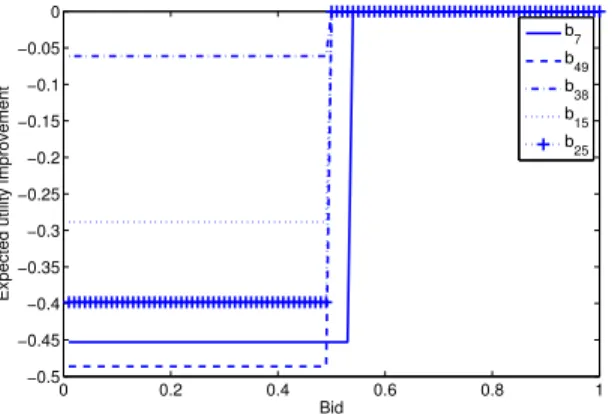
Theorem 8 shows that EDA is strongly truthful for sellers. However, EDA cannot maintain strong truthfulness for buy-ers. Fortunately, the following analysis also shows that the uncertainty and randomness in EDA introduce high risks and difficulties for buyers to bid untruthfully to improve their utilities. A truthful bid can always lead to a non-negative utility, whereas bidding untruthfully may result in a non-positive utility. Therefore, EDA can ensure truthfulness for buyers in a weak sense. As further demonstrated in the experiment results, EDA achieves truthfulness in expectation. When bidding truthfully, a buyer in B can fall into either subset Bw or subsetB \ Bw. First, we prove that telling truth

is a weakly dominate strategy for buyer bi ∈ B \ Bw as it

maximizes the buyer’s utility. There are two cases when bi

bids untruthfully.

• Buyerbi still loses:Ueib= 0 =Uib.

• Buyerbi wins seller sj: There are three subcases.

– Truthful bid Dj_i is less than ask Aj: According to

Theorem 6, the sellers satisfy individual rationality, so we have Peijb ≥ Aj > Dij = V

j

i . As a result, we have

e Ub

i =Ueijb =V j

i −Peijb <0 =Uib.

– Truthful bidDj_i is not less than askAj, andAo−j> D j

i =

V_ij: When buyer bi bids untruthfully, it wins seller sj at

pricePeb

ij. According to Algorithm 4, we know thatPeijb≥

Ao

−j> V j

i , and thusUeib=Ueijb =V j

i −Peijb <0 =Uib.

– Truthful bidDj_i is not less than askAj,Dji > Ao−j, and

there exists a buyerbi′ ∈ B\Bwwith bidDj_i′ ≥D

j

i =V

j i :

When buyer bi bids untruthfully, it pays Peijb ≥ D j i′ to

win seller sj. As a result, we still have Ueib = Ueijb =

V_ij−Peb

ij ≤0 =Uib.

Second, we show two situations that buyer bi ∈ Bw can

improve its utility by bidding untruthfully.

1) When buyer bi wins seller sj with truthful bid Dji =V j i

and price Pijb = D j

i∗, buyer bi can submit an untruthful

bid Dej_i which is slightly smaller than D_ij∗, so that buyer

bi still wins sellersj but leads to a new pricePeijb =Ao−j.

2) When bidding truthfully, buyer bi has the highest bids for

sellers sα andsβ among all buyers inB \ Bw, and seller

sα appears before sellersβ inS. In this situation, buyerbi

can bid untruthfully withDeα

i = 0to lose seller sα, so that

it wins seller sβ for a higher utility.

Although the buyers in Bw can improve utility in

prin-ciple by bidding untruthfully, there are some difficulties in computing an effective lie. Without the knowledge of the others’ bids, a buyer has no way to determine the auction outcome, such as whether the buyer could win with truthful bid, the matched seller if the buyer wins, and the clearing price. Thus, it is very hard for a buyer to improve its utility by bidding untruthfully. As shown in the preceding discussion, when buyerbi∈ B \ Bwwith truthful bid, bidding untruthfully

cannot result in a positive utility to exceed the zero utility with truthful bid. When buyer bi ∈ Bw with truthful bid, we take

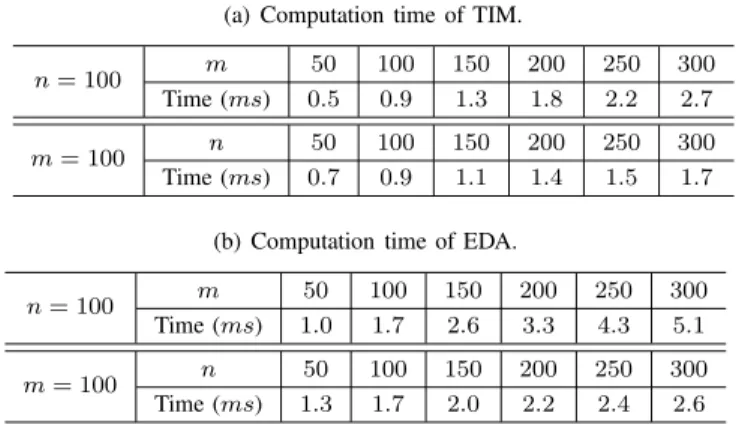
TABLE 3: Computational efficiency.

(a) Computation time of TIM.

n= 100 m 50 100 150 200 250 300

Time (ms) 0_.5 0_.9 1_.3 1_.8 2_.2 2_.7

m= 100 n 50 100 150 200 250 300

Time (ms) 0_.7 0_.9 1_.1 1_.4 1_.5 1_.7

(b) Computation time of EDA.

n= 100 m 50 100 150 200 250 300

Time (ms) 1_.0 1_.7 2_.6 3_.3 4_.3 5_.1

m= 100 n 50 100 150 200 250 300

Time (ms) 1_.3 1_.7 2_.0 2_.2 2_.4 2_.6

the second situation above as an example. If buyer bi wants

to lose sellersα to improve its utility, buyerbi must submit a

zero bid, i.e.,Deα

i = 0, since buyer bi does not know the bids

of other buyers. There is also a risk that buyerbimay achieve

zero utilityUeb

i = 0, if it cannot win a seller other thansα.

Furthermore, supposing complete information of the bid matrix D _{and the ask vector} A _{is publicly known, due to}

the randomness introduced in EDA, an untruthful bid may even backfire to a buyer who should win with truthful bid but lose the auction with a lie. Take the first situation above as an example. Even with the knowledge of D_andA_{, buyer}

bi cannot determineBj, since Bj depends on the randomly

ordered list S_{. Thus, if buyer bi wants to improve its utility}

with a bidDej_i < Dj_i∗, it may experienceUeib= 0, sincebi∗ is

still inB \ Bw.

6

N

UMERICAL

R

ESULTS

This section presents the numerical results to evaluate the performance of TIM and EDA. As seen in the proof in Section 4.3 and Section 5.3, TIM and EDA satisfy desirable properties including computational efficiency, individual ratio-nality, budget balance, and truthfulness. The proof does not set any presumption on the bids of buyers or the asks of sellers. Thus, the conclusions are valid for any possible data sets of the bids and asks. Thus, without loss of generality, we randomly generate the bids of buyers and the asks of sellers according to a uniform distribution within(0,1]unless otherwise specified. For the simulations regarding each desirable property, we also vary the number of buyers or sellers, the bids of buyers, or the asks of sellers, which are detailed in each subsection.

6.1 Computational Efficiency

To confirm our analysis on time complexity of TIM in Theo-rem 1 and that of EDA in TheoTheo-rem 5, we give the computation time of TIM and EDA with different settings in Table 3. For each setting, we randomly generate1000instances and average the results. All the tests run on a Windows PC with 3.16 GHz Intelr CoreTM2 Duo processor and 4 GB memory. As seen, both TIM and EDA are subject to polynomial computation time with respect tonandm, which are the number of buyers and sellers, respectively.

0 5 10 15 20 25 30 0

0.2 0.4 0.6 0.8 1 1.2

Winning buyer−seller pairs

Bid Pricing Ask

(a) TIM.

0 5 10 15 20 25 30 35

0 0.2 0.4 0.6 0.8 1 1.2

Winning buyer−seller pairs

Bid Pricing Ask

(b) EDA.

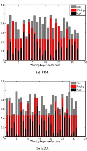
Fig. 3: Individual rationality of TIM and EDA. 6.2 Individual Rationality and Budget Balance To validate Theorem 2 and Theorem 6 regarding individual rationality of TIM and EDA, we show the bids, pricing, and asks in Fig. 3. Since the price charged to each winning buyer Pb

ij is equal to the payment rewarded to each winning seller

Ps

j, the pricing here presents both. As seen, for both TIM

and EDA, each winning buyer is charged a price not higher than its bid, while each winning seller receives a payment not less than its ask from the auctioneer. Therefore, both TIM and EDA are individually rational. The results demonstrate that the cloudlets receive sufficient compensations to be incentivized to share their resources. On the other hand, the mobile users are allocated the demanded resources and pay no more than their valuations of these resources. Thus, the mobile users are also stimulated to request services from the cloudlets.

In addition, sincePb

ij =Pjsfor all the winning pairs in TIM

and EDA, budget balance is also achieved in both mechanisms, which confirms Theorem 3 and Theorem 7 for budget balance of TIM and EDA. Hence, the auctioneer can assist the resource allocation without a deficit.

6.3 Truthfulness of TIM

To verify the truthfulness of TIM, we randomly choose several buyers/sellers to examine how their utilities change when they bid or ask different values. The results are depicted in Fig. 4. Fig. 4(a) shows the case that buyer bi wins seller sj and

gains utility Ub

i = 0.2885 when it bids truthfully withD j

i =

0 0.2 0.4 0.6 0.8 1 0

0.1 0.2 0.3

Bid

Utility

(a) Buyerbi∈ Bw.

0 0.2 0.4 0.6 0.8 1

−0.5 −0.4 −0.3 −0.2 −0.1 0

Bid

Utility

(b) Buyerbi∈ B/ w.

0 0.2 0.4 0.6 0.8 1

−0.05 0 0.05 0.1 0.15 0.2

Ask

Utility

(c) Sellersj∈ Sw.

0 0.2 0.4 0.6 0.8 1

−0.1 −0.05 0 0.05

Ask

Utility

(d) Sellersj∈ S/ w. Fig. 4: Truthfulness of buyers and sellers with TIM.

0 0.2 0.4 0.6 0.8 1 0

0.1 0.2 0.3 0.4

Ask

Utility

(a) Sellersj∈ Sw.

0 0.2 0.4 0.6 0.8 1

−0.2 −0.15 −0.1 −0.05 0 0.05

Ask

Utility

(b) Sellersj∈ S/ w. Fig. 5: Truthfulness of sellers with EDA.

Vij= 0.7875. It can be seen that buyerbi cannot improve its

utility no matter what other bids it takes. Fig. 4(b) shows a different scenario that buyerbi does not win seller sj when

it bids truthfully with Dj_i =V_ij = 0.0437. Thus,bi achieves

zero utility without having the service. Fig. 4(b) shows that the utility cannot be greater than zero even when buyerbibids

untruthfully. Fig. 4(c) shows an example that seller sj wins

when asking truthfully withAj =Cj = 0.3841and achieves

utility Ujs = 0.1528. As seen, the utility with a truthful ask

is the highest among all possible asks. Fig. 4(d) shows that sellersjloses when asking truthfully withAj=Cj= 0.5501

and thus obtains zero utility. For all other asks, the achievable utility is either zero or negative, but cannot be more than zero. In summary, TIM guarantees truthfulness for both buyers and sellers since the utility cannot be improved by bidding or asking untruthfully. In addition, as seen in Fig. 4(a) and Fig. 4(c), the winning mobile user and the cloudlet that are matched successfully gain positive utilities, which means that both benefit from using or providing the demanded resources. 6.4 Truthfulness of EDA

Fig. 5 and Fig. 6 evaluate the truthfulness of EDA for sellers and buyers, respectively.

Fig. 5(a) shows an example with a randomly chosen winning seller sj that asks truthfully with Aj = Cj = 0.0926 and

achieves utility Us

j = 0.4064. As seen, the utility with a