Systems Control With Generalized Probabilistic
Fuzzy-Reinforcement Learning
William M. Hinojosa, Samia Nefti
, Member, IEEE
, and Uzay Kaymak
, Member, IEEE
Abstract—Reinforcement learning (RL) is a valuable learning method when the systems require a selection of control actions whose consequences emerge over long periods for which input– output data are not available. In most combinations of fuzzy sys-tems and RL, the environment is considered to be deterministic. In many problems, however, the consequence of an action may be uncertain or stochastic in nature. In this paper, we propose a novel RL approach to combine the universal-function-approximation ca-pability of fuzzy systems with consideration of probability distri-butions over possible consequences of an action. The proposed generalized probabilistic fuzzy RL (GPFRL) method is a modified version of the actor–critic (AC) learning architecture. The learning is enhanced by the introduction of a probability measure into the learning structure, where an incremental gradient–descent weight– updating algorithm provides convergence. Our results show that the proposed approach is robust under probabilistic uncertainty while also having an enhanced learning speed and good overall performance.
Index Terms—Actor–critic (AC), learning agent, probabilistic fuzzy systems, reinforcement learning (RL), systems control.
I. INTRODUCTION
L
EARNING agents can tackle problems where prepro-grammed solutions are difficult or impossible to design. Depending on the level of available information, learning agents can apply one or more types of learning, such as unsupervised or supervised learning. Unsupervised learning is suitable when target information is not available and the agent tries to form a model based on clustering or association among data. Su-pervised learning is much more powerful, but it requires the knowledge of output patterns corresponding to input data. In dynamic environments, where the outcome of an action is not immediately known and is subject to change, correct target data may not be available at the moment of learning, which implies that supervised approaches cannot be applied. In these envi-ronments, reward information, which may be available only sparsely, may be the best signal that an agent receives. For such systems, reinforcement learning (RL) has proven to be a moreManuscript received October 12, 2009; revised June 12, 2010; accepted August 23, 2010. Date of publication September 30, 2010; date of current version February 7, 2011.
W. M. Hinojosa is with the Robotics and Automation Laboratory, The University of Salford, Greater Manchester, M5 4WT, U.K. (e-mail: [email protected]).
S. Nefti is with the School of Computing Science and Engineering, The University of Salford, Greater Manchester, M5 4WT, U.K. (e-mail: [email protected]).
U. Kaymak is with the Econometric Institute, Erasmus School of Eco-nomics, Erasmus University, Rotterdam 1738, The Netherlands (e-mail: [email protected]).
Digital Object Identifier 10.1109/TFUZZ.2010.2081994
appropriate method than supervised or unsupervised methods when the systems require a selection of control actions whose consequences emerge over long periods for which input–output data are not available.
An RL problem can be defined as a decision process where the agent learns how to select an action based on feedback from the environment. It can be said that the agent learns a policy that maps states of the environment into actions. Often, the RL agent must learn a value function, which is an estimate of the appropriateness of a control action given the observed state. In many applications, the value function that needs to be learned can be rather complex. It is then usual to use general function approximators, such as neural networks and fuzzy systems to approximate the value function. This approach has been the start of extensive research on fuzzy and neural RL controllers. In this paper, our focus is on fuzzy RL controllers.
In most combinations of fuzzy systems and RL, the environ-ment is considered to be deterministic, where the rewards are known, and the consequences of an action are well-defined. In many problems, however, the consequence of an action may be uncertain or stochastic in nature. In that case, the agent deals with environments where the exact nature of the choices is un-known, or it is difficult to foresee the consequences or outcomes of events with certainty. Furthermore, an agent cannot simply assume what the world is like and take an action according to those assumptions. Instead, it needs to consider multiple pos-sible contingencies and their likelihood. In order to handle this key problem, instead of predicting how the system will respond to a certain action, a more appropriate approach is to predict a system probability of response [1].
In this paper, we propose a novel RL approach to combine the universal-function-approximation capability of fuzzy sys-tems with consideration of probability distributions over possi-ble consequences of an action. In this way, we seek to exploit the advantages of both fuzzy systems and probabilistic systems, where the fuzzy RL controller can take into account the proba-bilistic uncertainty of the environment.
The proposed generalized probabilistic fuzzy RL (GPFRL) method is a modified version of the actor–critic (AC) learning architecture, where uncertainty handling is enhanced by the introduction of a probabilistic term into the actor and critic learning, enabling the actor to effectively define an input–output mapping by learning the probabilities of success of performing each of the possible output actions. In addition, the final output of the system is evaluated considering a weighted average of all possible actions and their probabilities.
The introduction of the probabilistic stage in the controller adds robustness against uncertainties and allows the possibility 1063-6706/$26.00 © 2010 IEEE
of setting a level of acceptance for each action, providing flex-ibility to the system while incorporating the capability of sup-porting multiple outputs. In the present work, the transition function of the classic AC is replaced by a probability distribu-tion funcdistribu-tion. This is an important modificadistribu-tion, which enables us to capture the uncertainty in the world, when the world is either complex or stochastic. By using a fuzzy set approach, the system is able to accept multiple continuous inputs and to generate continuous actions, rather than discrete actions, as in traditional RL schemes. GPFRL not only handles the uncer-tainty in the input states but also has a superior performance in comparison with similar fuzzy-RL models.
The remainder of the paper is organized as follows. In Section II, we discuss related previous work. Our proposed architecture for GPFRL is discussed in Section III. GPFRL learning is con-sidered in Section IV. In Section V, we discuss three examples that illustrate various aspects of the proposed approach. Finally, conclusions are given in Section VI.
II. RELATEDWORK
Over the past few years, various RL schemes have been veloped, either by designing new learning methods [2] or by de-veloping new hybrid architectures that combine RL with other systems, like neural networks and fuzzy logic. Some early ap-proaches include the work given in [3], where a box system is used for the purpose of describing a system state based on its input variables, which the agent was able to use to decide an ap-propriate action to take. The previously described system (which is called “box system”) uses a discrete input, where the system is described as a number that represents the corresponding input state.
A better approach considers a continuous system character-ization, like in [4], whose algorithm is based on the adaptive heuristic critic (AHC), but with the addition of continuous in-puts, by ways of a two-layer neural network. The use of continu-ous inputs, is an improvement over the work given in [3], but the performance in its learning time was still poor. Later, Berenji and Khedkar [5] introduced the generalized approximate-reasoning-based intelligent controller (GARIC), which uses of structure learning in its architecture, thereby further reducing the learn-ing time.
Another interesting approach was proposed by Lee [6] that uses neural networks and approximate reasoning theory, but an important drawback in Lee’s architecture is its inability to work as a standalone controller (without the learning structure). Lin and Lee developed two approaches: a reinforcement neural-network-based fuzzy-logic control system (RNN-FLCS) [7] and a reinforcement neural fuzzy-control network (RNFCN) [8]. Both were endowed with structure- and parameter-learning ca-pabilities. Zarandiet al. proposed a generalized RL fuzzy con-troller (GRLFC) method [9] that was able to handle vagueness on its inputs but overlooked the handling of ambiguity, which is an important component of uncertainty. Additionally, its struc-ture became complex by using two independent Fuzzy Inference Systems (FIS).
Several other (mainly model-free) fuzzy-RL algorithms have been proposed, which are based mostly on Q-learning [10]–[13]
Fig. 1. AC architecture.
or AC techniques [10], [11]. Lin and Lin developed RL strategy based on fuzzy-adaptive-learning control network (FALCON-RL) method [12], Jouffe’s fuzzy-AC-learning (FACL) method [10], Lin’s RL-adaptive fuzzy-controller (RLAFC) method [11], and Wang’s fuzzy AC RL network (FACRLN) method [14]. However, most of these algorithms fail to provide a way to handle real-world uncertainty.
III. GENERALIZEDPROBABILISTICFUZZYREINFORCEMENT LEARNINGARCHITECTURE
A. Actor–Critic
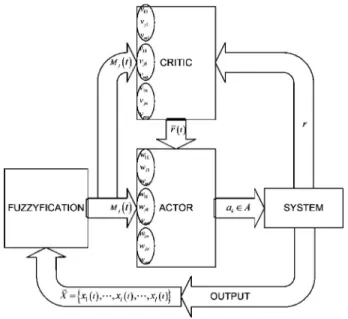
AC methods are a special case of temporal-difference (TD) methods [3], which are formed by two structures. The actor is a separate memory structure to explicitly represent the control policy, which is independent of the value function, whose func-tion is to select the best control acfunc-tions. The critic has the task to estimate the value function, and it is called that way because it criticizes the control actions made by the actor. TD error de-pends also on the reward signal obtained from the environment as a result of the control action. Fig. 1 shows the AC config-uration, whererrepresents the reward signal,r¯is the internal enhanced reinforcement signal, andais the selected action for the current system state.
B. Probabilistic Fuzzy Logic
Probabilistic modeling has proven to be a useful tool in many engineering fields to handle random uncertainties, such as in finance markets [13], and in engineering fields, such as robotic control systems [15], power systems [16], and signal process-ing [17]. As probabilistic methods and fuzzy techniques are complementary to process uncertainties [18], [19], it is a valu-able job to endow the FLS with probabilistic features. The in-tegration of probability theory and fuzzy logic has also been studied in [20].
PFL systems work in a similar way as regular fuzzy-logic systems and encompass all their parts: fuzzification, aggrega-tion, inference, and defuzzification; however, they incorporate probabilistic modeling, which improve the stochastic model-ing capability like in [21], who applied it to solve a function-approximation problem and a control robotic system, showing a better performance than an ordinary FLS under stochastic cir-cumstances. Other PFS applications include classification prob-lems [22] and financial markets analysis [1].
In GPFRL, after an actionak ∈A={a1, a2, . . . , an}, is exe-cuted by the system, the learning agent performs a new observa-tion of the system. This observaobserva-tion is composed by a vector of inputs that inform the agent about external or internal conditions that can have a direct impact on the outcome of a selected action. These inputs are then processed using Gaussian-membership functions according to
Left shoulder:μLi (t) =
1, if xi≤cL
e−(1/2)((xi(t)−cL)/σL)
2
,otherwise Center MFs:μCi (t) =e−(1/2)((xi(t)−cC)/σC)
2
Right shoulder:μRi (t) =
e−(1/2)((xi(t)−cR)/σR)
2
,ifxi≤cR 1,otherwise
(1) where μ{iL ,C ,R} is the firing strength of input xi, i=
{1,2, . . . , l}is the input number,L,C, andRspecify the type of membership function used to evaluate each input,xi is the normalized value of inputi,c{L ,C ,R} is the center value of the Gaussian-membership function, andσ{L ,C ,R} is the standard deviation for the corresponding membership function.
We consider a PFL system composed of a set of following rules.
Rj: Ifx1 isX1h. . . xi isXih. . ., andxl isXlh, theny isa1 with a probability of success ofρj1,. . .,ak with a probability of success ofρj k, andan with a probability of success ofρj n. whereRjis thejth rule of the rule base,Xihis thehth linguistic value for inputi, andh={1,2, . . . , qi}, whereqi is the total number of membership functions for inputxi. Variableydenotes the output of the system, andak is a possible value fory, with
k={1,2, . . . , n}being the action number andnbeing the total number of possible actions that can be executed. The probability of this action to be successful isρj k, wherej={1,2, . . . , m} is the rule number, andmis the total number of rules. These success probabilitiesρj k are the normalization of the s-shaped weights of the actor, evaluated at time stept, and are defined by
ρj k(t) =
S[wj k(t)] n
k= 1S[wj k(t)]
(2) whereSis an s-shaped function given by
S[wj k(t)] = 1
1−e−wj k(t) (3)
andwj k(t)is a real-valued weight that maps rulejwith action
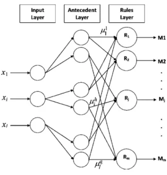
kat a time stept. The FIS structure can be seen in Fig. 2. The total probability of success of performing actionak con-siders the effect of all individual probabilities and combines
Fig. 2. FIS scheme.
them using a weighted average, where Mj are all the conse-quents of the rules, andPk(t)is the probability of success of executing actionak at time stept, which is defined as follows:
Pk(t) = m
j= 1Mj(t)·ρj k(t) m
j= 1Mj(t)
. (4)
Choosing an action merely considering Pk(t) will lead to an exploiting behavior. In order to create a balance, Lee [6] suggested the addition of a noise signal with mean zero and a Gaussian distribution. The use of this signal will force the system into an explorative behavior, where different from optimum actions are selected for all states; thus, a more accurate input– output mapping is created at the cost of learning speed. In order to maximize both accuracy and learning speed, an enhanced noise signal is proposed. This new signal is generated by a stochastic noise generator defined by
ηk =N(0, σk) (5)
whereN is a random-number-generator function with a Gaus-sian distribution, mean zero, and a standard deviationσk, which is defined as follows:
σk = 1
1 +e[2pk(t)]. (6)
The stochastic noise generator uses the prediction of eventual reinforcement pk(t), as shown in (11), as a damping factor in order to compute a new standard deviation. The result is a noise signal, which is more influential at the beginning of the runs, boosting exploration, but quickly becomes less influential as the agent learns, thereby leaving the system with its default exploitation behavior.
The final output will be a weighted combination of all actions and their probabilities, as shown in (7), whereais a vector of
the final outputs
a=
n k= 1
Ak ×(Pk+ηk) (7)
IV. GENERALIZEDPROBABILISTICFUZZY REINFORCEMENTLEARNING
The learning process of a GPFRL is based on an AC RL scheme, where the actor learns the policy function, and the critic learns the value function using the TD method simultaneously. This makes possible to focus on online performance, which involves finding a balance between exploration (of uncharted environment) and exploitation (of the current knowledge).
Formally, the basic RL model consists of the following: 1) a set of environment state observationsO;
2) a set of actionsA;
3) a set of scalar “rewards”r.
In this model, an agent interacts with a stochastic environment at a discrete, low-level time scale. At each discrete time stept, the environment acquires a set of inputsxi∈Xand generates an observationo(t)of the environment. Then, the agent performs and action, which is the result of the weighted combination of all the possible actions ak ∈A, whereA is a discrete set of actions. The action and observation events occur in sequence,
o(t), a(t), o(t+ 1), a(t+ 1), . . .. This succession of actions and observations will be called experience. In this sequence, each event depends only on those preceding it.
The goal in solving a Markov decision process is to find a way of behaving, or policy, which yields a maximal reward [23]. Formally, a policy is defined as a probability distribution for picking actions in each state. For any policyπ:s×A→[0,1] and any states∈S, the value function ofπfor statesis defined as the expected infinite-horizon discounted return froms, given that the agent behaves according toπ
Vπ(s) =Eπ
rt+ 1+γrt+ 2+γ2rt+ 3+· · · |st=s
(8) where γ is a factor between 0 and 1 used to discount future rewards. The objective is to find an optimal policy,π∗, which maximizes the valueVπ(s)of each states. The optimal value function, i.e.,V∗, is the unique value function corresponding to any optimal policy.
RL typically requires an unambiguous representation of states and actions and the existence of a scalar reward function. For a given state, the most traditional of these implementations would take an action, observe a reward, update the value function, and select, as the new control output, the action with the highest expected value in each state (for a greedy-policy evaluation). The updating of the value function is repeated until convergence is achieved. This procedure is usually summarized under policy improvement iterations.
The parameter learning of the GPFRL system includes two parts: the actor-parameter learning and the critic-parameter learning. One feature of the AC learning is that the learning of these two parameters is executed simultaneously.
Given a performance measurementQ(t), and a minimum de-sirable performanceQm in, we define the external reinforcement
signalras follows:
r=
0 ∀Q(t)≥Qm in >0
−1 ∀0≤Q(t)< Qm in. (9)
The internal reinforcement, i.e.,r¯, which is expressed in (10), is calculated using the TD of the value function between suc-cessive time steps and the external reinforcement
¯
rk(t) =r(t) +γpk(t)−pk(t−1) (10) whereγis the discount factor used to determine the proportion of the delay to the future rewards, and the value functionpk(t) is the prediction of eventual reinforcement for actionak and is defined as
pk(t) = m j= 1
Mj(t)·vj k(t) (11)
wherevj kis the critic weight of thejth rule, which is described by (13).
A. Critic Learning
The goal of RL is to adjust correlated parameters in order to maximize the cumulative sum of the future rewards. The role of the critic is to estimate the value function of the policy followed by the actor. The TD error, is the TD of the value function between successive states. The goal of the learning agent is to train the critic to minimize the error-performance index, which is the squared TD errorEk(t), and is described as follows:
Ek(t) = 1 2¯r
2
k(t). (12)
Gradient–descent methods are among the most widely used of all function-approximation methods and are particularly well-suited to RL [24] due to its guaranteed convergence to a local optimum under the usual stochastic approximation conditions. In fact, gradient-based TD learning algorithms that minimizes the error-performance index has been proved convergent in gen-eral settings that includes both on-policy and off-policy learn-ing [25].
Based on the TD error-performance index (12), the weights
vj k of the critic are updated according to equations (13)–(19) through a gradient–descent method and the chain rule [26]
vj k(t+ 1) =vj k(t)−β
∂Ek(t)
∂vj k(t)
. (13)
In (13),0< β <1 is the learning rate,Ek(t)is the error-performance index, andvj k is the vector of the critic weights.
Rewriting (13) using the chain rule, we have
vj k(t+ 1) =vj k(t)−β
∂Ek(t)
∂r¯k(t)
· ∂¯rk(t)
∂pk(t)
· ∂pk(t)
∂vj k(t) (14)
∂Ek(t)
∂r¯k(t)
= ¯rk(t) (15)
∂¯rk(t)
∂pk(t)
=γ (16)
∂pk(t)
∂vj k(t)
=Mj(t) (17)
vj k(t+ 1) =vj k(t)−βγr¯k(t)·Mj(t) (18)
vj k(t+ 1) =vj k(t)−βr¯k(t)·Mj(t). (19) In (19),0< β<1is the new critic learning rate.
B. Actor Learning
The main goal of the actor is to find a mapping between the input and the output of the system that maximizes the perfor-mance of the system by maximizing the total expected reward. We can express the actor value functionλk(t)according to
λk(t) = m j= 1
Mj(t)·ρj k(t). (20) Equation (20) represents a component of a mapping from an m-dimensional input state derived from x(t)∈Rm to a
n-dimensional stateak ∈Rn.
Then, we can express the performance functionFk(t)as
Fk(t) =λk(t)−λk(t−1). (21) Using the gradient–descent method, we define the actor-weight-updating rule as follows:
wj k(t+ 1) =wj k(t)−α
∂Fk(t)
∂wj k(t)
(22) where0< α <1is a positive constant that specifies the learning rate of the weightwj k. Then, applying the chain rule to (22), we have
∂Fk(t)
∂wj k(t)
=∂Fk(t)
∂λk(t) ·
∂λk(t)
∂ρj k(t)·
∂ρj k(t)
∂wj k(t)
(23)
∂Fk(t)
∂wj k(t)
= Mj(t)·ρ2j k(t)·e−wj k(t)
×[ρj k(t)−1]· m j= 1
S[wj k(t)]. (24) Hence, we obtain
wj k(t+ 1) =wj k(t)−α·Mj(t)·ρ2j k(t)
×e−wj k(t)·[ρ
j k(t)−1]· m j= 1
S[wj k(t)] (25) Equation (25) represents the generalized weight-update rule, where0< α <1is the learning rate.
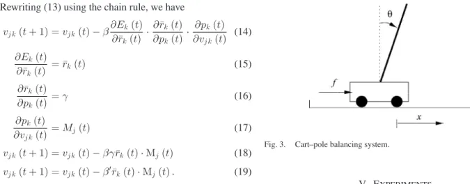
Fig. 3. Cart–pole balancing system.
V. EXPERIMENTS
In this section, we consider a number examples regarding our proposed RL approach. First, we consider the control of a simulated cart–pole system. Second, we consider the control of a dc motor. Third, we consider a complex control problem for mobile-robot navigation.
A. Cart–Pole Balancing Problem
In order to assess the performance of our approach, we use a cart–pole balancing system. This model was used to compare GPFRL (for both discrete and continuous actions) to the original AHC [3], and other related RL methods.
For this case, the membership functions (i.e., centers and standard deviations) and the actions are preselected. The task of the learning algorithm is to learn the probabilities of success of performing each action for every system state.
1) System Description: The cart–pole system, as depicted in Fig. 3, is often used as an example of inherently unstable and dynamic systems to demonstrate both modern and classic control techniques, as well as the learning control techniques of neural networks using supervised learning methods or RL methods. In this problem, a pole is attached to a cart that moves along one dimension. The control tasks is to train the GPFRL to determine the sequence of forces and magnitudes to apply to the cart in order to keep the pole vertically balanced and the cart within the track boundaries for as long as possible without failure. Four state variables are used to describe the system status, and one variable represents the force applied to the cart. These are the displacementxand velocityx˙ of the cart and the angular displacementθand its angular speedθ˙. The action is the forcefto be applied to the cart. A failure occurs when|θ| ≥12◦ or|x| ≥2.4 m. The success is when the pole stays within both these ranges for at least 500 000 time steps.
The dynamics of the cart–pole system are modeled as in (26)–(29), shown at the bottom of the next page, wheregis the acceleration due to gravity,mcis the mass of the cart,mis the mass of the pole,lis the half-pole length,μcis the coefficient of friction of the cart on track, andμp is the coefficient of friction of the pole on the cart. The values used are the same as the ones used in [3], which are as follows.
1) g=−9.8 m/s2 is the acceleration due to the gravity.
2) mc= 1 kgis the mass of the cart. 3) m= 0.1 kgis the mass of the pole.
TABLE I
PARAMETERSUSED FOR THECART–POLERL ALGORITHM
4) l= 0.5 mis the half-pole length.
5) μc= 0.0005is the coefficient of friction of the cart on the track.
6) μp = 0.000002is the coefficient of friction of the pole on the cart.
These equations were simulated by the Euler method using a time step of 20 ms (50 Hz).
One of the important strengths of the proposed model is its ca-pability of capturing and dealing with the uncertainty in the state of the system. In our particular experiment with the cart–pole problem, this may be caused by uncertainty in sensor readings and the nonlinearity inherent to the system.
To avoid the problem generated byx˙ = 0in the simulation study, we use (30), as described in [27]
f =
μNsgn ( ˙x), x˙ = 0
μNsgn (Fx), x˙ = 0. (30) Table I shows the selected parameters for our experiments, whereαis the actor learning rate,β is the critic learning rate,
τ is the time step in seconds, andγis the TD discount factor. The learning rates were selected based on a sequence of exper-iments as shown in the next section. The time step is selected to be equal to the standard learning rate used in similar studies, and the discount factor was selected based on the basic criteria that for values of γ close to zero. The system is almost only concerned with the immediate consequences of its action. For values approaching one, future consequences become a more important factor in determining optimal actions. In RL, we are more concerned in the long-term consequences of the actions; therefore, the selected value forγis chosen to be 0.98.
2) Results: Table II shows the probabilities of success of applying a positive force to the cart for each system state. The probability values that are shown in Table II are the values obtained after a complete learning run. It can be observed that values close to 50% are barely “visited” system states that can ultimately be excluded, which reduces the number of fuzzy rules. This can also be controlled by manipulating the value of the stochastic noise generator, which can be set either to force an exploration behavior, increase the learning time, or force an
TABLE II
PROBABILITIES OFSUCCESS OFAPPLYING APOSITIVEFORCE TO THECART FOR
EACHSYSTEMSTATE
exploitation behavior, which will ensure a fast convergence, but will result in fewer states being visited or “explored.”
We used the pole balancing problem with the only purpose of comparing our GPFRL approach to other RL methods. Sut-ton and Barto [3] proposed an AC learning method, which is called AHC, and was based on two single-layer neural networks aimed to control an inverted pendulum by performing a dis-cretization of a 4-D continuous input space, using a partition of these variables with no overlapping regions and with not any generalization between subspaces. Each of these regions con-stitutes a box, and a Boolean vector indicates in which box the system is. Based on this principle, the parameters that model the functions are simply stored in an associated vector, thereby providing a weighting scheme. For large and continuous state spaces, this representation is intractable (curse of dimensional-ity). Therefore, some form of generalization must be incorpo-rated in the state representation. AHC algorithms are good at tackling credit-assignment problems by making use of the critic and eligibility traces. In this approach, correlations between state variables were difficult to embody into the algorithm, the control structure was excessively complex, and suitable results for complex and uncertain systems could not be obtained.
Anderson [4] further realized the balancing control for an inverted pendulum under a nondiscrete state by an AHC al-gorithm, which is based on two feed-forward neural networks. In this work, Anderson proposed a divided state space into fi-nite numbers of subspaces with no generalization between sub-spaces. Therefore, for complex, and uncertain systems a suitable division results could not be obtained, correlations between state variables were difficult to embody into the algorithm, the con-trol structure was excessively complex, and the learning process took too many trials for learning.
Lee [6] proposed a self-learning rule-based controller, which is a direct extension of the AHC described in [3] using a fuzzy
¨
θ=
gsinθ+ cosθ
(−f−mlθ˙2sinθ+μ
csgn ( ˙x)/(mc+m)
−(μpθ/ml˙ )
l[(4/3)−(mcos2θ/(m
c+m)]
(26)
¨
x=
f+ml
˙
θ2sinθ−θ¨cosθ−μ
csgn ( ˙x)
mc+m
(27)
θ(t+ 1) =θ(t) + Δ ˙θ(t) (28)
partition rather than the box system to code the state and two single-layer neural networks. Lee’s approach is capable of work-ing on both continues inputs (i.e., states) and outputs (i.e., ac-tions). However, the main drawback of this implementation is that as a difference with the classic implementation in which the weight-updating process act as a quality modification due to the bang–bang action characteristic (the resulting action is only determined by the sign of the weight), in Lee’s, it acts as an action modificator. The internal reinforcement is only able to inform about the improvement of the performance, which is not informative enough to allow an action modification.
The GARIC architecture [5] is an extension of ARIC [28], and is a learning method based on AHC. It is used to tune the linguistic label values of the fuzzy-controller rule base. This rule base is previously designed manually or with another automatic method. The critic is implemented with a neural network and the actor is actually an implementation of a fuzzy-inference system (FIS). The critic learning is classical, but the actor learning, like the one by Lee [6], acts directly on action magnitudes. Then, GARIC-Q [29] extends GARIC to derive a better controller using a competition between a society of agents (operating by GARIC), each including a rule base, and at the top level, it uses fuzzy Q-learning (FQL) to select the best agent at each step. GARIC belong to a category of off-line training systems (a dataset is required beforehand). Moreover, they do not have a capability of structure learning and it needs a large number of trials to be tuned. A few years later, Zarandiet al.[9] modified this approach in order to handle vagueness in the control states. This new approach shows an improvement in the learning speed, but did not solve the main drawbacks of the GARIC architecture. While the approach presented by Zarandiet al. [9] is able to handle vagueness on the input states, it fails to generalize it in order to handle uncertainty.
In supervised learning, precise training is usually not avail-able and is expensive. To overcome this problem, Lin and Lee [30], [31] proposed an RNN-FLCS, which consists of two fuzzy neural networks (FNNs); one performs a fuzzy-neural controller (i.e., actor), and the other stands for a fuzzy-neural evaluator (i.e., critic). Moreover, the evaluator network provides internal reinforcement signals to the action network to reduce the uncertainty faced by the latter network. In this scheme, us-ing two networks makes the scheme relatively complex and its computational demand heavy. The RNN-FLCS can find proper network structure and parameters simultaneously and dynam-ically. Although the topology structure and the parameters of the networks can be tuned online simultaneously, the num-ber and configuration of memnum-bership functions for each in-put and outin-put variable have to be decided by an expert in advance.
Lin [12] proposed an FALCON-RL, which is based on the FALCON algorithm [32]. The FALCON-RL is a type of FNN-based RL system (like ARIC, GARIC, and RNN-FLCS) that uses two separate five-layer perceptron networks to fulfill the functions of actor and critic networks. With this approach, the topology structure and the parameters of the networks can be tuned online simultaneously, but the number and configuration of membership functions for each input and output variable
have to be decided by an expert in advance. In addition, the architecture of the system is complex.
Jouffe [10] investigated the continuous and discrete actions by designing two RL methods with function-approximation im-plemented using FIS. These two methods, i.e., FACL and FQL, are both based on dynamic-planning theory while making use of eligibility traces to enhance the speed of learning. These two methods merely tuned the parameters of the consequent part of a FIS by using reinforcement signals received from the envi-ronment, while the premise part of the FIS was fixed during the learning process. Therefore, they could not realize the adaptive establishment of a rule base, limiting its learning performance. Furthermore, FACL and FQL were both based on dynamic-programming principles; therefore, system stability and perfor-mance could not be guaranteed.
Another approach based on function approximation is the RLAFC method, which was proposed by Lin [11]; here, the action-generating element is a fuzzy approximator with a set of tunable parameters; moreover, Lin [11] proposed a tuning algorithm derived from the Lyapunov stability theory in order to guarantee both tracking performance and stability. Again in this approach, the number and configuration of the membership functions for each input and output variable have to be decided by an expert in advance. It also presents the highest number of fuzzy rules of our studies and a very complex structure.
In order to solve the curse of the dimensionality problem, Wang et al.[14] proposed a new FACRLN based on a fuzzy-radial basis function (FRBF) neural network. The FACRLN used a four-layer FRBF neural network that is used to approximate both the action value function of the actor and the state-value function of the critic simultaneously. Moreover, the FRBF net-work is able to adjust its structure and parameters in an adaptive way according to the complexity of the task and the progress in learning. While the FACRLN architecture shows an excellent learning rate, it fails to capture and handle the system input uncertainties while presenting a very complex structure.
The detailed comparison is presented in Table III, from which we see that our GPFRL system required the smallest number of trials and had the least angular deviation. The data presented in Table III has been extracted from the referenced publications. Fields where information was not available are marked as N/I, and fields with information not applicable are marked as N/A.
For this experiment, 100 runs were performed with a run ending when a successful input/output mapping was found or a failure occurred. A failure run is said to occur if no successful controller is found after 500 trials. The number of pole balance trials was measured for each run and their statistical results are shown in Fig. 4. The minimum and the maximum number of trials over these 100 runs were 2 and 10, and the average number of trials was 3.33 with only four runs failing to learn. It is also to be noted that there are 59 runs that took between three and four trials in order to correctly learn the probability values of the GPFRL controller.
In order to select an appropriate value for the learning rate, a value that minimizes the number of trials required for learning but, at the same time, minimizes the number of no-learning runs (a run in which the system executed 100 or more trials
TABLE III
LEARNINGMETHODCOMPARISON ON THECART–POLEPROBLEM
Fig. 4. Trials distribution over 100 runs.
Fig. 5. Actor learning rate; alpha versus number of failed runs.
without success), a set of tests were performed and their results are depicted in Figs. 5–8. In there graphs, the solid black line represents the actual results, while the dashed line is a second-order polynomial trend line. In Figs. 5 and 6, it can be observed that the value of alpha does not have a direct impact on the number of failed runs (which is in average 10%). It has, however, more impact on the learning speed, where there is no significance increase on the learning speed for a value higher than 45. For these tests, the program executed the learning algorithm 22 times, each time consisting of 100 runs, from which the average was taken.
For the second set of tests, the values of beta were changed (see Figs. 7 and 8) while keeping alpha at 45. It can be observed that there is no significant change in the amount of failed runs for beta values under 0.000032. With beta values over this, the number of nonlearning runs increases quickly. Contrarily, for values of beta below 0.000032, there is no major increase on the learning rate.
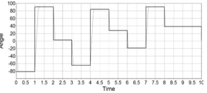
The results of one of the successful runs are shown in Figs. 9–12, where the cart position, i.e.,x(see Fig. 9), the pole angle,
Fig. 6. Actor learning rate; alpha versus number of trials for learning.
Fig. 7. Critic learning rate; beta versus number of failed runs.
Fig. 8. Critic learning rate; beta versus number of trials for learning.
i.e.,θ(see Fig. 10), the control force, i.e.,f (see Fig. 11), and the stochastic noise, i.e.,η(see Fig. 12) are presented.
Fig. 9 depicts the cart position in meters over the first 600 s of a run, after the system has learned an appropriate policy. It can be observed that the cart remains within the re-quired boundaries with an offset of approximately of –0.8 m as the system is expected to learn how to keep the cart within a range and not to set it at a determinate position.
Fig. 10 shows the pole angle in degrees, which is captured in the last trial of a successful run. The average peak-to-peak
Fig. 9. Cart position at the end of a successful learning run.
Fig. 10. Pole angle at the end of a successful learning run.
Fig. 11. Applied force at the end of a successful learning run.
Fig. 12. Stochastic noise.
angle was calculated to be around 0.4◦, thus outperforming the performance of previous works. In addition, it can be noted that this value oscillates around an angle of 0◦, as this can be considered the most-stable position due to the effect of gravity. Therefore, it can be said that the system successfully learns how to keep the pole around this value.
Fig. 11 shows the generated forces that push the cart in either direction. This generated force is a continuous value that ranges from 0 to 10 and is a function of the combined probability of success for each visited state. As expected, this force is thrilled around 0, thus resulting in no average motion of the cart in either direction and, thus, keeping it within the required boundaries.
Fig. 13. Motor with load attached.
Finally, Fig. 12 shows the stochastically generated noise, which is used to add exploration/exploitation behavior to the system. This noise is generated by the stochastic noise genera-tor described by (5) and (6). In this case, a small average value indicates that preference is given to exploitation rather than ex-ploration behavior, as expected at the end of a learning trial. The range of the generated noise depends on the value of the stan-dard deviation σk, which varies over the learning phase, thus giving a higher priority to exploration at the beginning of the learning and an increased priority to exploitation as the value of the prediction of eventual reinforcementpk(t)increases.
B. DC-Motor Control
The system in this experiment consists of a dc motor with a gear-head reduction box. Attached to the output shaft is a lever (which is considered to have no weight) of length “L” and at the end of this a weight “w.” The starting point (at which the angle of the output shaft is considered to be at angle 0) is when the lever is in vertical position, with the rotational axis (motor shaft) over the weight; therefore, the motor shaft is exerting no torque. Fig. 13 shows the motor arrangement in its final position (refer-ence of 90◦).
1) Control-Signal Generation: For the present approach, let us assume that there are only two possible actions to take: direct or reverse voltage, i.e., the controller will apply either 24 or –24 V to the motor, thereby spinning it clockwise or counter-clockwise. At high commutation speeds, the applied signal will have the form of a pulsewidth-modulated (PWM) signal whose duty cycle controls the direction and speed of rotation of the motor.
The selection of either of the actions, which are described above, will depend on the probability of success of the current state of the system. The goal of the system is to learn this probability through RL.
The inputs to the controller are the error and the rate of change of the error as it is commonly used in fuzzy controllers.
2) Failure Detection: For the RL algorithm to perform, an adequate definition of failure is critical. Deciding when the sys-tem has failed and defining its bias is not always an easy task. It can be as simple as analyzing the state of the system, like in the case of the classic cart–pole problem [3], or it can get
Fig. 14. Membership functions for the error input.
Fig. 15. Membership functions for the rate of change of error. TABLE IV
COEFFICIENTVALUES FOR THERL ALGORITHM
complicated if the agent needs to analyze an external object. For example, in a welding machine, a positive reinforcement can be attributed if the weld has been successful or a failure if it has not.
The proposed system continuously analyses the performance of the controller by computing the time integral of absolute error (IAE), as specified by
IAE=
∞
0
|e(t)|dt. (31)
In (31),e(t)is the difference between the reference position and the actual motor position (i.e., system error). The IAE is computed at every time step and is compared with a selectable threshold value. A control system failure is considered when the measured IAE is over the stated threshold, thus generating a negative reinforcement and resetting the system to start a new cycle.
The IAE criterion will penalize a response that has errors that persist for a long time, thus making the agent learn to reduce the overshoot and, furthermore, the steady-state error.
Furthermore, the IAE criterion will be used to evaluate the system performance quantitatively and compare it against other methods.
3) System Configuration: The membership functions used to fuzzify the inputs are depicted in Figs. 14 and 15. Their param-eters were selected based on experience, and their optimization goes beyond the scope of this paper.
The RL agent requires some parameters to be defined. Table IV shows the values selected by the following selection principles [14].
TABLE V
PROBABILITYMATRIXSHOWING THEPROBABILITY OFSUCCESS OF
PERFORMINGACTION A1FOREVERYRULE
First, by adjusting the discount factor γ, we were able to control the extent to which the learning system is concerned with long-term versus short-term consequences of its own actions. In the limit, whenγ= 0, the system is myopic in the sense that it is only concerned with immediate consequences of its action. As γ approaches 1, future costs become more important in determining optimal actions. Because we were rather concerned with long-term consequences of its actions, the discount factor had to be large, i.e., we setγ= 0.95.
Second, if a learning rate is small, the learning speed is slow. In contrast, if a learning rate is large, the learning speed is fast, but oscillation occurs easily. Therefore, we chose small learning rates to avoid oscillation, such asα=7 andβ=1.
4) Results: The program developed searches for possible probability values and adjusts the corresponding one accord-ingly. It runs in two phases: the first one with a positive reference value and the second one with a complementary one; hence, it will learn all the probability values of the rule matrix. For the following case, we consider a test as a set of trials performed by the agent until the probabilities of success are learned so that the system does not fail. A trial is defined as the period in which a new policy is tested by the actor. If a failure occurs, then the policy is updated, and a new trial is started.
After performing 20 tests, the agent was able to learn the probability values in an average of four trials. The values for each probability after every test were observed to be, in every case, similar to the ones shown in Table V, thus indicating an effective convergence.
As an example, from Table V, we have the following: “IFe=LN AND˙e=SN, THENy=A1withp1=0.38 andy=
A2with p2=0.62.”
Then, the final action is evaluated using (4), and the final probabilities of performing actionA1 andA2 are calculated. Finally, the action chosen will be the action with the highest probability of success.
The following plots were drawn after the learning was complete.
Fig. 16 shows the motor angle when a random step signal is used as reference, and Fig. 17 is a zoomed view of the error in a steady state.
Fig. 18 illustrates the learning process. The system starts 90◦ apart from the reference. After four trials, the agent config-ured the fuzzy-logic rules so that the error rapidly converged to zero.
Fig. 16. Motor response to a random step reference. The solid black line represents the reference signal, and the gray one represents the current motor angle.
Fig. 17. Motor error in steady state after all trials are performed and the system has learned the correct consequent probabilities.
Fig. 18. Trials for learning.
C. Mobile-Robot Obstacle Avoidance
The two most important topics in mobile-robot design are planning and control. Both of them can be considered as a utility-optimization problem, in which a robot seeks to maximize the expected utility (performance) under uncertainty [33].
While recent learning techniques have been successfully applied to the problem of robot control under uncertainty [34]–[36], they typically assume a known (and stationary) model of the environment. In this section, we study the problem of finding an optimal policy to control a robot in a stochastic and partially observable domain, where the model is not perfectly known and may change over time. We consider that a proba-bilistic approach is a strong solution not only to the navigation problem but to a large range of robot problems that involves sensing and interacting with the real world as well. However, few control algorithms make use of full probabilistic solutions,
Fig. 19. (Left) IR sensor distribution in the Khepera III robot. (Right) Khepera III robot.
and as a consequence, robot control can become increasingly fragile as the system’s perceptual and state uncertainty increase. RL enables an autonomous mobile robot interacting with a stochastic environment to select the optimal actions based on its self-learning mechanism. Two credit-assignment problems should be addressed at the same time in RL algorithms, i.e., structural- and temporal-assignment problems. The autonomous mobile robot should explore various combinations of state-action patterns to resolve these problems.
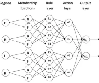
In our third experiment, the GPFRL algorithm was imple-mented on a Khepera III mobile robot (see Fig. 19) in order to learn a mapping that will enable itself to avoid obstacles. For this case, four active learning agents were implemented to read information from IR distance sensors and learn the probabilities of success for the preselected actions.
1) Input Stage: The Khepera III robot is equipped with nine IR sensors distributed around it (see Fig. 19). For every time step, an observationot∈Oof the system state is taken. It consists of a sensor readingxk(t), k= 1,2, . . . , l, wherelis the number of sensors, andxk is the measured distance at sensork. The value ofxkis inversely proportional to the distance between the sensor and the obstacles, wherexk(t) = 1represents adistance of zero between sensorkand the obstacle, andxk(t) = 0corresponds to an infinite distance.
The input stage is composed by two layers: the input layer and the regions layer (see Fig. 20), which shows how the nine signals acquired from the sensors are grouped inside the network into the four predefined regions. In this figure, lines L1 and L2 are two of the four orthogonal lines.
In order to avoid the dimensionality problem, a clustering approach was used. Signals from sensors 2, 3, 4, 5, 6, and 7 are averaged (weighted average using the angle with the orthogonal as a weight). They inform about obstacles in the front. Signals from sensors 1, 8, and 9 are grouped together and averaged. They inform about obstacles behind the robot. Another clustering procedure is applied to signals coming from sensors 1, 2, 3, and 4, which inform about obstacles to the right, and IR sensors 5, 6, 7, and 8, which inform about obstacles to the left.
In (32), xR
k is the result of the averaging function, where
R, R={1,2,3,4}represents the evaluated region: front, back, left, and right,IRs is the input value of sensors, andθRs is the
Fig. 20. Clustering of IR inputs into four regions. It is to be noted that some sensors contribute to more than one region.
Fig. 21. Membership functions for the averaged inputs. TABLE VI
CENTER ANDSTANDARDDEVIATION FOR ALLMEMBERSHIPFUNCTIONS
angle between the sensor orientation and the orthogonal lineR xRk =
s s=s1
90−θR
s
×IRs s
s=s1(90−θ
R s)
. (32)
The signals from the averaging process are then fuzzified us-ing Gaussian-membership functions, as specified in (33). Only two membership functions (a left shouldered and a right shoul-dered) with linguistic names of “far” and “near” were used to evaluate each input. These membership functions are depicted in Fig. 21 and defined according to
Far:μLk (t) =
1, if xk ≤cL
e−(1/2)((xk(t)−cL)/σL)
2
, otherwise Near:μRk (t) =
e−(1/2)((xk(t)−cR)/σR)
2
, ifxk ≤cR
1, otherwise .
(33) The center and standard deviation values used in (33) were manually adjusted for this particular case, and their values are shown in Table VI.
2) Rules Stage: In this layer, the number of nodes is the result of the combination of the number of membership functions
Fig. 22. Controller structure.
that each region has and is divided in two subgroups. Each one of them triggers two antagonistic actions and is tuned by independent learning agents. Fig. 22 shows the interconnection between the rules layer and the rest of the network.
3) Output Stage: Finally, the output stage consists of an action-selection algorithm. We describe action Aj, j = 1,2, . . . , m, wheremis the maximum number of actions. For this particular case, there are following four possible actions:
1) A1 =go forward; 2) A2 =go backwards; 3) A3 =turn left;
4) A4 =turn right.
These actions are expressed as a vector, where each term represents a relative wheel motion, which are coded as forward: (1, 1), backward: (–1, –1), turn right: (1, –1), and turn left: (–1, 1). The velocity is then computed using
v=
m j= 1
Aj ×Pj (34)
where v= (v1, v2), and each of its terms represent the
nor-malized speed of each of the wheels. Evaluating (34) on both maximum and minimum cases ofPj, we obtain
vm ax = (2,2). (35)
In order not to saturate the speed controller of the robot’s wheels, we express the velocity for each wheel as
VL /R = 1
2Vm ax×v1/2 (36) In (36),Vm ax is the maximum allowed speed for the wheels of the robot, andVL /R is the final speed commanded to each wheel.
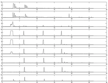
4) Results: For this experiment, we implemented our algo-rithm in a Khepera III robot. Fig. 23 depicts the distance in-formation coming from the IR sensors. The signal spikes indi-cate obstacle detection (wall). A flat top in the spikes indiindi-cates that saturation was produced due to a crash against an obsta-cle. Fig. 24 shows the error-performance indexE(t). After the
Fig. 23. Khepera III sensor reading for 30 s trial.
Fig. 24. Internal reinforcementE(t).
learning process, the robot avoids all the obstacles successfully. In our experiments, the average learning time was around 18 s, as can be seen in Fig. 23, where saturation stops occurring, and in Fig. 24, where the error-performance index E(t)becomes minimum after approximately 18 s.
VI. CONCLUSION
RL has the ability to make use of sparse information from the environment to guide the learning process. It has been widely used in many applications.
In order to apply RL to systems working under uncertain con-ditions, and based on the successful application of PFL systems to situation presenting uncertainties, new probabilistic fuzzy-RL has been proposed in our investigation.
We introduce the capability of RL of being able to approxi-mate both the action function of the actor and the value function of the critic simultaneously into a PFL system reducing the de-mand for storage space from the learning system and avoiding repeated computations for the outputs of the rule units. There-fore, this probabilistic fuzzy-RL system is much simpler than many other RL systems.
Furthermore, the GPFRL decision process is not determined entirely by the policy; it is rather based on a weighted
com-bination action-probability, thereby resulting in effective risk-avoidance behavior.
Three different experimental studies concerning the cart–pole balancing control, a dc-motor controller, and a Khepera III mo-bile robot, demonstrate the validity, performance, and robustness of the proposed GPFRL, with its advantages for generalization, a simple control structure, and a high learning efficiency when interacting with stochastic environments.
REFERENCES
[1] J. van den Berget al., “Financial markets analysis by using a probabilis-tic fuzzy modelling approach,” Int. J. Approx. Reason., vol. 35, no. 3, pp. 291–305, 2004.
[2] R. E. Bellman,Dynamic Programming. Princeton, NJ: Princeton Univ. Press, 1957.
[3] A. G. Bartoet al., “Neuron-like adaptive elements that can solve difficult learning control problems,”IEEE Trans. Syst., Man, Cybern., vol. SMC-13, no. 5, pp. 835–846, 1983.
[4] C. W. Anderson, “Learning to control an inverted pendulum using neural networks,” IEEE Control Syst. Mag., vol. 9, no. 3, pp. 31–37, Apr. 1989. [5] H. R. Berenji and P. Khedkar, “Learning and tuning fuzzy logic controllers through reinforcements,”IEEE Trans. Neural Netw., vol. 3, no. 5, pp. 724– 740, Sep. 1992.
[6] C.-C. Lee, “A self-learning rule-based controller employing approximate reasoning and neural net concept,” Int. J. Intell. Syst., vol. 6, no. 1, pp. 71–93, 1991.
[7] C.-T. Lin and C. S. G. Lee, “Reinforcement structure/parameter learning for neural-network-based fuzzy logic control systems,” presented at the IEEE Int. Conf. Fuzzy Syst., San Francisco, CA, 1993.
[8] C.-T. Lin, “A neural fuzzy control system with structure and parameter learning,” Fuzzy Sets Syst., vol. 70, no. 2/3, pp. 183–212, Mar. 1995. [9] M. H. F. Zarandiet al., “Reinforcement learning for fuzzy control with
linguistic states,” J. Uncertain Syst., vol. 2, pp. 54–66, Oct. 2008. [10] L. Jouffe, “Fuzzy inference system learning by reinforcement methods,”
IEEE Trans. Syst., Man, Cybern., vol. 28, no. 3, pp. 238–255, Aug. 1998. [11] C.-K. Lin, “A reinforcement learning adaptive fuzzy controller for robots,”
Fuzzy Sets Syst., vol. 137, no. 1, pp. 339–352, Aug. 2003.
[12] C.-J. Lin and C.-T. Lin, “Reinforcement learning for an ART-based fuzzy adaptive learning control network,” IEEE Trans. Neural Netw., vol. 7, no. 3, pp. 709–731, May 1996.
[13] R. J. Almeida and U. Kaymak, “Probabilistic fuzzy systems in value-at-risk estimation,” Int. J. Intell. Syst. Account., Finance Manag., vol. 16, no. 1/2, pp. 49–70, 2009.
[14] X.-S. Wanget al., “A fuzzy actor–critic reinforcement learning network,” Inf. Sci., vol. 177, no. 18, pp. 3764–3781, Sep. 2007.
[15] K. P. Valavanis and G. N. Saridis, “Probabilistic modelling of intelligent robotic systems,”IEEE Trans. Robot. Autom., vol. 7, no. 1, pp. 164–171, Feb. 1991.
[16] J. C. Pidreet al., “Probabilistic model for mechanical power fluctuations in asynchronous wind parks,” IEEE Trans. Power Syst., vol. 18, no. 2, pp. 761–768, May 2003.
[17] H. Deshuang and M. Songde, “A new radial basis probabilistic neural network model,” presented at the Int. Conf. Signal Processing, Beijing, China, 1996.
[18] L. A. Zadeh, “Probability theory and fuzzy logic are complementary rather than competitive,”Technometrics, vol. 37, no. 3, pp. 271–276, Aug. 1995. [19] M. Laviolette and J. W. Seaman, “Unity and diversity of fuzziness-from a probability viewpoint,”IEEE Trans. Fuzzy Syst., vol. 2, no. 1, pp. 38–42, Feb. 1994.
[20] P. Liang and F. Song, “What does a probabilistic interpretation of fuzzy sets mean?,” IEEE Trans. Fuzzy Syst., vol. 4, no. 2, pp. 200–205, May 1996.
[21] Z. Liu and H.-X. Li, “A probabilistic fuzzy logic system for modelling and control,” IEEE Trans. Fuzzy Syst., vol. 13, no. 6, pp. 848–859, Dec. 2005.
[22] J. v. d. Berg et al., “Fuzzy classification using probability-based rule weighting,” inProc. IEEE Int. Conf. Fuzzy Syst., Honolulu, HI, 2002, pp. 991–996.
[23] F. Laviolette and S. Zhioua, “Testing stochastic processes through re-inforcement learning,” presented at the Workshop Testing Deployable Learn. Decision Syst., Vancouver, BC, Canada, 2006.
[24] C. Baird, “Reinforcement learning through gradient descent,” Ph.D. dis-sertation, School of Comput. Sci., Carnegie Mellon Univ., Pittsburgh, PA, 1999.
[25] R. S. Suttonet al., “Fast gradient-descent methods for temporal-difference learning with linear function approximation,” inProc. 26th Int. Conf. Mach. Learn., Montreal, QC, Canada, 2009, pp. 993–1000.
[26] L. Baird and A. Moore, “Gradient descent for general reinforcement learn-ing,” inProc. Adv. Neural Inf. Process. Syst. II, 1999, pp. 968–974. [27] H. Yuet al., “Tracking control of a peddulum-driven cart–pole
under-actuated system,” presented at the IEEE Int. Conf. Syst., Man, Cybern., Montreal, QC, Canada, 2007.
[28] H. R. Berenji, “Refinement of approximate reasoning-based controllers by reinforcement learning,” presented at the 8th Int. Workshop Mach. Learn., San Francisco, CA, 1991.
[29] H. R. Berenji, “Fuzzy Q-learning for generalization of reinforcement learning,” presented at the 5th IEEE Int. Conf. Fuzzy Syst., New Orleans, LA, 1996.
[30] C.-T. Lin and C. S. G. Lee, “Reinforcement structure/parameter learning for neural-network-based fuzzy logic control systems,”IEEE Trans. Fuzzy Syst., vol. 2, no. 1, pp. 46–63, Feb. 1994.
[31] C.-T. Lin and C. S. G. Lee, “Neural-network-based fuzzy logic control and decision system,” IEEE Trans. Comput., vol. 40, no. 12, pp. 1320–1336, Dec. 1991.
[32] C.-T. Linet al., “Fuzzy adaptive learning control network with on-line neural learning,” Fuzzy Sets Syst., vol. 71, no. 1, pp. 25–45, Apr. 1995. [33] S. Thrun. (2000) Probabilistic algorithms in robotics.AI Mag.
[34] J. Pineau, “Point-based value iteration: An any time algorithm for POMDPs,” presented at the Int. Joint Conf. Artif. Intell., Acapulco, Mexico, 2003.
[35] P. Poupart and C. Boutilier, “VDCBPI: An approximate scalable algorithm for large POMDPs,” presented at the Advances Neural Inform. Process. Syst., Vancouver, BC, Canada, 2004.
[36] N. Royet al., “Finding approximate POMDP solutions through belief compression,”J. Artif. Intell. Res., vol. 23, no. 1, pp. 1–40, Jan. 2005.
William M. Hinojosareceived the B.Sc. degree in science and engineering, with a major in electronic engineering, the Engineer degree in electrical and electronics, with a major in industrial control, from the Pontificia Universidad Cat´olica del Per´u, Lima, Peru, in 2002 and 2003, respectively, and the M.Sc. degree in robotics and automation in 2006 from The University of Salford, Salford, Greater Manchester, U.K., where he is currently working toward the Ph.D. degree in advanced robotics.
Since September 2003, he has been with the Cen-ter for Advanced Robotics, School of Computing, Science, and Engineering, The University of Salford. Since 2007, he has been a Lecturer in mobile robotics with the University of Salford and the ´Ecole Sup´erieure des Technologies In-dustrielles Avanc´ees, Biarritz, France. He has authored or coauthored a book chapter forHumanoid Robots(InTech, 2009). His current research interests are fuzzy systems, neural networks, intelligent control, cognition, reinforcement learning, and mobile robotics.
Mr. Hinojosa is member of the European Network for the Advancement of Artificial Cognitive Systems, Interaction, and Robotics.
Samia Nefti(M’04) received the M.Sc. degree in electrical engineering, the D.E.A. degree in indus-trial informatics, and the Ph.D. degree in robotics and artificial intelligence from the University of Paris XII, Paris, France, in 1992, 1994, and 1998, respec-tively.
In November 1999, she joined the Liverpool Uni-versity, Liverpool, U.K., as a Senior Research Fellow engaged with the European Research Project Occu-pational Therapy Internet School. Afterwards, she was involved in several projects with the European and U.K. Engineering and Physical Sciences Research Council, where she was concerned mainly with model-based predictive control, modeling, and swarm optimization and decision making. She is currently an Associate Professor of computational intelligence and robotics with the School of Computing Science and Engineering, The University of Salford, Greater Manchester, U.K. Her cur-rent research interests include fuzzy- and neural-fuzzy clustering, neurofuzzy modeling, and cognitive behavior modeling in the area of robotics.
Mrs. Nefti is a Full Member of the Informatics Research Institute, a Char-tered Member of the British Computer Society, and a member of the IEEE Computer Society. She is a member of the international program committees of several conferences and is an active member of the European Network for the Advancement of Artificial Cognition Systems.
Uzay Kaymak(S’94–M’98) received the M.Sc. de-gree in electrical engineering, the Dede-gree of Char-tered Designer in information technology, and the Ph.D. degree in control engineering from the Delft University of Technology, Delft, The Netherlands, in 1992, 1995, and 1998, respectively.
From 1997 to 2000, he was a Reservoir Engineer with Shell International Exploration and Production. He is currently a Professor of economics and com-puter science with the Econometric Institute, Erasmus University, Rotterdam, The Netherlands.