Flow over Triangular Side Weir

(1)

M. Ghodsian 1

In this paper, the hydraulic characteristics of a sharp crested triangular side weir have been experimentally studied. It was found that the DeMarchi coecient of discharge for a sharp crested triangular side weir in subcritical ow is related to the main channel Froude number, the apex angle of weir and ratio of weir height to upstream depth of ow. Suitable equations for discharge coecient are also obtained.

INTRODUCTION

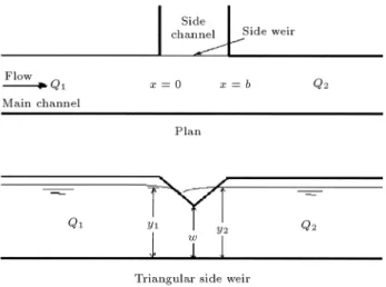
A side weir is an overow and metering diversion structure set into the side of a channel with the purpose of allowing part of the liquid to spill over the side, if the surface of the ow in the channel rise above the weir crest. Side weirs are typically used in irrigation, land drainage, urban sewage systems and sanitary engineering and are also widely used for storm relief, as well as head regulators of distributaries.

The ow over a side weir is a typical case of spatially varied ow with decreasing discharge. The discharge over the side weir is aected by the main channel velocity. Like normal weirs, side weirs may be of dierent shapes (i.e., rectangular, triangular, trapezoidal etc.). Further, side weirs may be made sharp or broad crested. Sharp crested rectangular side weirs have been studied extensively by many investigators 1-15]. It is obvious that almost all the investigators have studied the hydraulic characteristics of rectangular side weirs and less attention has been given to the behavior of ow over triangular side weirs. Kumar and Pathak 16] related the discharge coecient of a triangular side weir to approach Froude number and apex angle of the weir.

In this paper, experimental results on sharp crested triangular side weirs with apex angles of 30, 60, 90 and 120 degrees, respectively, are reported. New equations for the discharge coecient are introduced. It was found that the discharge coecient, in addition to approach Froude number, is a function of apex angle and ratio of weir height to upstream depth of ow. The 1. Department of Civil Engineering, Tarbiat Modarres

Uni-versity, Tehran, I.R. Iran.

experiments were restricted to subcritical ow in the main channel and free ow in the side channel.

BASIC THEORY

The ow over a side weir is a typical case of spatially varied ow with decreasing discharge. The energy equation is commonly used for deriving the governing equation for the ow over a side weir. The general dierential equation of spatially varied ow along a side weir (Figure 1) with decreasing discharge, was given by Henderson as 17]:

dy dx

=S 0

;Sf;gAQdQ 2dx 1;

Q2T

gA3

(1)

in whichy= depth of ow,x= distance along side weir from upstream end, S

0 = main channel slope, Sf =

(2)

friction slope, = kinetic energy correction factor, Q= discharge in channel,dQ=dx= discharge per unit length of side weir,g= acceleration due to gravity,A= cross-sectional area of ow and T = top width of the channel section.

For a horizontal (S

0 = 0) prismatic rectangular main channel, assuming the kinetic energy correction factoras unity and neglecting friction losses (Sf = 0), Equation 1 is simplied as:

dy dx = Qy gB 2 y 3 ;Q 2 ; dQ dx (2)

in whichB is the width of main channel.

The discharge per unit length of a triangular side weir is calculated by the following equation, as presented by Kumar and Pathak 16]:

dQ dx

=; 4 15Cm

p

2g(y;w) 1:5

(3)

in which Cm is the side weir discharge coecient, known as the DeMarchi coecient of discharge andw is the side weir apex height.

By assuming that the specic energy, E, is con-stant along the length of the side weir, the discharge in the main channel,Q, is given by:

Q=By p

2g(E;y): (4)

Combining Equations 2 to 4, one obtains: dy

dx

= 8Cm 15B

(E;y)(y;w) 3

0:5 3y;2E

: (5)

Integrating between the limitsx = 0 andx =b 1 (i.e., sections 1 and 2 in Figure 1) and designating the two sections by suxes 1 and 2, respectively, one gets:

b 1=

x 2

;x 1= 15

B 4Cm

( 2

; 1)

(6)

in which b

1 is the distance between sections 1 and 2 along the side weir andis the DeMarchi varied ow function, rst derived by DeMarchi 17] as:

= 2 E;3w E;w

E;y y;w

0:5

;3sin ;1

E;y E;w

0:5

: (7) Equations 6 and 7 can be combined in the form of:

4b 1

Cm 15B

= 2E;3w E;w

"

E;y 2 y

2 ;w

0:5

;

E;y 1 y

1 ;w

0:5

#

;3 "

sin;1

E;y 2 E;w

0:5 ;sin

;1

E;y 1 E;w

0:5 #

(8)

in which y 1 and

y

2 are the depth of ow for sec-tions 1 and 2, respectively (Figure 1). Equasec-tions 4 and 8 can be used to determine the discharge over the side weir. Knowing the upstream condition (Q

1 and E

1), channel and weir geometry (Bb

1

wand apex angle) and Cm, solve fory

2 using Equation 8, then nd Q

2 using Equation 4. The discharge over the side weir, Qs, is determined by:

Qs=Q 1

;Q 2

(9)

in which Q 1 and

Q

2 are the discharges at sections 1 and 2 in the main channel, respectively. The values of Cm can be calculated from measured values of depth and discharge at sections 1 and 2, for a side weir with known geometry.

EXPERIMENTAL SETUP AND

PROCEDURE

The experiments were conducted using a prismatic, horizontal channel. The main channel was 9.0 m long, 0.5 m wide and 0.5 m deep. The main and side channel were made of brick masonry and plastered with cement. A suitable sluice gate was provided at the downstream end of the main channel for maintaining the desired depth of ow in this channel. The side channel was constructed perpendicular to the main channel. The side weirs were made of mild steel plate, the top edge being suitably beveled to get a sharp crest. The side weir was installed at the upstream end of the side channel, ush with the main channel wall. Bae walls were provided in the upstream of the channels, to get an inow with little and acceptable disturbances.

Water was supplied to the main channel through a supply pipe, from an overhead tank at constant head and the ow was controlled by a gate valve. Calibrated sharp crested weirs were used for discharge measurement.

For a provided side weir, a certain discharge was allowed into the main channel and the desired depth of ow was obtained by the tailgate. Flow depthsy

1 and y

2(see Figure 1) were measured at the centerline of the main channel with a point gauge, having an accuracy of 0:1 mm. The discharges in the main channel extension and the side channel were also measured by calibrated sharp crested weirs. The experiments were repeated for various combinations of depth and discharge and for dierent apex angle and weir height. The range of various parameters covered in the present study is given in Table 1.

ANALYSIS OF DATA

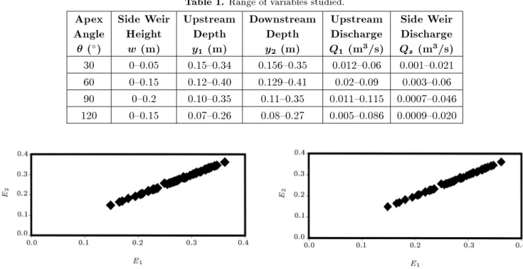
Constancy of Energy

It was assumed by DeMarchi that the specic energy remains constant along the side weir. The present data

(3)

Table 1. Range of variables studied.

Apex

Angle

(

)

Side Weir

Height

w

(m)

Upstream

Depth

y 1

(m)

Downstream

Depth

y 2

(m)

Upstream

Discharge

Q 1

(m

3

/s)

Side Weir

Discharge

Q s

(m

3

/s)

30 0{0.05 0.15{0.34 0.156{0.35 0.012{0.06 0.001{0.021

60 0{0.15 0.12{0.40 0.129{0.41 0.02{0.09 0.003{0.06

90 0{0.2 0.10{0.35 0.11{0.35 0.011{0.115 0.0007{0.046

120 0{0.15 0.07{0.26 0.08{0.27 0.005{0.086 0.0009{0.020

Figure2. Comparison of specic energyE1 andE2for apex angle = 30.

Figure3. Comparison of specic energyE 1 and

E 2for apex angle = 60.

Figure4. Comparison of specic energyE1 andE2for apex angle = 90.

were used in order to check this assumption. Figures 2 to 5 show the comparison of specic energy at the upstream, E

1, and downstream, E

2, of the side weir for dierent apex angles. The average energy dierence between the two ends of a weir, for apex angles of

Figure5. Comparison of specic energyE1 andE2 for apex angle = 120.

30, 60, 90 and 120 degree is 0.59%, 0.55%, 0.72% and 0.94%, respectively. Thus, the assumption of constant energy is accepted for further analysis.

Discharge Coecient

The discharge coecient for a sharp crested, triangular side weir may be inuenced by: 1) The approach velocity of ow \V

1", 2) Upstream depth of ow \ y

00 1, 3) Apex angle \", 4) Width of main channel \B", 5) Width of side channel \B

1" and 6) Height of weir \ w". Dimensional analysis gives:

Cm=f

F 1

B B

1

w y

1

(10)

in which F 1(=

V 1

=(gy 1)

0:5) is the upstream Froude number of the ow. Ramamurthy and Carballada 18] showed the eect ofB=B

1 on the discharge coecient. Borghei et al. 15] indicate that this parameter has a secondary eect onCm. In the present study, B and B

1were kept constant. Therefore, Equation 10 reduces to:

Cm=f

F 1

w y

1

: (11)

Subramanya and Awasthy 4] and Kumar and Pathak 16] reported that the eect ofw=y

1is insignif-icant for sharp crested, rectangular and triangular side weirs, respectively. Borghei et al. 15] and Singh et al. 12] believed that the parameterw=y

1is inuencing Cmfor a rectangular side weir. However, most of the

(4)

investigators have related the discharge coecient,Cm, to approach Froude number,F

1, only.

The values of Cm were calculated using Equa-tion 8 and measured values ofQ

1 y

2 Q

2 b

1 and w, for all the data. Figures 6 to 9 show the variation of discharge coecient,Cm, with the most inuencing parameter, F

1. The following best-t equations were

Figure6. Variation ofCmwithF1 for apex angle = 30 .

obtained for apex angles 30 to 120, respectively: Cm= 0:6458;0:3923F

1 for = 30

(12)

Cm= 0:6108;0:3333F 1 for

= 60

(13)

Cm= 0:637;0:3636F 1 for

= 90

(14)

and:

Cm= 0:5973;0:1834F 1 for

= 120

: (15)

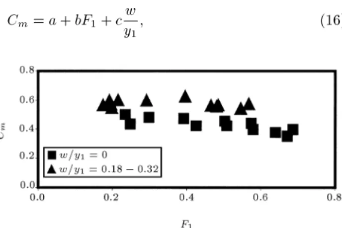
The other inuencing parameter is w=y

1. The typical variation ofCmwithF

1for apex angle 120

is shown in Figure 10. The data used in this gure are those with w=y

1 = 0 and w=y

1 = 0

:18;0:32. This gure shows that for a particular value of apex angle (= 120

) Cm, in addition to F

1 is also, a function of w=y

1. Similar results may be obtained from Figures 11 to 13, which are plots ofCmversusF

1for various values of w=y

1and apex angles 90, 60 and 30, respectively. Therefore, for a particular value of an apex angle, one can write Cm=f(F

1 w=y

1).

To validate the eect of parametersF 1and

w=y 1 and in accordance with the equations proposed by Singh et al. 12] and Jalili and Borghei 19], Cm for a particular value of an apex angle, can be written as the following linear equation:

Cm=a+bF 1+

c w y

1

(16)

Figure 10. Variation ofCmwithF1 andw=y1 for apex angle = 120.

Figure 11. Variation ofCmwithF 1 and

w=y

1 for apex angle = 90.

(5)

Figure12. Variation ofCmwithF1 andw=y1 for apex angle = 60.

Figure13. Variation ofCmwithF1 andw=y1 for apex angle = 30.

where ab and c are constants, which can be found using the experimental data. Using the least square method, the following equations were obtained for various values of an apex angle:

Cm= 0:6246;0:367F 1+ 0

:196 w y

1

for= 30

(17) Cm= 0:5707;0:2932F

1+ 0 :1426

w y

1

for= 60

(18) Cm= 0:5607;0:2511F

1+ 0 :1661

w y

1

for= 90

(19) Cm= 0:5523;0:1317F

1+ 0 :0868

w y

1

for= 120

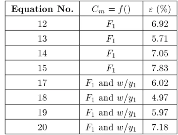
: (20) To have a numerical measure for the best-t line and its ability, in terms of representing the agreement between observed and computed values of a discharge coecient, an average percentage error term, ", was dened as 14,20]:

"= 100 N N X i=1

Cmc;Cmo Cmo (21)

in which N is the number of data and Cmc and Cmo are the computed and observed values of the discharge coecient, respectively. The computed values of "for all the obtained equations for Cm are presented in

Table2. Average percentage error inCmusing dierent equations.

Equation No.

Cm=f() "(%)

12 F 1 6.92 13 F 1 5.71 14 F 1 7.05 15 F 1 7.83 17 F 1and w=y 1 6.02 18 F 1and w=y 1 4.97 19 F 1and w=y 1 5.97 20 F 1and w=y 1 7.18

Table 2. This table shows the comparison of average percentage error, ", obtained when Cm was related to F

1(Equations 12 to 15) and when

Cmwas related toF 1 and wy1 (Equations 17 to 20). It is obvious that using Equations 17 to 20 improves the average percentage error. Because use of these equations generally leads to lower values of"(Table 2), Equations 17 to 20 are preferred and can be taken as a discharge coecient in the DeMarchi equation for subcritical ow.

Equations 4, 8 and 17 to 20 aord a means of calculating the discharge over sharp crested triangular side weirs of apex angles 30 to 120, respectively.

APPLICATION

Design Procedure

The design of the side weir to pass a certain discharge, Qs, into the side channel, involves the determination of the side channel width, B

1, and weir height, w, for given values of the upstream discharge,Q

1. For design discharge,B

1is kept equal to b

1. The steps for design are as follows:

1. For a side weir with known apex angle, assume a suitable value forw

2. CalculateQ 2, using

Q 2=

Q 1

;Qs 3. Calculate normal depth of ow, y

2, and, hence, specic energy,E

2, by: E 2= y 2+ Q 2 2 2gB 2 y 2 2 (22)

4. By assuming that specic energy remains constant along the length of the side weir, i.e.,E

1= E

2= E, determiney

1using the following equation: E 1= y 1+ Q 2 1 2gB 2 y 2 1 (23)

5. CalculateF

1and, hence,

Cmfrom Equations 17 to 20, as the case may be

(6)

6. Determine value ofb

1from Equation 8. If this value is much dierent from the width of the proposed side channel,B

1, suitable changes may be made in wand the procedure is repeated untilb

1 =B

1.

Discharge Calculation

Computation of the discharge over a given side weir (with known values of andw) into a side channel of known widthB

1, is possible for given values of y

1 and Q

1. The steps to be followed are as follows:

1. For the depth of ow and discharge in the upstream section,y

1and Q

1, calculate E

1using Equation 23 2. Determine value ofF

1 and, hence,

Cm from Equa-tions 17-20, as the case may be

3. By assuming that E 1 =

E 2 =

E, calculate y 2, using Equation 8, forb

1= B

1(maximum side weir discharge) or measured value ofb

1 4. Calculate downstream discharge, Q

2, from Equa-tion 4

5. Determine side weir discharge,Qs, from Equation 9.

CONCLUSION

It was shown that the DeMarchi equation can be used to estimate the discharge over a sharp crested, triangular side weir. It was observed that the specic energy remains constant along the triangular side weir. The DeMarchi coecient of discharge for a sharp crested triangular side weir in subcritical ow is a function of the approach Froude number in the main channel, the apex angle of the weir and ratio of weir height to upstream depth of ow. New equations for the discharge coecient were introduced, which enable determination of side weir discharge. The procedures for design and computation of discharge for a triangular side weir were also introduced.

NOMENCLATURE

A cross sectional area of ow

B width of main channel

B

1 width of side channel

b

1 distance between sections 1 and 2 along the weir

Cm DeMarchi coecient of discharge

E specic energy

F

1 approach Froude number

g acceleration due to gravity

Q discharge in the channel

Qs discharge over side weir

Sf friction slope

S

0 slope of channel bed

T top width of channel section V average velocity in main channel

w weir height

x distance along side weir

y depth of ow

kinetic energy correction factor " average percentage error

apex angle

DeMarchi varied ow function

suxes 1 and 2 denotes the upstream and downstream conditions, respectively

REFERENCES

1. Allen, Y.W. \The discharge of water over side weirs in circular pipes", Proceedings, Institution of Civil Engineering, London,6, pp 270-287 (1957).

2. Colling, V.K. \The discharge capacity of side weirs",

Proceedings, Institution of Civil Engineering, London, 6, pp 288-304 (1957).

3. Frazer, W. \The behavior of side weirs in prismatic rectangular channels",Proceeding, Institution of Civil Engineering, London,6, pp 305-328 (1957).

4. Subramanya, K. and Awasthy, S.C. \Spatially varied ow over side weirs", J. Hydr. Engrg., ASCE, 98(1), pp 1-10 (1972).

5. Smith, K.V.H. \Computer programming for ow over side weir", J. Hydr. Engrg., ASCE, 98(1), pp 1-10 (1973).

6. El-Khashab, A. and Smith, K.V.H. \Experimental investigation of ow over side weirs",J. Hydr. Engrg., ASCE,102(9), pp 1255-1268 (1976).

7. Ranga Raju, K.G., Prasad, B. and Gupta, S. \Side weirs in rectangular channels",J. Hydr. Engrg., ASCE, 105(5), pp 547-554 (1979).

8. Hager, W.H. \Hydraulics of distribution channel",

Proc. 20th Congress, IAHR, Moscow, pp 534-541 (1983).

9. Hager, W.H. \Lateral out ow over side weirs", J. Hydr. Engrg., ASCE,113(4), pp 491-503 (1987). 10. Uyumaz, A. and Smith, R.H. \Design procedure for

ow over side weirs", J. Irrig. and Drain. Engrg., ASCE,117(1), pp 79-90 (1991).

11. Uyumaz, A. \Side weir in triangular channel",J. Irrig. and Drain. Engrg., ASCE,118(6), pp 965-970 (1992). 12. Singh, R., Manivannana, D. and Satyanarayana, T. \Discharge coecient of rectangular side weir", J. Irrig. and Drain. Engrg., ASCE,120(4), pp 814-819 (1994).

13. Swamee, P.K., Pathak, S.K. and Sabzeh Ali, M. \Side weir using elementary discharge coecient", J. Irrig. and Drain. Engrg., ASCE,120(4), pp 742-755 (1994).

(7)

14. Ghodsian, M. \Elementary discharge coecient for rectangular side weir",Proceeding of 4th International Conference on Civil Engineering,IV, pp 36-42 (1997). 15. Borghei, S.M., Jallili and Ghodsian, M., \Discharge coecient for sharp crested side weir in subcritical ow",J. Hydr. Engrg., ASCE,125(10), pp 1051-1056 (1999).

16. Kumar, C.P. and Pathak, S.K. \Triangular side weirs",

J. Irrig. and Drain. Engrg., ASCE,113(1), pp 98-105 (1987).

17. Henderson, F.M., Open Channel Flow, Macmillan,

New York, N.Y., USA (1966).

18. Ramamurthy, A.S. and Carballada, L. \Lateral weir ow model", J. Irrig. and Drain. Engrg., ASCE, 106(1), pp 9-25 (1980).

19. Jalili, M.R. and Borghei, S.M. \Discussion of discharge coecient of rectangular side weir", J. Irrig. and Drain. Engrg., ASCE,122(1), pp 132 (1996).

20. Ghodsian, M. \Viscosity and surface tension eects on rectangular weir ow",Int. Journal of Engineering Science,9(4), pp 111-117 (1998).