Sharif University of Technology
Scientia IranicaTransactions B: Mechanical Engineering www.scientiairanica.com
Evaluation of the modied 3D free-surface Green's
function for potential ow in a numerical towing tank
A. Abbasnia and M. Ghiasi
Department of Marine Engineering, Amirkabir University of Technology, Tehran, Iran. Received 31 May 2012; received in revised form 23 December 2012; accepted 25 June 2013
KEYWORDS The source; Boundary-value problems; Numerical towing tank;
Green's function; Image method.
Abstract.What is derived in this paper is the potential ow around the marine structures in the numerical towing tank. The Green's formula and image method is employed to solve the boundary value problem. The Green's function satises the Laplace equation and the boundary conditions on the bottom, walls and free surface. The Green's function consists of three parts. The rst part is correlated with spatial spacing between the source and a eld point. The second part consists of the free surface disturbance. The radiation condition is dealt with in the third part to ensure that the waves vanish upstream of the source. An innite series is obtained for each part of the Green's function using the image method. Eects of the numerical towing tank's width and depth on the solution are investigated, and the ow patterns due to the presence of a singularity with constant strength in the uniform ow are computed. Uniform motion of a submerged sphere and ellipsoid are simulated and compared with the analytical solutions and other numerical results. Wave proles are computed for a sphere and an ellipsoid to show the eect of the tank width on the solution. © 2013 Sharif University of Technology. All rights reserved.
1. Introduction
Hydrodynamic analysis of the marine structures in the towing tanks is necessary for obtaining the perfect design in ocean engineering. The towing tanks have been widely used for various marine purposes one of which is to determine the performance of the marine structures in a uniform motion and the properties of ow around the body of the structure. Motions of structures in a harbor and the model test in the towing tank could be aected by side walls and the bottom (sea bed). Development of the Numerical Towing Tank (NTT) can help to account for the nite boundary eects induced by the walls and bottoms of the physical tanks and to make the test results more precise, which would eventually reduce the test cost.
*. Corresponding author. Tel.: +98-21-66419615 E-mail addresses: a [email protected] (A. Abbasnia), [email protected] (M. Ghiasi)
The potential theory in computational hydrody-namics is widely used to characterize the interactions of uid-marine structures. The governing equation in incompressible, inviscid uid and irrotational ow is Laplace's equation whose solutions must satisfy the various boundary conditions. NTT boundary condi-tions consist of the free-surface boundary condition, the impermeable boundary conditions of the body, wall sides and the bottom, the inow boundary condition and the radiation boundary condition of the outow surface, to ensure that the waves vanish upstream of the disturbance. The Boundary Elements Method (BEM), based on the second Green's identity, has been employed to solve the boundary value problems with complex geometry of boundaries. The fundamental Green's function for a towing tank can be assumed to be the Green's function of a source with constant strength on the NTT where the boundary conditions are the conditions on the bottom, walls and the free surface. The fundamental Green's function can be used
with the body boundary condition for simulation of the ow on the NTT with presence of the body. Other boundary conditions are satised spontaneously.
Various Green's functions were presented in com-plex and algebraic formulations for two and three dimensional problems by Wehausen & Laitone [1]. The Green's function is approximated by solving the place-Laplace equation in dierent computational domains and specied boundary conditions. The approxima-tion algorithm of the fundamental soluapproxima-tion has been based on Fourier transforms space and inverse Fourier transforms given by Newman [2]. Evaluation of a Principal Value (PV) integral would be unavoidable in a computational application. The singularity in a PV integral could be removed by Cauchy's residue theorem. The shallow water Green's function of uniform ow was modied by Sahin and Hyman [3] and was used in the ow simulation of the uniform motion of a submerged body presented by Sahin et al. [4]. The source in parallel planes and rectangular channels was developed by the image method, a restricted domain Green's function can be obtained by distribution of sources along the length of a normal line to the planes and by formal summation of the Green's functions in the computational domain. Innite series arising from the application of image methods are slowly conver-gent [2,4,5]. Dierent remedies have been introduced to change these series of images into rapidly convergent formulations. The Green's function of a channel water-wave with innite depth was obtained by Kashiwagi [6] in which slowly convergent series were transformed by a double integral over a semi-innite domain. The 3D acoustic Green's function in a rectangular channel was given by Newman [7] in which sources in two transverse directions were distributed, and Fourier techniques were applied to transform an innite series of images into an applied Green's function. Oscillating source problems in channels with innite and nite depth were solved by Linton [5]. For innite and nite depth, the slowly convergent series were rewritten into a rapidly convergent series by Eigen function expansion. For nite depth channels, orthonormal sets of functions are also adopted. A suitable Green's function is proposed by Xia [8] for 3D wave-body interaction problems in the channels. This formulation is based on the open-sea Green's function. The innite series of images are evaluated through the asymptotic analysis. Solutions of a 3D acoustic source in parallel planes and an innite open rectangular prism were expressed as a series of images by Ismail and Elbenhady [9]. They used the Eigen function expansions to transform slowly convergent series into an integral representation, which is rapidly convergent and stable.
Numerical tanks have been developed since the past two decades to compute ow eld around objects in presence of the free surface. Potential numerical
tank has been based on boundary integral equation and MEL (Mixed Eulerian-Lagrangian) method. Free surface is included in boundary integral explicitly, and its mutations have been obtained through transforming free surface boundary condition from Eulerian form into Lagrangian form. A 2D wave-current interaction was investigated by Ryu et al. [10], and 3D wave-current interaction modeling was carried out by Zhen and Bin [11]. In these numerical tanks, 2D and 3D acoustic Green's function are distributed over the free surface and inow and outow boundaries to satisfy the radiation condition in the integral equation. So, com-putations are time-consuming with numerical errors. Also, the description of the free surface uctuation is complicated.
Dawson method has been applied in direct and indirect BIE (Boundary Integral Equation) to study the eect of free surface on uid ow around moving, oating and submerged bodies. The performance of moving 3D hydrofoil was examined by Xie and Vas-salas [12]. Applying free surface boundary condition to BIE is a little tricky and too sensitive to the size and shape of the free surface grids. Therefore, this scheme is not reliable for practical approaches.
An ecient and accurate technique was proposed by Scullen and Tuck [13] to compute a 3D fundamental solution of uniformly and non-uniformly distribution of moving pressure patches for far eld and near eld domain. The multiple expansions were applied to the 3D free surface Green's function of oscillation source by Borgarino et al. [14]. It is pointed out that the recently mentioned Green's functions have been practiced in open-sea condition. Hence, the achievement of a practical 3D free surface Green's function of restricted condition for an NTT could be useful.
In the present work, Green's function of a source with constant strength in a uniform ow is evaluated for a rectangular tank with arbitrary dimensions. The boundary conditions contain linearized free-surface conditions, impermeable boundary conditions on the bottom and side walls, and the radiation condition. Open-sea nite-depth Green's function will be adopted in the evaluation procedure. The proposed Green's function includes the mentioned boundary conditions, except the side walls boundary condition. Numerical towing tank Green's function would be approximated by distribution of images of the source on the length of normal direction of the wall and formal summation of the Green's functions on the computational domain. The Green's function of a practical numerical towing tank is aimed in this study. For this purpose, this innite series will be discrete in three parts. The rst part includes the slowly convergent series of the 1=r term. In the second and third parts, the inte-grals of innite series are approximated. The rapidly convergent form of the rst part can be obtained
based on Eigen function expansions. Cauchy's integral theorem and Poisson's summation formula combined with a convergent geometric series are employed to compute the principle value integrals in the series of the second part. In the same manner, the denite integral in the series of the third term is evaluated. The dependency of the ow properties to width and depth of the tank are shown and veried by the modied open-sea free-surface Green's function. Modeling of a uniform motion of a submerged sphere and ellipsoid in a numerical towing tank are developed on the basis of the constant panel method. Simulation of uid ow around a sphere is compared with analytical solutions and other numerical results. Center plane wave proles of a sphere and an ellipsoid are obtained to study the eects of tank width on the solution for various tank dimensions and dierent ow regimes.
2. Background
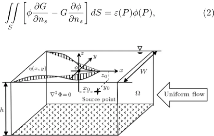
The Cartesian coordinates system is chosen with the (x; y) plane on the undisturbed free surface, and z is measured vertically upwards. The width of the tank is W and its depth is h as shown in Figure 1. Fluid is assumed to be inviscid and incompressible, and the ow is irrotational. Therefore, the Laplace equation is the governing equation in the computational domain ().
Fluid ow around a body that moves uniformly in the towing tank in +x direction could be computed by potential theory. Hence, velocity potential () is composed of the uniform ow velocity potential in x direction, and perturbation velocity potential induced by the existence of the body.
(x; y; z) = | {z }U:x
Uniform ow potential
+ (x; y; z)| {z }
Perturbation potential
: (1) To compute the perturbation potential, the panel method based on Green's second identity is applied. The direct boundary integral equation for perturbation potential can be written as:
ZZ
S
@n@G
s G
@ @ns
dS = "(P )(P ); (2)
Figure 1. Cartesian system and tank geometry.
where P is a eld point positioned on the body surface, walls, bottom or in the uid domain; S is the control surface of a numerical towing tank, and ~n is the normal vector on a control surface directed into the uid. The value of " depends on the location of the eld point. Green's function (G) is the solution of Eq. (3) that must satisfy the boundary conditions.
r2G = (x x
0)(y y0)(z z0) in ; (3)
where is the Dirac delta function. Indeed, a constant strength source in uniform ow at (x0; y0; z0) disturbs
the whole uid ow domain (x; y; z). Green's function represents the source disturbance aected by a set of boundary conditions. NTT boundary conditions contain the following.
Free surface boundary condition: Free surface elevation (x; y) is measured from the calm water level. This boundary condition is made of a combination of dynamic and kinematics boundary conditions.
@2G
@x2 + K0
@G
@z = 0; on z = 0; (4) where K0= g=U2.
Bottom condition: The tank bottom is imperme-able and its slope is zero; therefore, the normal derivative of the Green's function must be considered as to be zero:
@G
@z = 0 on z = h: (5) Radiation condition: To ensure that the distur-bance wave would shrink upstream and to obtain a unique solution for the boundary value problem, the radiation condition is applied:
lim G
r2!1= O(1); for x < 0;
lim G
r2!1= 0; for x > 0; (6)
where:
r =p(x x0)2+ (y y0)2+ (z z0)2:
Tank's wall condition: The normal derivative of the fundamental solution must be zero, owing to the impermeable walls of the tank:
@G
@y = 0 on y = W
2 : (7)
If the solution of Eq. (3) satises the NTT boundary conditions, the control surface in Eq. (2) is limited to the body surface.
3. Formulation of Green's function
The open-sea Green's function in the nite depth for a constant strength source located at (0; 0; z0) given by
Wehausen and Laitone [1] can be rewritten as:
Go= I1+4I2+ 4I3: (8)
The term I1 represents the source and its image with
respect to the bottom. The term I2 indicates the free
surface disturbance due to the presence of the source, and its image and the term I3 exists to satisfy the
radiation condition [15]. For K0h > 1,
I1= r1 1+
1
r2; (9)
where: r2
1= x2+ y2+ (z z0)2;
r2
2= x2+ y2+ (z + (2h + z0))2;
and:
I2= P V 1
Z
0 =2
Z
0
F (; k; z) cos(kx cos )
cos(ky sin )ddk; (10) where:
F (; k; z) =ecosh(kh)(k Kkhcosh[k(h + z0)](k + K0sec2)
0sec2 tanh(kh))
cosh(k(h + z)); and:
I3= =2
Z
0
H(; K; z) sin(Kx cos ) cos(Ky sin )d; (11) where:
H(; K; z) =ecosh(Kh)(1 KKhcosh[K(h + z0)](K + K0sec2)
0sec2 sec h2(Kh))
cosh(K(z + h)):
In function F , k is integration variable and in function H, K is the wave number which can be determined by Eq. (12):
K K0sec2 tanh(Kh) = 0: (12)
3.1. Image method
To use the image method, the walls of the tank are removed, and the control volume becomes unbounded in the transverse direction. Instead, an innite series of the images of the source are distributed over the normal axis to the walls of the tank, as shown in Figure 2. According to Figure 2, the position of the images in the y direction in an unbounded domain can be written as:
y0
0= y0+ 2nW; n = 1 1;
y00
0 = y0+ (2n + 1)W; n = 1 1: (13)
Green's function for the image of each source can be approximated by substituting its position in Eq. (8). Then, the Green's function of the tank can be expressed by formal summation of these innite Green's functions as:
G =
1
X
n= 1
(I0 1+ I100)
| {z }
J1
+4
1
X
n= 1
(I0 2+ I200)
| {z }
J2
+ 4
1
X
n= 1
(I0 3+ I300)
| {z }
J3
; (14)
where J1represents source and its images with respect
to the walls of the tank and the bottom of the tank.
J1= 1
X
n= 1
1 r0
1+
1 r00
1 +
1 r0
2+
1 r00
2
; (15)
in which: r02
1 = (x x0)2+ (y y00)2+ (z z0)2;
r002
1 = (x x0)2+ (y y000)2+ (z z0)2;
r02
2 = (x x0)2+ (y y00)2+ (z + (2h + z0))2;
r002
2 = (x x0)2+ (y y000)2+ (z + (2h + z0))2:
Figure 2. Image method scheme with respect to the tank walls.
The second and third term (J2, J3) could be re-written
in complex space as follows:
J2= Re
( 1 X
n= 1
P V
1
Z
0
dk
=2
Z
0
F (; k; z) cos[k(x x0) cos ]
heik(y y0+2nW ) sin +eik(y+y0+W +2nW ) sin id
)
= Re (
P V
1
Z
0
dk
1
X
n= 1 =2
Z
0
[F1(; k; x; y; z)
+ F2(; k; x; y; z)] eik2nW sin d
) ;
(16) in which:
F1(; k; x; y; z)
= F (; k; z) cos[k(x x0) cos ]eik[y y0] sin ;
F2(; k; x; y; z)
= F (; k; z) cos[k(x x0) cos ]eik[y+y0+W ] sin ;
and:
J3= Re
( 1 X
n= 1 =2
Z
0
G(; K; z) sin[K(x x0) cos ]
heiK(y y0+2nW ) sin +eiK(y+y0+W +2nW ) sin id
)
= Re ( 1
X
n= 1 =2
Z
0
[G1(; K; x; y; z)
+ G2(; K; x; y; z)] eiK2nW sin d
) ;
(17) where:
G1(; K; x; y; z)
= G(; K; z) sin[K(x x0) cos ]eiK[y y0] sin ;
G2(; K; x; y; z)
=G(; K; z) sin[K(x x0) cos ]eiK[y+y0+W ] sin :
3.2. Asymptotic analysis for J1
Slow convergence of the series in Eq. (15) causes diculties in numerical applications [2,16]. The Eigen function expansions and their deriving approaches given by Ismail and Elbenhady [9] are adopted to obtain an applicable form of J1. For a singularity 1=r
in the middle of parallel planes, the Green's function ( G) is written as [16]:
G(; y; ) = (2+ y2) 1=2
+ X1
m= 1 m6=0
n
2+ (y m)2 1=2 jmj 1o; (18)
where is the width of parallel planes, and = p
x2+ z2. In the innite series in Eq. (18),
jmj 1parameter, as a constant, is subtracted from
each term of fundamental solution to reach to the con-vergent series. Using the Eigen function expansions can make the Green's function be more rapidly convergent. An alternative form of Eq. (18) is given as [16]:
G(; y)= 2C+ln2+4
1
X
m=1
k0(2m) cos(2my);
(19) where C = 0:577215665 is the Euler's constant given by Gradshteyn and Ryzhik [15], and k0is the modied
Bessel function of the second kind of order zero. In Eq. (15), the four slow convergent innite series of singularities can be written for 2W .
S1= (x x0)2+ (y y0)2+ (z z0)2 1=2
+ +1X
n= 1
n6=0
n
(x x0)2+ (z z0)2
+ (y y0 2nW )2 1=2 j2nW j 1
o
; (20)
S2= (x x0)2+ (y y0 W )2+ (z z0)2 1=2
+
+1
X
n= 1
n6=0
n
(x x0)2+ (z z0)2
+ (y + y0 W 2nW )2 1=2 j2nW j 1
o ; (21)
S3= (x x0)2+ (y y0)2+ (z + (2h + z0))2 1=2
+
+1
X
n= 1
n6=0
n
(x x0)2+ (z + (2h + z0))2
+ (y y0 2nW )2 1=2 j2nW j 1
o
S4= (x x0)2+(y+y0 W )2+(z+(2h+z0))2 1=2
+ +1X
n= 1
n6=0
n
(x x0)2+ (z + (2h + z0))2
+ (y + y0 W 2nW )2 1=2 j2nW j 1
o : (23) By substituting Eqs. (20)-(23) into Eq. (19), four rapidly convergent series are obtained. For example, S1 series can be written in the following form:
S1= 2 C + ln
p
(x x0)2+ (z z0)2
2
!
+ 4X1
m=1
B0
2mp(x x0)2+ (z z0)2
cos [2m(y y0)] : (24)
Other series can be transformed in the same manner. Formal summation of convergent series S1, S2, S3,
S4 makes a unique series for application in numerical
computation.
3.3. Modifying analysis for J2 and J3
Simplication of J2 and J3 from the integral series
to a simpler form can be carried out by the Poisson summation formula described in general form as:
SN= 1 X n= 1 b Z a
E()einf()d = b Z a E() 1 X n= 1
e2f()d;
(25) where E() is an arbitrary function. Using a convergent geometric series given by Gradshteyn and Ryzhik [15], we have:
N 1X n= N
en= eN e N
e 1 ; (26)
and substituting Eq. (26) into Eq. (25), we have:
SN = b
Z
a
F ()
eiNf() e iNf()
eif() 1 d;
when N ! 1; (27)
where F () is an arbitrary function and the integrand has poles on m = 2m. Taylor expansion of f
function for = m+ p can be written as:
f() = f(m) + pf0(m) + p2=2f00(m) +
2m + pf0(
m): (28)
Thus:
eif() 1 = eipf0(
m) ipf0(
m); as p ! 0:
(29) There might be a number of such poles at [a; b] in Eq. (27) when N ! 1. If each pole has the vicinity ( "; "), then Eq. (27) can be obtained as:
SN =
X
m "
Z
"
F (m)
h eiNpf0(
m) e iNpf0(m)
i
ipf0(m) dp:
(30) By substituting:
u = Npf0( m);
du = Nf0( m)dp;
R = N"f0( m):
Eq. (31) can be achieved.
SN = 0
X
m
F (m) if0(m)
R
Z
R
[eiu e iu]
u du
+ f0( m) > 0
f0(
m) < 0 = 0
X
m
2F (m)
jf0(m)j; (31)
where P0 denotes that if = a or = b, the term m = 0 must be halved. In the same manner, Eqs. (16) and (17) can be modied for (0 =2), and the modied form of the equations can be written as:
J2=Re
( P V 1 Z 0 dkW 1 X m=0 0
F (m; k; z)
k cos m
cos(kx cos m)eiky sin m
e iky0sin m+ ( 1)meiky0sin m
)
=2WP V
1
Z
0
dkW X1
m=0 0
F (m; k; z)
k cos m
cos(kx cos m)
(
cos(ky sin m) cos(ky0sin m)
in which cos and sin depend on the odd and even value of m, respectively, and k sin m= m=W .
J3=2W 1
X
m=0 0
e Kmh(K0+ Kmcos2m)
1 K0h sec h2(Kmh) + sin2m
cosh(Km(z + h))
cosh(Kmh) cosh(Km(z0+ h))
sin(KmK(x x0) cos m)
mcos m
(
cos(Kmy sin m) cos(Kmy0sin m)
sin(Kmy sin m) sin(Kmy0sin m) (33)
Also, cos and sin depend on the odd and even value of m, respectively, and Kmsin m= m=W .
3.4. Evaluation of the principal value integral in J2
In general, Cauchy principal value integral could be introduced for the rst order pole as follows:
I = lim
jxj!1 b
Z
a
D(k)
k Keid(k)xdk = iD(K)eid(K)x(34);
in which the sign is for x < 0 and the + sign is for x > 0. Function g is dened as follows:
g(k) = k K0sec2mtanh(kh) = 0: (35)
Using a derivative of function g with respect to k and k sin m = m=W , the Taylor expansion of this
function can be written as: g(k)=g0(K)(k K)=(1 K
0h sec2msec h2(Kh)
+ 2K0tan2msec2mtanh(Kh)=K)(k K)
= sec2
m(1 K0h sec h2(Kh)+sin2m)(k K):
(36) It can be shown that K = Kmfor Kmsin m= m=W .
If function D and function d are dened as:
D(Km) = e
Kmhcosh[Km(h + z0)]
(1 K0h sec h2(Kmh) + sin2m)
(K0+ Kmcos2)cos[Kcosh(Km(z + h)] mH)
K 1
mcos m
(
cos(ky sin m) cos(ky0sin m)
sin(ky sin m) sin(ky0sin m) (37)
d(Km) = Kmcos m; (38)
then the principal value integral, J2, can be calculated
as:
J2=2W 1
X
m=0 0
fReal(I)g
=2W
1
X
m=0 0
fD(Km) sin(Km(x x0) cos m)g
= 22 W
1
X
m=0 0
e Kmh(K0+ Kmcos2m)
(1 K0h sec h2(Kmh) + sin2m)
cosh(Kcosh(Km(z0+ h))
mh) cosh(Km(z + h))
sin(KmK(x x0) cos m)
mcos m
(
cos(Kmy sin m) cos(Kmy0sin m)
sin(Kmy sin m) sin(Kmy0sin m) (39)
4. Analysis of results
The ecient free-surface Green's function in a nu-merical towing tank is developed in this paper. The open-sea Green's function and image method are em-ployed to obtain an appropriate NTT Green's function. Asymptotic analysis based on Eigen function expan-sions and the Cauchy principal value integral associated with the Poisson summation formula are applied to re-move computational singularities (i.e. slow convergent innite series in the principal value integral).
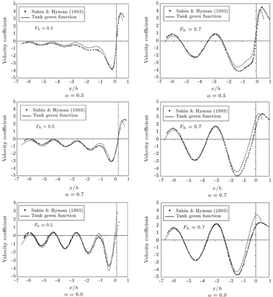
Usually, the physical towing tank is used to test models in open-sea and restricted water conditions. Therefore, the NTT Green's function must be tested and be able to model the open-sea and restricted water conditions. In the following, numerical computation of NTT Green's function is carried out for two case studies, i.e. uniform motion of a submerged sphere and an ellipsoid. Added mass and the distribution of potential over the body sphere in open-sea conditions are calculated and compared with the analytic and numerical solutions. The eect of the wall of the tank on the free-surface disturbance induced by a sphere and an ellipsoid motion in the tank is also investigated. 4.1. Towing tank Green's function verication The towing tanks have been widely used to determine uid ow and hydrodynamic resistance for the bodies moving in the open-sea and restricted water conditions. Figure 3 shows the results of the proposed towing tank Green's function and the open-sea Green's function of a singularity located at (0; 0; f) in the uniform ow proposed by Sahin and Hyman [3]. The submergence depth parameter of a source point is dened by =
Figure 3. Comparison of velocity coecient of a source in the open-sea condition.
(h f)=h, and the depth Froude number is dened as Fh= U=pgh. Velocity coecient is = (@G=@x)h2=m
in which m is the source strength computed at (y = 0; z = h). Velocity coecient is calculated in two ow regimes (Fh= 0:5, 0:7) and dierent submergence
depth parameters of the sources. It is worth mentioning that the width of the towing tank is taken very large (1000h) for the comparison of the results obtained by the modied Green's function and the results reported by Sahin and Hyman [3].
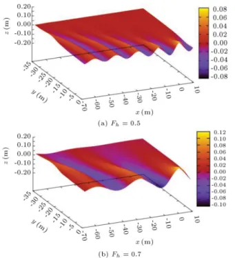
The disturbance wave pattern can be approx-imated through the linearized dynamic free-surface boundary condition as below:
= U@G@x: (40) Wave propagation in open-sea state induced by the existence of a source point in uniform ow is illus-trated over half of the domain in Figure 4 for two
dierent ow regimes (dierent depth Froude number) and a constant submergence depth parameter. It is shown that a wave pattern for a constant submergence depth parameter is severely aected by ow regimes. The amplitude of wave is increased, and waves are propagating divergently as the uniform ow velocity is increased. The wave pattern for a source point with a constant depth Froude number (Fh) and dierent depth
parameter () is illustrated in Figure 5. It shows that when submergence depth parameter is increased, the disturbance wave amplitude enlarges and wave pattern diverges.
Reected waves from the walls of the tank are essential for the investigation of the eect of walls on the free-surface disturbance and capability of the image method to model the tank walls boundary condition. Figure 6 shows the wave pattern of a source point located at a constant depth parameter under the dierent ow regimes in a towing tank. Meanwhile,
Figure 4. Disturbance wave pattern of a source in the dierent ow regimes (depth Froude number) at = 0:5.
Figure 5. Wave pattern comparison of a source in a constant ow regime (Fh= 0:7) and various ; SL ( = 0:7), SR ( = 0:9).
when the wave pattern is more divergent, the fully developed reected wave eld is beginning farther than the source point.
4.2. Numerical examples
The modied towing tank Green's function is applied in a numerical computation of the motion of a sphere and an ellipsoid in NTT. The distribution of the velocity potential over a sphere and the surge added mass (m11) are computed and compared with the analytical
solutions and the existing numerical results. In this study, the direct boundary integral method is used to compute potential uid ow. The body surface is described by triangle panels as shown in Figure 7.
The towing tank Green's function is substituted in
Figure 6. Wave pattern of a source in the NTT with a constant submergence depth parameter ( = 0:7) and the tank's width 30 (m) at various ow regimes.
Figure 7. Triangle meshes over the body surface.
the Green's formula for modeling the uniform motion of a oating or submerged body in the numerical towing tank. The second Green's identity is written as:
ZZ
Sq
q@G@nPq
q GPq
@ @nq
dSq = "(P )(P ); (41)
where P is a eld point, q is a source point, and Sq
indicates body surface. "(P ) depends on the position of the eld point, which can be located on the body surface ("(P ) = 2) or in the control volume ("(P ) = 4) or out of the domain ("(P ) = 0). The constant
panel method is used in the numerical computation. The distribution of velocity potential over the panels is assumed to be constant, and the source point is located at the center of each panel. On each panel, the normal ux of potential (body boundary condition) is the known value, and the potential is the unknown value that must be calculated. Impermeable body condition is expressed as:
@ @n
Sq
= 0 ! @@n
Sq
= Unx; (42)
in which nxis x coordinate of body unit normal vector
directed into the uid. The descritized form of Eq. (41) can be written as:
N
X
j=1
2 6 4j
ZZ
Sj
@Gij
@njdSj+2jij
3 7 5=
N
X
j=1
ZZ
Sj
GijU~i:~njdSj;
(43)
where is Kronecker delta function, and j indicates the number of panels and i shows the eld point. Eq. (43) is an algebraic system of equations with unknown values on the left hand side and the vector of known values on the right side of equation.
The uniform motion of a sphere with radius r and U = 1m=s in an unbounded uid is simulated. Determination of perturbation potential on the sphere body is veried by computation of the surge added mass (m11) and distribution potential over the body
surface. The added masses are dened as:
mij = ;
ZZ
Sq
j@@njdS; i; j = 1; 2; 6: (44)
Table 1 shows the result of computation of the surge added mass, using the proposed Green's function and the exact solution. It is shown that accurate results can be obtained by present Green's function. However, increase in the number of panels results in decrease in the error of computation.
The distribution of velocity potential over the sphere is calculated in unrestricted water to prove the simulation in this numerical towing tank. The radius of
the sphere is taken to be 1 and the unbounded uniform ow is from x direction with its speed U = 1m=s. The perturbation potential along the polar angle, = 0 deg. to = 90 deg., at the y plane on sphere surface are computed and compared with the exact solution and Kim and Shin calculations [17] in Figure 8. To compare the results with Kim and Shin [17], the computation is conducted for the tank with very large dimensions (h = 100f, W = 1000h).
Furthermore, the eect of tank width on the surge added mass coecient (m11=r3) of this unit radius
sphere is shown in Figure 9. It was shown that surge added mass was increased severely as tanks width was decreased for a constant depth. The walls of the tank restrict uid ow around the body and uid particles are forced to pass the body more quickly by decreasing the tank width.
Figure 8. Perturbation potential on the sphere surface.
Figure 9. Surge added mass coecient of the unite radius sphere in the towing tank (Fh= 0:1) with various width. Table 1. The surge added mass of a sphere.
No. of panels NTT solution of m11=r3
Exact solution of
m11=r3 % of error Abs. error 512 6.7605E-01 6.6667E-01 1.4075E+00 9.3833E-03 768 6.7592E-01 6.6667E-01 1.3880E+00 9.2533E-03 1064 6.6754E-01 6.6667E-01 1.3100E-01 8.7333E-04 1565 6.6700E-01 6.6667E-01 5.0000E-02 3.3333E-04 2048 6.6698E-01 6.6667E-01 4.6499 E-02 3.1000E-04 3072 6.6701E-01 6.6667E-01 5.0999E-02 3.4000E-04
Furthermore, Figure 10 presents a comparison of the dimensionless wave elevation (=h) of the center plane in an unbounded domain for the various tanks width -to- bodies width W=B in a constant submerged depth parameter and a constant ow regime. Longitu-dinal length of ellipsoid is 2b and transverse length in z direction is 2a and in y direction is 2c.
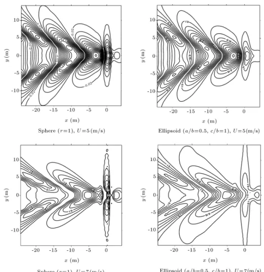
Contours of wave patterns due to the presence of a
sphere and ellipsoid in open-sea conditions with various ow velocities are presented in Figure 11. Submergence depths of bodies are 2(m) under the free-surface.
5. Conclusion
The measuring of hydrodynamic characteristics, re-sistance and analysis of uid ow for a body
mov-Figure 10. Comparison of calculated center plane wave prole in unbounded and at various W=B for a sphere and an ellipsoid at Fh= 0:7 and = 0:5.
ing uniformly in open-sea conditions or in restricted water conditions are usually carried out by towing tank experiments which could be expensive and time-consuming. Numerical computation is a powerful tool for simulating the motions of a body in NTT. How-ever, accuracy of the results depends on the method and the Green's function used in the computation. Green's function is a fundamental solution of Laplace equation for a constant strength source, which satises specic boundary conditions. Free-surface boundary conditions, impermeable bottom and walls of the tank condition, and the radiation condition on upstream of the source are considered in the fundamental solution of towing tank. A modied Green's function for numerical towing tank is developed on the basis of the free surface Green's function for unbounded domain. The NTT Green's function contains innite slow convergent series and principal value integrals whose numerical application causes diculties in the solutions. The Eigen function expansions and the Poisson summation formula combined with the Cauchy principal value integral are employed to overcome the diculties of numerical computation.
Tank walls conne streamline ow around the body, and cause the uid to travel the body surface more rapidly than in the absence of the tank walls. The ow regime and the width of the tank aect the ow characteristics around the body in the towing tank, and consequently change the free surface disturbance. It could be shown that the wave amplitude was increased when the width of the tank was decreased. Indeed, wa-ter accumulation due to the wall and bottom boundary results in the change in the ow streamlines and the increase in water particle velocity and wave making resistance.
References
1. Wehausen, J.V. and Laitone, E.V., Surface Waves, Springer-Verlag, New York (1960).
2. Newman, J.N. \Algorithms for the free-surface Green function", J. Eng. Math., 19, pp. 57-67 (1985).
3. Sahin, I. and Hyman, M. \Numerical calculation for the ow of submerged bodies under a free curface", Ocean Eng., 20(3), pp. 339-347 (1993).
4. Sahin, I., Hyman, M. and Nguyen, T.C. \Three dimensional ow around a submerged body in nite-depth water", J. Appl. Math. Model, 18, pp. 611-619 (1994).
5. Linton, C.M. \On the free-surface Green's function for channel problems", Appl. Ocean Res., 15(5), pp. 263-267 (1993).
6. Kashiwagi, M. \Radiation and diraction forces acting on a three-dimensional body in a narrow tank", Int. J. Oshore Polar Eng., 1, pp. 101-107 (1991).
7. Newman, J.N. \The Green function for potential ow
in rectangular channel", J. Eng. Math., 26, pp. 377-402 (1992).
8. Xia, J. \Evaluation of the Green function for 3-D wave-body interactions in a channel", J. Eng. Math., 40, pp. 1-16 (2001).
9. Ismail, I.A. and Elbenhady, E.E. \Green's function for parallel planes and an open rectangular channel-ow", Math. Comput. Appl., 2(9), pp. 215-224 (2004).
10. Ryu, S., Kim, M.H. and Lynett, P.J. \Fully nonlinear wave-current interactions and kinematics by a BEM-based numerical wave tank", Comput. Mech., 32, pp. 336-346 (2003).
11. Zhen, L. and Bin, T. \Wave-current interactions with three-dimensional oating bodies", J. Hydrodynamics, 22(2), pp. 229-240 (2010).
12. Xie, N. and Vassalos, D. \Performance analysis of 3D hydrofoil under free surface", Ocean Eng., 34, pp. 1257-1264 (2007).
13. Scullen, D.C. and Tuck, E.O. \Free-surface elevation due to moving pressure distributions in three dimen-sions", J. Eng. Math., 70, pp. 29-42 (2010).
14. Borgarino, M., Babarit, A. and Ferrant, P. \Extension of free-surface Green's function multipole expansion for innite water depth case", Int. J. Oshore and Polar Eng., 21(3), pp. 161-168 (2011).
15. Gradshteyn, I.S. and Ryzhik, I.M., Table of Inte-grals, Series and Products, Academic Press, California (2007).
16. Insel, M. and Doctors, L.J. \Wave-pattern prediction of mono hulls and catamarans in a shallow-water canal by linearized theory", In Proc. 12th Australasian Fluid Mech. Conf., New South Wales (1995).
17. Kim, B., and Shin Y.S. \A NURBS panel method for three-dimensional radiation and diraction problems", J. Ship Res., 47(2), pp. 177-186 (2003).
Biographies
Arash Abbasnia received his BSc degree in Naval Ar-chitecture from Persian Gulf University, Bushehr, and his MSc degree in Oshore Structure from Amirkabir University of Technology, Tehran. He is currently pur-suing a PhD degree in Ocean Engineering at Amirkabir University of Technology. His research interests include wave-body interaction, three dimensional numerical wave tank and computational uid dynamics.
Mahmoud Ghiasi received his BSc degree in Me-chanical Engineering from Amirkabir University of Technology, Iran, his MSc degree in Naval Architecture from Technical University of Gdansk, Poland, and his PhD degree from Dalhousie University, Canada. He is currently working as an assistant professor at Amirk-abir University of Technology. His research interests include numerical marine hydrodynamics, ship design optimization and dynamics of oshore structures.

![Figure 3 shows the results of the proposed towing tank Green's function and the open-sea Green's function of a singularity located at (0; 0; f) in the uniform
ow proposed by Sahin and Hyman [3]](https://thumb-us.123doks.com/thumbv2/123dok_us/8393950.2230190/7.892.459.806.191.540/figure-results-proposed-function-function-singularity-located-proposed.webp)