Synthesis of Cable Driven Robots' Dynamic Motion with Maximum Load Carrying Capacities: Iterative Linear Programming Approach

Research Note

Synthesis of Cable Driven Robots' Dynamic

Motion with Maximum Load Carrying Capacities:

Iterative Linear Programming Approach

M.H. Korayem

_{, Kh. Naja}

_{and M. Bamdad}

Abstract. In this paper, the general dynamic equation of motion of Cable Driven Robots (CDRs) is obtained from Lagrangian formulation. A computational technique is developed for obtaining an optimal trajectory to maximize the dynamic load carrying capacity for a given point-to-point task. Dynamic equations are organized in a closed form and are formulated in the state space form. In order to nd the Dynamic Load Carrying Capacity (DLCC) of CDRs, joint actuators torque, and robot workspace constraints for obtaining the positive tension in cables are considered. The problem is formulated as a trajectory optimization problem, which fundamentally is a constrained nonlinear optimization problem. Then, the Iterative Linear Programming (ILP) method is used to solve the optimization problem. Finally, a numerical example involving a 6 d.o.f CDR is presented and, due to validation, the results of the ILP method are compared with the optimal control method.

Keywords: Cable driven robot; Dynamic load; Optimal trajectory; Linear programming.

INTRODUCTION

Cable driven robots are a special form of parallel robot, in which the rigid links are replaced by the cables. Cable Driven Robots (CDRs) have some advantages over conventional serial and parallel robots. They have a rather large workspace, low inertia properties and a high payload to weight ratio. On the other hand, the main disadvantage of CDRs is that the cables are only capable of pulling, which can cause instabilities in their motion.

One of the early works in Robocrane was devel-oped by NIST (National Institute of Standard Technol-ogy) in order to automate a crane for lifting operations. It is particularly a cable-driven manipulator based on a modication of the 6 degrees of freedom (d.o.f) Gough-1. School of Mechanical Engineering, Iran University of Science

and Technology, Tehran, P.O. Box 13114-16846, Iran. 2. Colleges of Mechanical Engineering, Science and Research

Branch, Islamic Azad University, Tehran, Iran. *. Corresponding author. E-mail: [email protected] Received 4 September 2009; received in revised form 12 January 2010; accepted 8 February 2010

Stewart platform, where the linear actuators have been replaced by cables [1].

Alp and Agrawal determined the statically reach-able workspace for a 6 d.o.f spatial creach-able CDR, which has been built and tested [2]. With the ever-growing application of these robots, one of the questions pro-duced is: \what is the optimal trajectory with regard to maximum allowable payload?" The main aim of this paper is to nd a proper answer to the above question.

The Dynamic Load Carrying Capacity (DLCC) of a manipulator is dened as the maximum pay-load that the manipulator can repeatedly carry in a dened trajectory. However, to determine the maximum allowable load of a robot, the inertia ef-fect of the load along a desired trajectory, as well as the manipulator dynamics, must be taken into account. The literature on determining DLCC on dierent types of robotic system is fairly rich. Wang and Ravani oered a method for determining the maximum load capacity of xed base robots, and treated the problem as the optimization of trajectory. In this method, the torque capacity of actuators

is considered as the main constraint [3]. Korayem and Gariblu acquired the maximum load capacity of manipulators for two points at a certain time by considering the joint actuator torque, kinematical redundancy and non-holonomic constraints. They have dealt with the problem using iterative linear programming [4].

Korayem and Nikoobin employed an indirect ap-proach, based on the open loop optimal control for obtaining the optimal trajectory of robot manipula-tors, to maximize the load carrying capacity for a given point-to-point task [5]. Korayem and Bamdad determined the dynamic load carrying capacity of CDRs, regarding the tensile capacity of cables and the actuator torque capacity for a given trajectory in a specied time [6]. The nite element method is used for describing the dynamics of the system and the maximum payload of kinematically redundant exible manipulators was computed [7-8]. Korayem and Shokri determined the maximum payload ca-pacity for a 6UPS-Stewart platform, by considering the joint actuator torque capacity and the motion accuracy [9].

In this paper, a method is developed for determin-ing the maximum dynamic payload of CDRs between two given end points of their workspace. The load car-rying capacity of a robotic system between two points at a specied time does not have a unique value; it depends directly on the selected trajectory between two points. Therefore, the main aim of this paper is to nd an optimum trajectory, such that the maximum load can be carried between two end points at a specied time, by considering the actuators torque and robot workspace constraints. An objective function is dened and the nonlinear state space dynamic equations are linearized. Then, the iterative linear programming method is used to numerically solve the linearized trajectory optimization problem. Finally, a numerical example involving a 6 d.o.f CDR is presented and the results are discussed.

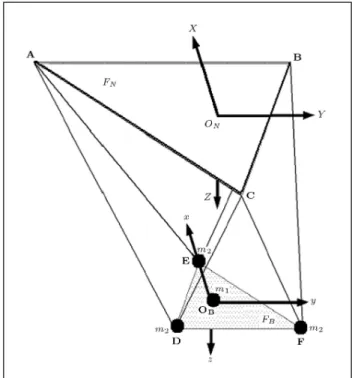
MATHEMATICAL MODELING OF CDRS In this study, the well-known NIST robocrane, as a 6 d.o.f cable driven robot, was considered. This robot is an inverted Stewart platform, in which rigid legs are replaced by cables. Its suspended movable platform (or end-eector) and xed support are two equilateral triangles, as shown in Figure 1.

The end-eector is kinematically constrained by maintaining tension in all six cables, which terminate in pairs at the vertices of the xed support. The orientation and position of the end-eector are deter-mined by a six-actuator system, in which each cable is controlled separately. In order to study the kinematics and dynamics of a robocrane, two frames are used:

Figure 1. Free-body diagram for the robocrane with point masses.

1. The inertial coordinate, FN, with its origin in the

center of the xed support (with vertices A, B and C).

2. The body coordinate, FB, which is similarly

con-nected to the center of mass of the end-eector (with vertices D, E and F ).

Here, fqg is introduced as follows:

fqg = [xD; yD; zD; xE; yE; zE; xF; yF; zF]: (1)

The elements of generalized coordinates fqg are the Cartesian coordinate of vertices of the end-eector, as written in the reference coordinate. These generalized coordinates are not independent and, since the robot has six degrees of freedom, three constraint equations are necessary. These constraint equations are as follows:

8 > < > :

(xD xE)2+ (yD yE)2+ (zD zE)2= (2b)2

(xE xF)2+ (yE yF)2+ (zE zF)2= (2b)2

(xD xF)2+ (yD yF)2+ (zD zF)2= (2b)2(2)

In order to derive kinetic and potential energies, in terms of the discussed generalized coordinates, it will be easy to use point masses instead of distributed mass. Otherwise, complex terms will appear in the rotational part of the kinetic energy. As shown in Figure 1, four point masses are located instead of a distributed mass in the end-eector: a single point mass (m1) at the

center of the mass and three identical masses (m2) at

the vertices of the end-eector. By considering the inertia specication of these systems, (m1) and (m2)

can be determined as follows: (

m1+ 3m2= m

2m2b2= Ixx ) m1= 9m2=

3

4m: (3)

The kinetic and potential energies of the robot are derived in terms of the discussed generalized coordi-nates. The general dynamic equations of motion can be obtained from Lagrangian formulation [10]:

d dt

@K(q; _q) @ _q

@K(q; _q)

@q +

@V (q) @q

= Qi+ 3

X

j=1

Jcij;

i = 1; 2; ; 9: (4)

It leads to;

[D(q)]99fqg91+ fGg91= fQg91

[p]T

96fT g61 [Jc]T93fg31: (5)

Equation 5 is written in the following form:

[D(q)]fqg + fGg fQg = [J]

T

; (6)

where [D(q)] is the inertia matrix, fG(q)g is the gravity vector, [J(q)] is the Jacobian matrix, fT g is the vector of cables tension and fg is the Lagrange multiplier vector.

Since the dynamic modeling of CDRs is concerned with relating the motion end-eector to the required active actuator torque, the forces in the cables are derived using the dynamic equations of the end-eector and actuators. In this paper, the dynamic behavior of the lumped actuators (each actuator includes a motor and pulley system) is also considered. The free body diagram for the ith actuator is shown in Figure 2.

The combined motor and cable pulley dynamics equations can be expressed as [11]:

evl= r:T; (7)

evl= Ja:  + Ca: _; (8)

where r is the identical cable pulley radius for each actuator. The lumped actuator rotational inertias for each actuator and the viscous damping coecients at

Figure 2. Free-body diagram for the ith actuator [11].

each motor shaft are also included to provide a linear model for the system friction with:

Ja = diag(J1; ; Jm); (9)

Ca= diag(C1; ; Cm): (10)

In this case study, the dynamic equation is given as follows:

n r

o

= [JT_{]:r: [D]fqg + fGg}

+

1 r

[pT_]fJ

a + ca_g

!

: (11)

LINEARIZATION OF THE STATE SPACE DYNAMIC EQUATION

In order to obtain the numerical solution of the non-linear constrained trajectory optimization problem, in order to increase the load carrying capacity, dynamic Equation 11 can be rewritten as:

q =

r:[D(q)] + [p]T_J a:

@ @q

1

:Jn _ro [p]T_J

a_dtd

@ @q

_q + Ca_

rfGg

= f(~q; ~_q; ; mL): (12)

By dening the state vector as q = [x1; x2]T, where

x1 = (q1; q2; ; qn)T and x2 = ( _q1; _q2; ; _qn)T,

~_q = ~_x1

~_x2

=

~ x2

f( ~X(j); ~(j); mL)

= ~F ( ~X(j); ~(j); mL): (13)

Equation 13 is the state space representation of the dynamic Equation 12, where ~X is a 2n 1 vector and f(X; ; mL) consists of n nonlinear functions. The

dis-cretized form of the state space dynamic Equation 13 is:

~

X(j + 1) X(j)~

h = ~F ( ~X(j); ~(j); mL); (14) where h = (tf ti)

m , tf, ti are the start and end time

of the robot motion and m is the number of set points used to discretize the end-eector trajectory. The nonlinear function, f(X; ; mL), at the (k + 1)th

trajectory, is expanded in a Taylor series about the (k)th trajectory. After neglecting the higher order (nonlinear) terms, the following equation is obtained:

~

X(j+1) = [Gj] ~X(j)+[Hj](j)+ ~BjmL+ Dj; (15)

where the matrices [Gj], [Hj] and j, Dj vectors are

given in [13].

X(j + 1) can be written as a linear combination of the load mL and the torque ~(i), i = 1; 2; 3; ; j.

Equation 15 then becomes: ~

X(j + 1) = ~Xh(j + 1) + ~jmL+ j

X

i=1

[ji](i);

j = 1; 2; ; m: (16)

This equation is the basic linearized dynamic equation, where:

~

Xh(1) = ~X(t1); (17)

~

Xh(j + 1) = [Gj] ~Xh(j) + ~Dj; (18)

~1= ~B1; (19)

~1= [Gj]~j 1+ ~1; (20)

[aji] = [Gj][aj 1;i];

for i < j; (21)

[aji] = [Hj];

for i = j: (22)

FORMULATION OF THE OPTIMIZATION PROBLEM

In this section, the complete problem formulation is presented for synthesizing dynamic robot motion

with maximum load carrying capacities. The com-plete formulation of such a problem is given be-low:

1. The robot geometric parameters and the mass of the end-eector;

2. The initial and nal states: ~x1(ti) = ~q(ti) = ~x1i;

x2(ti) = ~o; (23)

~x1(tf) = ~q(tf) = ~x1f;

x2(tf) = ~o; (24)

where o is an n 1 null vector; 3. Total cycle time, rT = tf ti.

Constraints of problem:

1. The state space Equation 13 should be satised; 2. The joint actuator torques constraint:

~min( ~X(j)) ~(j) ~max( ~X(j)); (25)

where ~min( ~X(j)) and ~max( ~X(j)) are in general

nonlinear functions representing the torque-speed characteristics of the actuators;

3. The workspace constraint:

~x₁ ~x1(t) ~x+1: (26)

At the moment of moving of the end-eector, it is bounded to be within the limitation of the robot workspace. The generalized coordinate, assumed to be chosen from inside the 3D volume [10], is the workspace limitation. x+

1 and x1 are the upper and

lower bound of the generalized coordinates, respec-tively. The obtained optimal trajectory should not exceed this limitation, because this causes cables to lose their positive tensions;

4. The upper bound of payload m+

L: That is the

smaller value of the static load carrying capacity calculated at the two end positions.

The objective function is maximizing the dynamic load carrying capacities, mL, along with nding the

optimal trajectory, x_(t).

The trajectory synthesis formulation is a non-linear optimization problem. It is written in a form slightly dierent from a general optimal control prob-lem, where the objective function has an integral form. In the above formulation, the objective function consists of a single variable, mL, which is not a function

for the entire trajectory. It should be pointed out, however, that mLis implicitly included in the nonlinear

state space equation.

ITERATIVE LINEAR PROGRAMMING (ILP) FORMULATION

The ILP method uses linear programming to solve the linearized equations for each iteration. The linear programming problem can be formulated as follows.

At rst, the nal state reaching the condition from Equation 16 can be obtained as:

~

X(m + 1) = ~Xh(m + 1) + ~mmL

+Xm

i=1

[ami]~(i)=X(tf): (27)

Equation 27 can be written as:

~mmL+ [E]~ = ~X(tf) X~h(m + 1); (28)

where:

[E] =[m1] [m2] [mm]2 R(2nnm);

(29)

~ =~(1); ~(2); ; ~(m)2 R(nm1)_{: (30)}

It should be noted that [E] and Xh(m+1) in the above

equation are computed based on the values of the state and control variables of the previous iteration. Since X(tf) is also given, the only unknowns in Equation 28

are mL and ~ vectors. In order to facilitate the LP

solution, Equation 28 can be written by two sets of inequalities.

~mmL+ [E]~m ~e

~X(tf) X~h(m + 1); (31)

~mmL+ [E]~m+ ~e

~X(tf) X~h(m + 1); (32)

where ~e = [epos1; epos2; ; evel1; evel2; ]T is a 2n

vector, and the rst n elements (epos) represent the

nal position error tolerances, and the last n elements (evel) represent the velocity error tolerances. This

modication introduces two more variables (epos; evel)

and 2n inequality constraints. If actuators are per-manent magnet DC motors, the torque-speed charac-teristic function, ~min( ~X(j)) and ~max( ~X(j)), can be

approximated by the following equations: ~(j) ~max( ~X(j)) = ~K1 [K2] _(j);

j = 1; 2; ; m; (33)

~(j) ~min( ~X(j)) = ~K1 [K2] _(j);

j = 1; 2; ; m; (34)

where k1= stall is an n1 constant vector, k2= stall_!0

is an n n diagonal constant matrix obtained from the equivalent motor constants and !0is the maximum

no-load speed of the actuator. The \max" or \min" in the superscripts indicates whether the actuator is saturated at its upper or lower bound. Note that both stall torques and the maximum no-load speed of the actuators must be specied in order to determine an actuator torque bound.

The main drawback of CDRs is the unilateral actuation imposed by the cables. Since cables can only apply tensile force, this limitation can cause excessive deviation from the prescribed trajectory, even if the joint torque constraint is not violated. A more successful approach should maximize the load-carrying capacity and allowable cable tension bound attained for the end-eector trajectory. The desired trajectory is characterized as the set of points that the centroid of the end-eector can reach with tensions in all suspension cables. The following assumption is used for the points on the trajectory:

1. The maximum tension is considered for all cables. 2. The cables must be capable of exerting a positive

wrench on the platform. All cable tensions must be non-negative to equilibrate the end eector for an applied force.

3. All active cables must remain in tension to be eective for the equilibrium or dynamic motions. The feasible points are specied by imposing the following inequalities [12]:

0 Ti Tmax; i = 1; :::; m: (35)

In a pseudostatic condition, the tension in the cables is equal or greater than ~min( ~X(j))=r. When

the dynamic eects are considered, one or more cable can become slack, despite a positive ~min( ~X(j)), and

online cable tension estimation is needed. Referring to the dynamic term, Equation 7 claried that higher minimum torques are needed. If the bias term, vel,

is positive, all cable force components are forced to be zero at the minimum. It can be shown that, for each actuator, ~min( ~X(j)) = vel. If vel were negative,

the minimum torque required to ensure that the cor-responding cable was in tension could be negative for

one or more actuators, since all torque actuators were forced to be positive. Therefore, constraints are needed for the online actuator torques control, which can be written as follows:

~min( ~X(j)) = maxfvel; 0g: (36)

Writing these constraints in matrix form leads to:

~ ~bu=

~

K1 [K2]~_k(1)

~

K1 [K2]~_k(2)

... ~

K1 [K2]~_k(m)

; (37)

~ ~bl= maxfvel; 0g; (38)

where ~bland ~bu are, respectively, the lower and upper

bound vectors of the actuators. By a change of variables, as below, the problem can be converted to a standard linear programming problem:

~Y = ~bu ~; or ~ = ~bu ~Y ; ~Y 0: (39)

Substituting Equation 39 into Equation 37 leads to:

~Y ~bu ~bl: (40)

Using Equation 16, the workspace constraint is given by Inequality 26 written as:

~x₁ X~1h(j + 1) ~1jmL+ j

X

i=1

[a1ji]~(i)

~x+

1 X~1h(j + 1);

j = 1; 2; ; m; (41)

where 1j, X1h(j + 1) are the upper n 1 vectors

of j and Xh(j + 1), respectively, and [1ji] is the

upper n n sub-matrix of [ji]. Equation 41 can

be written in the following form by letting [Aj] =

[1j1; 1j2; ; 1jj; 0; 0; ; 0] and rearranging terms

which can be written as follows:

~1jmL [Aj]~Y ([~x1+ X~1h(j + 1)] [Aj]~bu);

j = 1; 2; ; m; (42)

~1jmL+ [Aj]~Y ([ ~X1h(j + 1) ~x1] + [Aj]~bu);

j = 1; 2; ; m; (43)

where [Aj] is a n nm matrix.

As mentioned above, the upper bound of load m+

L is determined from SLCC (Static Load Carrying

Capacity) at the two end points. Since the robot must

completely stop at the two end points, the maximum DLCC for the trajectory cannot be greater than the SLCC at either one of the end positions. This means that:

m+

L = minfmSLi; mSLfg; (44)

and:

mL m+_L; (45)

where mSLi and mSLf are the SLCC at the initial

and nal positions, respectively. Combining all the constraints and writing the result in a matrix form gives: 2 6 6 6 6 4

1 0 0

[0] [1](nmnm) [0]

1j(nm1) [Aj](nmnm) [0]

m(2n1) [E](2nnm) [I](2n2n)

m(2n1) [E](2nnm) [I](2n2n)

3 7 7 7 7 5 8 < : mL ~Y(nm1) ~e(2n1) 9 = ; 8 > > > > > < > > > > > : m+ L

~Ylim it(nm1)

~

Xlim it(nm1)

~ X+ f ~ X_f 9 > > > > > = > > > > > ; : (46)

And the dimensions of the matrices and vectors are as follows:

[(2nm + 4n + 1) (2n + nm + 1)] f(2n + nm + 1) 1g

f(2nm + 4n + 1) 1g; (47)

where 1j, [Aj] and Xlim it can be obtained from

Inequalities 42 and 43 using the method described above, and:

~Ylim it = ~bu ~bl;

~ X+

f = [X(tf) Xh(m + 1)] [E]bu;

~

X_f = [Xh(m + 1) X(tf)] + [E]bu:

The objective function of this LP problem is dened as:

Z = maxfCT_{V g; (48)}

where C = [1; 0; 0; ; Wpos; Wvel] with Wpos; Wvel

> 0 (weighting factors) and ~V = [mL; ~Y ; ~epos;~evel] with

~Y 0.

The load carrying capacity, mL, can be

maxi-mized by this objective function, and simultaneously the position and velocity errors at the end points of the trajectory are minimized. Since the objective function (Equation 48) and the constraints equation (Equation 46) are both linear, we have a standard linear programming problem.

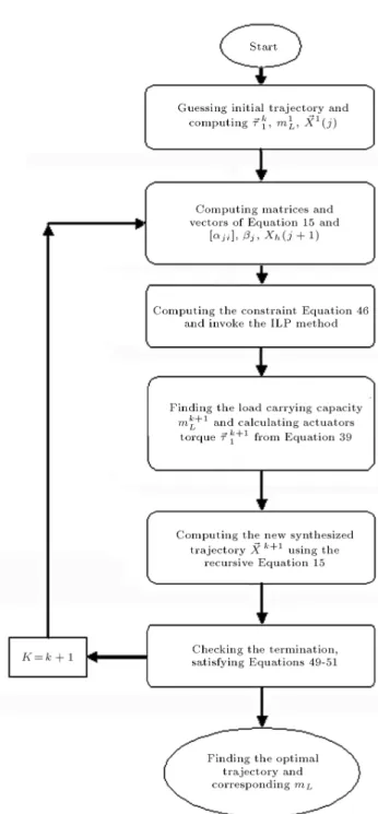
COMPUTATIONAL ALGORITHM

The computing method for the optimal trajectory problem is formulated, as shown in Figure 3. First, initialize the trajectory. This step involves guessing an initial control and state variable trajectory. A good initial guess may be obtained by using polyno-mial trajectories to connect the two end points. By discretizing the initial trajectory into m set points, the corresponding linearized constraint coecients are computed and, then, an iterative linear programming subroutine is invoked to update mL, ~Y and ~e. Using

these updated variables, the new trajectory, Xk+1_(j),

is synthesized. Then, the termination conditions are checked:

maxfepos; evelg "e; (49)

maxfj ~Xk+1_{(j) X~}k_{(j)j; j = 2; ; mg "}

x; (50)

mk+1

L mkL "m; (51)

where "e; "x and "m are predened small positive

constants. If the termination conditions are satised, then, the updated trajectory is optimal, and the corresponding value of mL is the maximum

allow-able load that can be carried by the callow-able driven robot. Otherwise, the program jumps to step 2 in ILP method owchart shown in Figure 3. Also, satisfying the termination criterion means that lin-earization errors are eliminated (or signicantly re-duced) when the ILP method converges to the optimal solution.

In general, because of the discretization (trunca-tion) error of the dierence equation, the continuous state space equation will be satised only if the time interval is \suciently small".

SIMULATION

A simulation study is presented to investigate the application and eciency of the proposed algorithm. A cable driven robot with 6 d.o.f is considered, as shown in Figure 1 [13].

For simulation, a cable driven robot must carry a load from an initial point with coordinate X0 = [ 0:1; 0:1; 1:5; 0; 0; 0] to the nal point in the robot workspace with coordinate XF = [0:1; 0:1; 1:8; 0; 0; 0], during overall time tf = 1 s. The velocities and

accelerations at the start and end points are zero. The path parameter unknowns are determined, so that the initial and nal conditions are satised. The trajectory used for an initial guess in simulation is a polynomial of the fth order. In this simulation, it is assumed that there is no exerted external wrench on the robot.

Figure 3. ILP method owchart for computing optimal trajectory.

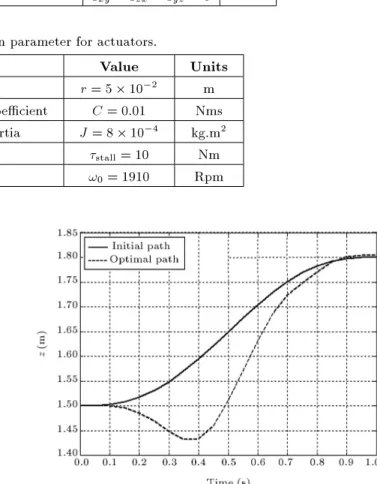
Geometrical and mechanical characteristics used in the simulation are listed in Table 1 and the other used parameters relative to the robot actua-tors, consisting of motors and pulleys, are given in Table 2.

By discretizing the trajectory to m = 20 set points, the procedure for synthesizing the optimum trajectory converged after eleven iterations, and the maximum allowable carrying load without violating either of the constraints is mL= 75:52 kg.

Figure 4 gives the trajectory of the center of mass of the end-eector for the optimal trajectory and initial

Table 1. Geometrical parameters of robot.

Parameter Value Units End-eector mass m = 15 kg Half of the side of the upper triangle (xed base) a = 0:3p3 m Half of the side of the lower triangle (end-eector) b = (1=2)a m

Ixx= Iyy= mb₆2

Moment of inertia (end-eector) Izz= 2Ixx kg.m2

Ixy= Izx= Iyz= 0

Table 2. Simulation parameter for actuators.

Parameter Value Units Pulley radius r = 5 10 2 _m

Motor shaft viscous damping coecient C = 0:01 Nms Lumped actuator rotational inertia J = 8 10 4 _kg.m2

Stall torque stall= 10 Nm

Maximum no-load speed !0= 1910 Rpm

Figure 4. Motion of center of mass of end-eector on x y coordinates.

guess in the xy plane. Figure 5 shows the variation of the z coordinate in time. The initial and nal optimal positions and velocities of the vertices of the end-eector that are used as generalized coordinates in the dynamic equations can be depicted. One of them is shown in Figure 6. Figure 7 gives the linear programming solution of mL at each iteration. The

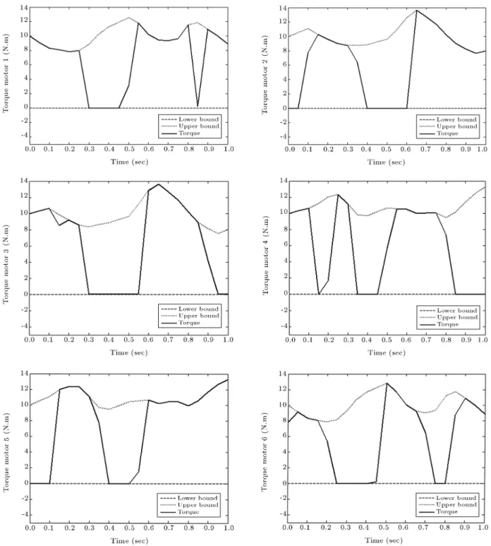
corresponding initial path and the nal optimal path in Cartesian 3D space are given in Figure 8. Figure 9 presents the optimal torques related to the optimal trajectory with regard to the upper and lower bounds of the actuator torque.

As mentioned above, in the linearization pro-cess of the ILP method, the higher order (nonlinear) terms in the Taylor series are neglected and because CDRs have nonlinear dynamics, errors as a result

Figure 5. Motion of center of mass of end-eector on z-coordinates.

of neglecting higher order terms will exist in the solution process. Tensions of cables are computed for dierent masses from an initial guess until optimal trajectory during the process of obtaining the opti-mal trajectory for ensuring robot stability. Also, as mentioned above, Equation 38 causes the actuators torque to be a non-negative value. Regarding the optimal trajectory and corresponding actuators torque variations, it is realized that, while the end eector moves along the optimal trajectory, the coupling inertia of the load is minimized. Simultaneously, at most parts of the trajectory, actuators work close to their maximum torque capacity, and the actuators torques have a non-negative value in total operating time, resulting in an increase in the conveyable load of the CDR.

Figure 6. Position and velocity of vertex D.

Figure 7. Optimal maximum dynamic payload in each iteration.

CONCLUSION

In this paper, a computational algorithm is developed to obtain a numerical solution to the optimization problem associated with synthesizing optimal trajec-tories in CDRs. This was achieved by torque capacity constraints in addition to considering the workspace constraint of a robot. A simulation case study of

Figure 8. Initial and optimal trajectory in 3D view.

CDR was presented to investigate the eciency of the algorithm. It is seen that, while the CDR moves along the optimal trajectory, the coupling inertia of the mass is minimized without violating either of the constraints. Moreover, during the motion, actuators are working with full or near to full capacity. As understood from the simulation, the load carrying capacity is increased from an initial value 15 kg to mL= 75:52 kg.

Figure 9. Optimal torques of six motors related to optimal trajectory.

ACKNOWLEDGMENT

The authors gratefully acknowledge the support of the School of Mechanical Engineering at the Iran Univer-sity of Science & Technology. Support for this research is also provided by the IUST Research Program.

REFERENCES

1. Albus, J., Bostelman, R. and Dagalakis, N. \The NIST robocrane", J. Robot Syst., 10, pp. 709-724 (1993).

2. Alp, A. and Agrawal, S. \Cable suspended robots: design, planning, and control", Proceedings of IEEE Int. Conf. on Robotics and Automation, Washington, pp. 4275-4280 (2002).

3. Wang, L.T. and Ravani, B. \Dynamic load carrying ca-pacity of mechanical manipulators: II. Computational procedure and applications", J. Dyn. Syst. Meas. Control, 110, pp. 53-61 (1988).

4. Korayem, M.H. and Ghariblu, H. \Maximum allowable load of mobile manipulators for two given end points

of end eector", Int. J. Adv. Manuf. Technol., 24, pp. 743-751 (2004).

5. Korayem, M.H. and Nikoobin, A. \Formulation and numerical solution of robot manipulators in point-to-point motion with maximum load carrying capacity", Scientia Iranica. Trans. B, 16(1), pp. 28-38 (2009). 6. Korayem, M.H. and Bamdad, M. \Dynamic

load-carrying capacity of cable-suspended parallel manipu-lator", Int. J. Adv Manuf. Technol., 44(7-8), pp. 829-840 (2009).

7. Yue, S., Tso, S.K. and Xu, W.L. \Maximum dynamic payload trajectory for exible robot manipulators with kinematic redundancy", Mech. Mach. Theory, 36, pp. 785-800 (2001).

8. Korayem, M.H., Haghpanahi, M. and Heidari H.R. \Maximum allowable dynamic load of exible manipu-lators undergoing large deformation", Scientia Iranica, Trans. B, 17(1), pp. 61-74 (2010).

9. Korayem, M.H. and Shokri, M. \Maximum dynamic load carrying capacity of a 6UPS-Stewart platform manipulator", Scientia Iranica, 15(1), pp. 131-143 (2008).

10. Afshari, A. and Meghdari, A. \New Jacobian matrix and equations of motion for a 6 d.o.f cable-driven robot", Int. J. of Advanced Robotic Systems, 4(1), pp. 63-68 (2007).

11. Gallina, P., Rossi, A. and Williams, R.L. \Planar cable-direct driven robots: dynamic and control", Pro-ceedings of the ETC2001/ASME Design Engineering Technical Conference, Pittsburgh, PA, USA (2001). 12. Fattah, A. and Agrawal, S.K. \On the design of

cable-suspended planar parallel robots", J. of Mech. Des., 127, pp. 1021-1028 (2005).

13. Naja, Kh. \Dynamic analysis of cable driven robots in the presence of the exibility and nding dynamic load carry capacity on optimal trajectory", MSc thesis, College of Mechanical Engineering, Islamic Azad Uni-versity, Science and Research Campus, Tehran (2009).

BIOGRAPHIES

Moharam Habibnejad Korayem was born in Tehran, Iran on April 21, 1961. He received his BS (Hon) and MS in Mechanical Engineering from the Amirkabir University of Technology in 1985 and 1987, respectively, and his PhD degree in Mechanical Engi-neering from the University of Wollongong, Australia, in 1994. He is a Professor in Mechanical Engineering at the Iran University of Science and Technology and has been involved with teaching and research activities in robotics at the Iran University of Science and Technology for the last 15 years. His research interests include dynamics of elastic mechanical manipulators, trajectory optimization, symbolic modeling, robotic multimedia software, mobile robots, industrial robotics standards, robot vision, soccer robot, and analysis of mechanical manipulators with maximum load carrying capacity. He has published and presented more than 300 papers in international journals and conferences in the eld of robotics.

Khaled Naja was born in Meyaneh, Iran on Septem-ber 10, 1983. He received his BS and MS (Hon) in Mechanical Engineering from the Islamic Azad University of Tehran in 2006 and 2009, respectively. His research interests include robotic systems, linear programming, parallel manipulators, industrial au-tomation and mechatronic systems.

Mehdi Bamdad was born in Sabzevar, Iran on June 13, 1982. He received his BS in Mechanical Engineering from KNT University of Technology in 2004 and a MS from Semnan University in 2006. He is a PhD candidate in Mechanical Engineering at the Iran University of Science and Technology. His research interests include robotic systems, optimization, parallel manipulators, industrial automation and mechatronic systems.