Sharif University of Technology
Scientia IranicaTransactions A: Civil Engineering www.scientiairanica.com
Adaptive node moving renement in discrete least
squares meshless method using charged system search
H. Arzani
a, A. Kaveh
b;and M. Dehghan
aa. Department of Civil Engineering, Shahid Rajaee Teacher Training University, Tehran, P.O. Box 16785-136, Iran.
b. Centre of Excellence for Fundamental Studies in Structural Engineering, Iran University of Science and Technology, Narmak, Tehran, P.O. Box 16846-13114, Iran.
Received 22 December 2012; received in revised form 11 October 2013; accepted 27 January 2014
KEYWORDS Charged system search;
Discrete least squares; Adaptive renement; Planar elasticity problems.
Abstract. Discrete Least Squares Meshless (DLSM) method has been used for the solution of dierent problems ranging from solid to uid mechanics problems. In DLSM method the locations of discretization points are random. Therefore, the error of the initial solution is rather high. In this paper, an adaptive node moving renement in DLSM method is presented using the Charged System Search (CSS) for optimum analysis of elasticity problems. The CSS algorithm is eectively utilized to obtain suitable locations of the nodes. The CSS is a multi-agent optimization technique based on some principles of physics and mechanics. Each agent, called a Charged Particle (CP), is a sphere with uniform charge density that can attract other CPs by considering the tness of the CP. To demonstrate the eectiveness of the proposed method, some benchmark examples with available analytical solutions are used. The results show an excellent performance of the CSS for adaptive renement in meshless method.
© 2014 Sharif University of Technology. All rights reserved.
1. Introduction
Finite element method has been successfully used for the simulation of a large variety of practical engineering problems in the last decades. The method, however, involves some diculties for certain processes such as creak propagation, extremely large deformation or implementation of adaptivity due to the need for mesh moving or remeshing of the domain. In the last decade several methods referred to as meshless method have been proposed and used to overcome these problems. Recently, a new meshless method which utilizes strong formulation of the governing dierential equations, named Discrete Least Squares Meshless (DLSM) method [1], was proposed and used for the solution of Poisson equation. The advantages
*. Corresponding author. Tel.: +98 21 77240104; Fax: +98 21 77240398
E-mail address: [email protected] (A. Kaveh)
of this method over other numerical methods are no need for integration, simplicity of use and symmetric matrix of coecients. The method has been used for the seepage problems [2], solution of solid mechanics problems [3] and many other cases, and its eectiveness has been proven. In all numerical methods such as nite element and meshless methods, adaptive rene-ment has become a standard procedure to achieve the desired accuracy by using a minimum number of nodes. An ideal computational algorithm with the re-meshing ability and pointing should be in such way that the density of nodes or new mesh increases in locations with higher computational errors. Formerly methods for an error estimation and adaptive renement for hyperbolic problems in one-dimensional case [4], node enrichment adaptive method [5] in which more nodes are added in the regions with higher errors, and node moving strategy based on spring analogy [6] in DLSM method have been developed. These methods, however, have high computational costs due to the new
added nodes or nding new locations of the previous nodes.
To resolve these shortcomings, meta-heuristic al-gorithms can be used. Meta-heuristic alal-gorithms are more suitable than traditional methods of optimiza-tions and adaptivity due to their capability of exploring and nding promising regions in the search space in an aordable time and less computational costs. One of the best searching algorithms and more e-cient than other optimizing algorithms is the Charged System Search (CSS). The algorithm that is based on electrostatics and Newtonian mechanics has been proposed by Kaveh and Talatahari [7]. The CSS has been used for a large variety of optimization problems such as optimal design of frame structures, optimum grillage system design, truss optimization and design optimization of reinforced concrete 3D structures [8-11]. The CSS for minimax and minisum facility layout problem [12] is one of the new researches which shows the applicability and robustness of the CSS for the problem of nding suitable locations. In this paper a node moving adaptive renement strategy with the use of the CSS algorithm is presented for solving problems in solid mechanics. The process is very eective and because of the resolving the limitations of meshing and remeshing in meshless methods, the process is much more exible and ecient than other adaptive renement methods in FEM and meshless methods. Sections 2 and 3 present the fundamental concepts of DLSM method and CSS algorithm, respectively. In Section 4, error estimation and an adaptive renement is exhibited. Section 5 illustrates the capabilities of the proposed method through some benchmark examples, where the results are compared with the available analytical solutions. Finally, some concluding remarks are addressed in Section 6.
2. Discrete Least Squares Meshless (DLSM) 2.1. Moving least squares shape functions Among the available meshless approximation schemes, the Moving Least Squares (MLS) method [13] is gen-erally considered to be one of the best methods to interpolate random data with a reasonable accuracy, because of its completeness, robustness and continu-ity [14,15]. With the MLS interpolation, the unknown function (x) is approximated by:
(x) =Xm
i=1
Pi(x):i(x) PT(x):(x): (1)
Here, P (x) is a polynomial basis in the space coor-dinates, and m is the total number of the terms in the basis. For a 2D problem we can specify P (x) = [1 x y x2 xy y2] for m = 6. (x) is the vector
of coecients and can be obtained by minimizing a
weighted discrete L2 norm as:
J =
n
X
j=1
W (x xj):PT(xj):(x) ~uj2; (2)
where n is the number of nodes in the domain, and ~uj
is the nodal value of the function to be approximated at point xj. The weight function W (x xj) is usually
built in such a way that it has the following properties: W (x xj) > 0 within the support domain,
W (x xj) = 0 outside the support domain,
W (x xj) monotonically decreases from the
point of interest at x, and
W (x xj) is suciently smooth, especially on
the boundary of j.
Here, for a better performance in meshless method, the cubic spline weight function is employed, given by:
W (x xj) = W ( d) =
8 > < > :
2
3 4 d2+ 4 d3 for d 12 4
3 4 d + 4 d2 43d3 for 12 < d 1
0 for d > 1 (3) where d = (x xj)=dw and dw is the size of inuence
domain of point xj. Minimization of Eq. (2) with
respect to the coecient (x) leads to:
(x) = PT(x)A 1(x)B(x)h; (4)
where: A(x) =
n
X
j=1
W (x xj)P(xj)PT(xj); (5)
and: B(x) =
W (x x1)P(x1); W (x x2)
P(x2); :::; W (x xn)P(xn)
: (6)
Eq. (4) can be written in the compact form: (x) =
n
X
i=1
NT
i (x)i(x) = NT(x)h; (7)
leading to the denition of MLS shape function dened as:
NT(x) = PT(x)A 1(x)B(x); (8)
where NT(x) contains the shape functions of nodes at
point x, which are called Moving Least Squares (MLS) shape functions.
2.2. Discrete least squares meshless method Consider the following partial dierential equation:
8 > > > < > > > :
L() + f = 0 in B() t= 0 in t
= 0 in u
(9)
where L and B are partial dierential operators, and t are vectors of prescribed displacements and tractions on the Dirichlet and Neumann boundaries, respectively; is the considered domain; uand tare
the displacement and traction boundaries, respectively; f is the vector of external force or source term on the problem domain.
Suppose the value of the estimating function in a point such as xk is denoted as:
(xk) = m
X
i=1
Ni(xk)i: (10)
According to the discretization of the problem domain and its boundaries, using Eq. (4), the residual of partial dierential equation at point xk is obtainable as:
R(xk) = L ((xk)) + f(xk); k = 1; :::; M: (11)
The residual of Neumann boundary condition at point xk on the Neumann boundary can also be presented
as:
Rt(xk) = B ((xk)) t(xk); k = 1; :::; Mt: (12)
Finally the residual of Dirichlet boundary condition at point xk on the Dirichlet boundary can be written
as:
Ru(xk) = (xk); k = 1; :::; Mu; (13)
where Md is the number of internal points, Mt is the
number of points on the Neumann boundary, Mu is
the number of points on the Dirichlet boundary, and M is the total number of points. A penalty approach can now be used to form the least squares functional of the residuals dened as:
J =12 "M
d
X
k=1
R2
(xk)+: Mt
X
k=1
R2
t(xk)+: Mu
X
k=1
R2 u(xk)
# ;
(14) where and are the penalty coecients for the importance of Neumann and Dirichlet boundary conditions, respectively. Minimization of the functional with respect to nodal parameters (i; i = 1; 2; :::; n)
leads to the system of equations:
K = F; (15)
where:
Kij= M
X
k=1
[L(N)]Tk [L(N)]k+
Mt
X
k=1
[B(N)]Tk [B(N)]k
+ XMu
k=1
[N]T kk;
(16)
Fi= M
X
k=1
[L(N)]Tk[L(N)] fk+ Mt
X
k=1
[B(N)]Tk tk
+ XMu
k=1
[N]T kk:
(17) The stiness matrix K in Eq. (16) is square, symmetric, and positive denite. Therefore the nal system of equations can be solved directly via ecient solvers.
3. Charged system search
The charged system search is based on electrostatics and Newtonian mechanics laws. The Coulomb and Gauss laws provide the magnitude of the electric eld at a point inside and outside a charged insulating solid sphere, respectively, as [16]:
Eij =
8 < :
keqi
a3 rij if rij < a
keqi
r2
ij if rij a
(18)
where keis a constant known as the Coulomb constant,
rij is the separation of the centre of sphere and the
selected point, qiis the magnitude of the charge, and a
is the radius of the charged sphere. Using the principle of superposition, the resulting electric force due to N charged spheres is equal to [7]:
Fj= keqj N
X
i=1
qi
a3rij:i1+
qi
r2 ij:i2
! ri rj
ri rj;
8 < :
i1= 1; i2= 0 () rij < a
i1= 0; i2= 1 () rij a
(19)
Also, according to Newtonian mechanics, we have [16]: r = rnew rold; (20)
V = rnew rold
t ; (21)
a = VnewtVold; (22) where roldand rneware the initial and nal positions of
and a is the acceleration of the particle. Combining the above equations and using Newton's second law, the displacement of any object as a function of time is obtained as:
rnew= 12mF:t2+ vold:t + rold: (23)
Inspired by the above electrostatics and Newtonian mechanics laws, the pseudo-code of the CSS algorithm is presented as follows [7].
Level 1: Initialization
Step 1. Initialization. Initialize the parameters of the CSS algorithm. Initialize an array of Charged Particles (CPs) with random positions. The initial velocities of the CPs are taken as zero. Each CP has a charge of magnitude dened considering the quality of its solution as:
qi= tbest tworstt(i) tworst ; i = 1; 2; :::; N; (24)
where tbest and tworst are the best and the worst tness of all the particles, and t(i) represents the tness of agent i. The separation distance rij between
two charged particles is dened as:
rij = (X Xi Xj
i+ Xj)=2 Xbest+ "; (25)
where Xi and Xj are the positions of the ith and
jth CPs, respectively, Xbest is the position of the best
current CP, and " is a small positive number to avoid singularities.
Step 2. CP ranking. Evaluate the values of the tness function for the CPs, compare with each other and sort them in increasing order.
Step 3. CM creation. Store the number of the rst CPs equal to Charged Memory Size (CMS) and their related values of the tness functions in the Charged Memory (CM).
Level 2: Search
Step 1. Attracting force determination.
Determine the probability of moving each CP toward the others considering the probability function:
pij =
8 < :
1 t(i) tbestt(i) t(j) >rand _ t(j)>t(i)
0 else (26)
and calculate the attracting force vector for each CP as:
Fj=qj N
X
i;i6=j
qi
a3rij:i1+
qi
r2 ij:i2
!
pij(Xi Xj)
8 > > > < > > > :
j = 1; 2; :::; N
i1= 1; i2= 0 () rij < a
i1= 0; i2= 1 () rij a
(27)
where Fj is the resultant force aecting the jth CP.
Step 2. Solution construction. Move each CP to the new position and nd its velocity using the following equations:
Xj;new=randj1:ka:mFj j:t
2
+ randj2:kv:Vj;old:t + Xj;old; (28)
Vj;new=Xj;newtXj;old; (29)
where randj1 and randj2 are two random numbers
uniformly distributed in the range (0,1), t is the time step, and it is set to 1. kais the acceleration coecient,
kv is the velocity coecient to control the inuence of
the previous velocity. Here, ka and kv are taken as
0.5. Also, mj is the mass of the CPs, which is equal to
qj in this paper. The mass concept may be useful for
developing a multi-objective CSS.
Step 3. CP position correction. If each CP exits from the allowable search space, correct its position using the HS-based handling approach as described for the HPSACO algorithm [17,18].
Step 4. CP ranking. Evaluate and compare the values of the tness function for the new CPs, and sort them in an increasing order.
Step 5 CM updating. If some new CP vectors are better than the worst ones in the CM, in terms of their objective function values, include the better vectors in the CM and exclude the worst ones from the CM. Level 3: Controlling the terminating criterion Repeat the search level steps until a terminating criterion is satised.
4. Error indicator and adaptive renement Adaptivity is an important tool for the eciency and eectiveness of any numerical method. Any adaptive
procedure is formed of two main parts, error estimation and mesh renement. For any successful adaptive pro-cedure, an actual error estimator is essential. Dierent methods to estimate error have been introduced and applied in the numerical methods. These methods can be separated into two categories. Methods based on residual of the dierential equations governing on the problem [19,20] and the methods based on the restoration of the error which considered the error as the gradient of the solution [21,22]. In this study, error estimation based on least squares function formed from weighted residuals is used [23], where the error for each point is dened as:
ek=
r 1
2[R2(xk) + :R2t(xk) + :R2u(xk)]: (30)
Here, ek is the error of any point in the problem
domain or its boundaries. The advantage of this choice is the availability of the error estimator in the process of the main simulation. Dierent methods for renement and achieving more accurate solutions after identifying the error distribution can be used. There are three general methods of renement in nite element: mesh moving (r-method), mesh enrichment (p-method) and p-renement whereby higher order shape functions are used. In mesh moving methods the number of the nodes is constant but the location of the nodes is altering according to the achieved errors. In FEM the connectivity of the nodes may be disturbed and some of the elements can overlap or be zero area. Therefore there is some limitation in FEM. In mesh enrichment process, which is the most common method in FEM, the initial mesh remains and some new elements are added to the domains with higher amount of errors, or a new mesh is created based on the error distribution. In increasing process of the order of shape functions, the order increases in the domain with higher errors. This process needs the use of hierarchical shape functions which is associated with complications. It is clear that the most appropriate adaptivity is mesh moving because of the constant number of the nodes, therefore the computational cost is less than the other methods. The use of this method has some complexity in FEM due to the deformation of the element after removing them. Since in meshless methods and especially in DLSM method there is no element scheme and the solution is not sensitive to the distance between nodes and the method of exposure, the use of the node moving methods is easily possible.
5. Relationship of the CSS and adaptivity For the CSS algorithm, each node is used as a CP of zero radiuses and mj is employed for masses. For
each node, the error based on least squares function is formed from weighted residuals which is available in each analysis using Eq. (30). This error considered as the charge of each node is normalized as:
qj= eej emin
max emin: (31)
The distance between any two nodes, j and i, is dened by LP norm, and in particular for planar problem L2
norm is used, as follows:
rij=
q
(xi xj)2+ (yi yj)2: (32)
Considering that the error reduction in meshless meth-ods requires the densities of the nodes in the accumula-tion zones of the errors, therefore only nodes with less error are allowed to move toward the nodes with high error:
pij =
8 < :
1 q1 qj
0 else (33)
For each node, the force vectors in two directions are calculated with the following equations:
Fjx= keqj
N
X
i=1;i6=j
qi
r2 ij
! xi xj
xi xjpijcos(); (34)
Fjy = keqj
N
X
i=1;i6=j
qi
r2 ij
! yi yj
yi yjpijsin(): (35)
Here, is the angle between horizontal direction and the line connecting the two nodes. According to the formulation of the CSS, new positions of the nodes in two-dimensional case are obtained similarly.
5.1. Objective function
In the DLSM method, the value of residuals represents the scope to which the numerical solution satises the governing dierential equation and its boundary conditions. Also it is mentioned that the least-squares functional dened as the least-squares residual can be considered as a measure of the error of the numerical solution. The method is especially ecient since the least-squares calculations are already available from the solution procedure. Hence, the objective function to be minimized is taken as the normalized sum of squared residuals of all points in the domain. The search level of the CSS is continued as long as improvement in the reduction of the objective function is possible. The algorithms are coded in compact visual FORTRAN and the systems of linear equations are solved with ecient solver.
5.2. Selected parameters
In the rst examples the nodes in Arc edge and corner nodes have been xed. The nodes on the horizontal boundaries can only move horizontally and the movement of the nodes on the vertical boundary is limited vertically. t is set to 1. kaand kvare taken as
0.5. For all nodes, mj is selected as constant. The best
value for mj is found to be 20. The objective function
is taken as the ratio of the least squares functional of the residuals to the total number of points which is available in the process of the main simulation as:
MinimizeETotal Estimate=
MPd
k=1R 2
(xk) + : Mt
P
k=1R 2
t(xk) + : MPu
k=1R 2 u(xk)
M
:
(36) Here, Md is the number of internal points, Mt is the
number of points on the Neumann boundary, Muis the
number of points on the Dirichlet boundary, and M is the total number of points. In the second example, the corner nodes are xed and boundary nodes can only move on their directions. Similar to the rst example, t is set to 1. ka and kv are taken as 0.5 and the
nest value for mj, which leads to the best results in
one iteration, is taken as 52.
6. Numerical examples
In this section, two examples of planar elasticity are presented. These examples are selected because their analytical solutions are available. The comparison of the initial solution and the solution after renement by the CSS with analytical solution shows the eciency of the presented method. The rst example considers an innite plate with a circular hole subjected to a uniaxial traction, and the second example is a cantilever beam under end load.
6.1. Innite plate with a circular hole
The rst example considers an innite plate with a circular hole under a uniaxial load at innity, as shown with boundary conditions in Figures 1 and 2. The exact solutions of this problem for the stress components can be dened as [24]:
x=t
1 ar22
3
2cos(2)+cos(4)
+3a2r42cos(4)
; (37)
y= t
a2
r2
1
2cos(2)+cos(4)
+3a2r42cos(4)
; (38)
xy= t
a2
r2
1
2cos(2)+sin(4)
3a4
2r2sin(4)
;
(39)
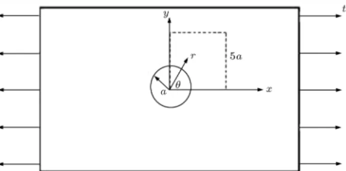
Figure 1. An innite plate with a circular hole under a uniaxial load P.
Figure 2. Boundary conditions of the plate.
ur=4Gt
r
k 1
2 + cos(2)
+ar2
1 + (1 + k) cos(2)
a4
r3 cos(2)
; (40)
u= 4Gt
(1 k)a2 r r
a4
r3
sin(2): (41)
In the above equations, G is the shear modulus and k = (3 v)=(1 + v) with v representing the Poisson's ratio. Due to symmetry, only the upper right square quadrant of the plate is modeled (see Figure 2). The edge length of the square is 5a, with a being the radius of the circular hole. The Dirichlet boundary condition is imposed on the left and bottom boundaries, and the tractions are applied to the top and right edges. The problem is solved under a plane stress conditions. The process begins with the simulation of the problem on two distributions of 95 nodes referred to as initial and rened distributions shown in Figures 3 and 4, respectively. The error distribution is estimated based on the numerical solution obtained using Eq. (14).
After running the CSS algorithm with a uniform distribution of the nodes, the adapted nodes are more
Figure 3. The initial distribution of the nodes.
Figure 4. The rened distribution by the CSS.
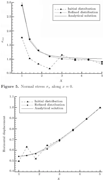
concentrated around the curved edge where the numer-ical errors are much higher due to stress concentration. Comparing the horizontal displacement, ux, of the hole
and the normal stress, x, along x = 0, with analytical
solution of the problem, a tremendous evolution can be seen in the responsiveness of DLSM method by the use of the CSS algorithm, as shown in Figures 5 and 6. Stress tensor for initial solution, the solution of the rened distribution of the nodes by CSS and the real stress tensor for analytical solution are shown in Figure 7.
6.2. A cantilever beam under end load
As a second example, the problem of a cantilever beam under a point load at the end, as shown in Figure 8, is considered. For this problem, the exact stresses and displacements in plane stress are given by Timoshenko and Goodier [24] as:
x= P (L x)yI ; (42)
y = 0; (43)
Figure 5. Normal stress x along x = 0.
Figure 6. The horizontal displacement ux of hole.
Figure 7. Contours of the normal stress x: (a) Initial solution; (b) rened solution; and (c) exact solution.
Figure 8. A cantilever beam under a point load at the end.
Figure 9. Initial nodal distribution.
Figure 10. Rened nodal distribution by the CSS.
Figure 11. The vertical displacement uyalong upper surface of the beam.
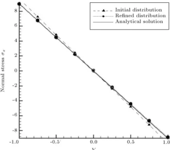
xy= 2IP[c2 y2]; (44)
u = 6EIP y 3x(2L x) + (2 + v)(y2 c2); (45)
v =6EIP y x2(3L x) + 3v(L x)y2+ (4 + 5v)c2x;
(46) where E is the elastic modulus and v represents Poisson's ratio. The moment of inertia I = 2c3=3 is
considered for a beam with rectangular cross-section and unit thickness.
The problem is solved using the DLSM method under plane stress conditions and on the initial con-gurations. A distribution of 125 nodes is used as shown in Figure 9. The errors are calculated and the nodal locations are adaptively altered using the CSS algorithm, as shown in Figure 10. The problem is then resolved on the rened nodal conguration and the results are compared to those obtained on the initial conguration and to the exact analytical results. Figures 11 and 12 compare the vertical displacement,
Figure 12. Normal stress x along upper surface of the beam.
uy, along upper surface of the beam, and the normal
stress x along upper surface of the beam obtained on
the initial and adapted distributions with the analytical solutions. It can be seen that the result obtained on the adapted nodal distribution is virtually exact indicating on the eectiveness of the CSS algorithm in DLSM method.
For large-scale and complex problems the use of meta-heuristic approaches becomes time consuming; however, for such a problem one can decompose it into its components and after solution of each component, the solution of the main problem can be obtained by using the methods provided in Ref. [25].
7. Conclusion
Though the DLSM method has been developed in recent years in order to achieve more accurate solu-tion, renement is inevitable like the other numerical methods. The process of the renement proposed in this paper makes it possible to achieve more accurate responses without increasing the number of points and imposing computational costs. Considering the points in the discretized domain as charged particles in the CSS algorithm and by using the normalized errors in DLSM process as the charges of particles, a powerful model is created. Therefore a node moving in the direction of optimal solution of the problem is obtained. In lectures on adaptivity in meshless methods, dierent techniques are introduced such as that [6] which uses springs between two adjacent nodes, determining the new locations of the nodes requires the solution of a large truss with a computational cost almost as much as time required for solution of the problem. However, since the CSS searches the most suitable locations of the nodes in one or two iteration,
its computational cost is much less than the existing algorithms.
Acknowledgement
The second author is grateful to the Iran National Science Foundation for the support.
References
1. Afshar, M.H. and Arzani, H. \Solving Poissons equa-tions by the discrete least squares meshless method", WIT Transactions on Modeling and Simulation, 42, pp. 23-32 (2004).
2. Firoozjaee, A.R. and Afshar, M.H. \Discrete least squares meshless method with sampling points for the solution of elliptic partial dierential equations", Engineering Analysis with Boundary Elements, 33, pp. 83-92 (2009).
3. Afshar, M.H., Lashckarbolok, M. \Collocated discrete least squares (CDLS) meshless method: Error esti-mate and adaptive renement", International Journal for Numerical Methods in Fluids, 56, pp. 1909-1928 (2008).
4. Naisipour, M., Afshar, M.H., Hassani, B. and Firooz-jaee, A.R. \Collocation discrete least squares (CDLS) method for elasticity problems and grid irregularity eect assessment", American Journal of Applied Sci-ences, 5, pp. 1595-1601 (2008).
5. Afshar, M.H., Amani, J. and Naisipour, M. \A node enrichment adaptive renement in discrete least squares meshless method for solution of elasticity prob-lems", Engineering Analysis with Boundary Elements, 36, pp. 385-393 (2012).
6. Afshar, M.H., Amani, J. and Naisipour, M. \Node moving adaptive renement strategy for planar elas-ticity problems using discrete least squares meshless method", Finite Elements in Analysis and Design, 47, pp. 1315-1325 (2011).
7. Kaveh, A. and Talatahari, S. \A novel heuristic optimization method: Charged system search", Acta Mechanica, 213(3-4), pp. 267-286 (2010).
8. Kaveh, A. and Talatahari, S. \Charged system search for optimal design of frame structures", Applied Soft Computing, 12, pp. 382-393 (2012).
9. Kaveh, A. and Talatahari, S. \Charged system search for optimum grillage systems design using the LRFD-AISC code", Journal of Constructional Steel Research, 66(6), pp. 767-771 (2010).
10. Kaveh, A. and Zolghadr, A. \Truss optimization with natural frequency constraints using a hybridized CSS-BBBC algorithm with trap recognition capability", Computers and Structures, 102-103, pp. 14-27 (2012).
11. Kaveh, A. and Behnam, A.F. \Design optimization of reinforced concrete 3D structures considering fre-quency constraints via a charged system search", Scientia Iranica, 20(3), pp. 387-396 (2013).
12. Kaveh, A. and Shara, P. \Charged system search algorithm for minimax and minisum facility layout problems", Asian Journal of Civil Engineering (Build-ing and Hous(Build-ing), 12(6), pp. 703-718 (2011).
13. Lancaster, P. and Salkauskas, K. \Surfaces generated by moving least squares method", Mathematics of Computation, 37, pp. 141-158 (1981).
14. Onate, E., Perazzo, F. and Miquel, J. \A nite point method for elasticity problems", Computers and Structures, 79, pp. 2151-2163 (2001).
15. Atluri, S.N. The Meshless Local Petrov-Galerkin (MLPG) Method for Domain & Boundary Discretiza-tions, Tech Science Press (2004).
16. Halliday, D., Resnick, R. and Walker, J., Fundamentals of Physics, 8th Ed. John Wiley and Sons (2008).
17. Kaveh, A. and Talatahari, S. \Particle swarm opti-mizer, ant colony strategy and harmony search scheme hybridized for optimization of truss structures", Com-puters and Structures, 87(5-6), pp. 267-283 (2009).
18. Kaveh, A. and Talatahari, S. \A particle swarm ant colony optimization algorithm for truss structures with discrete variables", Journal of Constructional Steel Research, 65(8-9), pp. 1558-1568 (2009).
19. Babuska, I. and Rheinboldt, W.C. \A posteriori error estimates for the nite element method", International Journal for Numerical Methods in Engineering, 12, pp. 1597-1615 (1978).
20. Babuska, I. \The self adaptive approach in the nite element method", in: J.R. White man (Ed.), Mathe-matics of Finite Elements and Applications, Academic Press, London, pp. 125-142 (1975).
21. Zienkiewicz, O.C. and Zhu, J.Z. \The super convergent patch recovery and a posteriori error estimate. Part 1: The recovery technique", International Journal for Numerical Methods in Engineering, 33, pp. 1331-1364 (1995).
22. Zienkiewicz, O.C. and Zhu, J.Z. \The super convergent patch recovery and a posteriori error estimate. Part 2: Error estimate and adaptivity", International Journal for Numerical Methods in Engineering, 33, pp. 1365-1382 (1995).
23. George, P.L. and Borouchaki, H. Delaunay Triangu-lation and Meshing: Application to Finite Elements, HERMES, Paris (1998).
24. Timoshenko, S.P. and Goodier, J.N. Theory of Elas-ticity, 3rd Ed., McGraw-Hill, New York (1987).
25. Kaveh, A. Optimal Analysis of Structures by Concepts of Symmetry and Regularity, Springer Verlag, GmbH, Wien, NewYork (2013).
Biographies
Hamed Arzani was born in 1969 in Amol, Iran. He obtained his BS, MS and PhD degrees in Civil En-gineering, from University of Science and Technology in 1992, 1994, 2006, respectively. He then joined
the University of Shahid Rajaee Teacher Training University in Tehran where he is presently Assistant Professor of Structural Engineering. He is the author of 2 papers published in international journals and 5 papers presented at international conferences.
Ali Kaveh was born in 1948 in Tabriz, Iran. After graduation from the Department of Civil Engineering at the University of Tabriz in 1969, he continued his studies on Structures at Imperial College of Science and Technology at London University, and received his MS, DIC and PhD degrees in 1970 and 1974, respectively. He then joined the Iran University of Science and Technology in Tehran where he is presently Professor of Structural Engineering. Professor Kaveh is the author of 300 papers published in international
journals and 135 papers presented at international conferences. He has authored 23 books in Farsi and 7 books in English published by Wiley, the Ameri-can Mechanical Society, Research Studies Press and Springer.
Mohammad Dehghan was born in 1979 in Doroud, Iran. He obtained his B.S. degree in mathematics at Shahid Chamran University of Ahvaz in 2001, his M.S. degree in mathematical analysis from Lorestan University in 2006, and his second M.S. degree in Structural Engineering from Shahid Rajaee Teacher Training University in 2012. At present, he works on optimum design of dierent structures considering dynamic loadings and irregularities in plan via the meta-heuristic methods.