Decoding by Linear Programming
Emmanuel Candes† and Terence Tao]
† Applied and Computational Mathematics, Caltech, Pasadena, CA 91125 ] Department of Mathematics, University of California, Los Angeles, CA 90095
December 2004
Abstract
This paper considers the classical error correcting problem which is frequently dis-cussed in coding theory. We wish to recover an input vectorf ∈ Rn from corrupted measurementsy=Af+e. Here,Ais anmbyn(coding) matrix andeis an arbitrary and unknown vector of errors. Is it possible to recoverf exactly from the datay?
We prove that under suitable conditions on the coding matrixA, the inputf is the unique solution to the`1-minimization problem (kxk`1:=
P
i|xi|) min
g∈Rn ky−Agk`1
provided that the support of the vector of errors is not too large, kek`0 :=|{i : ei 6=
0}| ≤ρ·m for some ρ >0. In short, f can be recovered exactly by solving a simple convex optimization problem (which one can recast as a linear program). In addition, numerical experiments suggest that this recovery procedure works unreasonably well;
f is recovered exactly even in situations where a significant fraction of the output is corrupted.
This work is related to the problem of finding sparse solutions to vastly underde-termined systems of linear equations. There are also significant connections with the problem of recovering signals from highly incomplete measurements. In fact, the results introduced in this paper improve on our earlier work [5]. Finally, underlying the suc-cess of`1 is a crucial property we call the uniform uncertainty principle that we shall
describe in detail.
Keywords. Linear codes, decoding of (random) linear codes, sparse solutions to
under-determined systems, `1 minimization, basis pursuit, duality in optimization, linear
pro-gramming, restricted orthonormality, principal angles, Gaussian random matrices, singular values of random matrices.
Acknowledgments. E. C. is partially supported by National Science Foundation grants
DMS 01-40698 (FRG) and ACI-0204932 (ITR), and by an Alfred P. Sloan Fellowship. T. T. is supported in part by a grant from the Packard Foundation. Many thanks to Rafail Ostrovsky for pointing out possible connections between our earlier work and the decod-ing problem. E. C. would also like to acknowledge inspirdecod-ing conversations with Leonard Schulmann and Justin Romberg.
1
Introduction
1.1 Decoding of linear codes
This paper considers the model problem of recovering an input vector f ∈ Rn from
cor-rupted measurementsy=Af+e. Here,Ais anmbynmatrix (we will assume throughout
the paper thatm > n), and eis an arbitrary and unknown vector of errors. The problem
we consider is whether it is possible to recoverf exactly from the data y. And if so, how?
In its abstract form, our problem is of course equivalent to the classical error correcting
problem which arises in coding theory as we may think ofAas a linear code; a linear code
is a given collection of codewords which are vectorsa1, . . . , an ∈Rm—the columns of the
matrix A. Given a vector f ∈ Rn (the “plaintext”) we can then generate a vector Af in
Rm (the “ciphertext”); ifAhas full rank, then one can clearly recover the plaintextf from
the ciphertextAf. But now we suppose that the ciphertextAf is corrupted by an arbitrary
vectore∈Rm giving rise to the corrupted ciphertext Af+e. The question is then: given
the coding matrixA and Af +e, can one recoverf exactly?
As is well-known, if the fraction of the corrupted entries is too large, then of course we have
no hope of reconstructing f from Af +e; for instance, assume that m = 2n and consider
two distinct plaintextsf, f0 and form a vectorg∈Rm by setting half of itsm coefficients
equal to those ofAf and half of those equal to those of Af0. Then g=Af +e=Af0+e0
where bothe and e0 are supported on sets of size at mostn=m/2. This simple example
shows that accurate decoding is impossible when the size of the support of the error vector
is greater or equal to a half of that of the outputAf. Therefore, a common assumption in
the literature is to assume that only a small fraction of the entries are actually damaged
kek`0 :=|{i:ei 6= 0}| ≤ρ·m. (1.1)
For which values ofρcan we hope to reconstructewith practical algorithms? That is, with
algorithms whose complexity is at most polynomial in the length mof the code A?
To reconstructf, note that it is obviously sufficient to reconstruct the vectoresince
knowl-edge of Af +e together with e gives Af, and consequently f since A has full rank. Our
approach is then as follows. We construct a matrix which annihilates them×nmatrixA
on the left, i.e. such that F A = 0. This can be done in an obvious fashion by taking a
matrixF whose kernel is the range ofAinRm, which is ann-dimensional subspace (e.g. F
could be the orthogonal projection onto the cokernel ofA). We then applyF to the output
y=Af +eand obtain
˜
y=F(Af +e) =F e (1.2)
since F A = 0. Therefore, the decoding problem is reduced to that of reconstructing a
sparse vectore from the observations F e (by sparse, we mean that only a fraction of the
1.2 Sparse solutions to underdetermined systems
Finding sparse solutions to underdetermined systems of linear equations is in generalN P
-hard [11, 27]. For example, the sparsest solution is given by
(P0) min
d∈Rmkdk`0 subject to F d= ˜y (=F e), (1.3)
and to the best of our knowledge, solving this problem essentially require exhaustive searches
over all subsets of columns ofF, a procedure which clearly is combinatorial in nature and
has exponential complexity.
This computational intractability has recently led researchers to develop alternatives to
(P0), and a frequently discussed approach considers a similar program in the`1-norm which
goes by the name ofBasis Pursuit[8]:
(P1) min
x∈Rmkdk`1, F d= ˜y, (1.4)
where we recall thatkdk`1 =Pm
i=1|di|. Unlike the`0-norm which enumerates the nonzero
coordinates, the `1-norm is convex. It is also well-known [2] that (P1) can be recast as a
linear program (LP).
Motivated by the problem of finding sparse decompositions of special signals in the field of mathematical signal processing and following upon the ground breaking work of Donoho and Huo [13], a series of beautiful articles [14, 15, 21, 30] showed exact equivalence between
the two programs (P0) and (P1). In a nutshell, this work shows that form/2 bymmatrices
F obtained by concatenation of two orthonormal bases, the solution to both (P0) and (P1)
are unique and identical provided that in the most favorable case, the vectorehas at most
.914pm/2 nonzero entries. This is of little practical use here since we are interested in
procedures that might recover a signal when a constant fraction of the output is unreliable. Using very different ideas and together with Romberg [4], the authors proved that the equivalence holds with overwhelming probability for various types of random matrices
pro-vided that propro-vided that the number of nonzero entries in the vector ebe of the order of
m/logm [5, 6]. In the special case whereF is anm/2 by m random matrix with
indepen-dent standard normal entries, [11] proved that the number of nonzero entries may be as
large asρ·m, whereρ >0 is some very small and unspecified positive constant independent
ofm.
1.3 Innovations
This paper introduces the concept of a restrictedly almost orthonormal system—a
collec-tion of vectors which behaves like an almost orthonormal system but only for sparse linear
combinations. Thinking about these vectors as the columns of the matrixF, we show that
this condition allows for the exact reconstruction of sparse linear combination of these
vec-tors, i.e. e. Our results are significantly different than those mentioned above as they are
deterministic and do not involve any kind of randomization, although they can of course be specialized to random matrices. For instance, we shall see that a Gaussian matrix with independent entries sampled from the standard normal distribution is restrictedly
sparse decompositions with a number of nonzero entries of sizeρ0·m; we shall actually give
numerical values for ρ0.
We presented the connection with sparse solutions to underdetermined systems of linear
equations merely for pedagogical reasons. There is a more direct approach. To recover f
from corrupted datay=Af+e, we consider solving the following`1-minimization problem
(P10) min
g∈Rnky−Agk`1. (1.5)
Nowf is the unique solution of (P10) if and only ifeis the unique solution of (P1). In other
words, (P1) and (P10) are equivalent programs. To see why these is true, observe on the one
hand that sincey=Af+e, we may decompose g asg=f +h so that
(P10) ⇔ min
h∈Rnke−Ahk`1.
On the other hand, the constraintF x=F e means that x=e−Ahfor someh∈Rn and,
therefore,
(P1) ⇔ min
h∈Rnkxk`1, x=e−Ah
⇔ min
h∈Rnke−Ahk`1, which proves the claim.
The program (P10) may also be re-expressed as an LP—hence the title of this paper. Indeed,
the`1-minimization problem is equivalent to
min 1Tt, −t≤y−Ag≤t, (1.6)
where the optimization variables are t ∈Rm and g ∈ Rn (as is standard, the generalized
vector inequality x ≤ y means that xi ≤ yi for all i). As a result, (P10) is an LP with
inequality constraints and can be solved efficiently using standard optimization algorithms, see [3].
1.4 Restricted isometries
In the remainder of this paper, it will be convenient to use some linear algebra notations.
We denote by (vj)j∈J ∈ Rp the columns of the matrix F and by H the Hilbert space
spanned by these vectors. Further, for anyT ⊆J, we letFT be the submatrix with column
indicesj ∈T so that
FTc=
X
j∈T
cjvj ∈H.
To introduce the notion of almost orthonormal system, we first observe that if the columns
ofF are sufficiently “degenerate,” the recovery problem cannot be solved. In particular, if
there exists a non-trivial sparse linear combinationP
j∈T cjvj = 0 of thevj which sums to
zero, andT =T1∪T2 is any partition ofT into two disjoint sets, then the vectory
y:= X
j∈T1 cjvj =
X
j∈T2
has two distinct sparse representations. On the other hand, linear dependenciesP
j∈Jcjvj =
0 which involve a large number of nonzero coefficientscj, as opposed to a sparse set of
co-efficients, do not present an obvious obstruction to sparse recovery. At the other extreme,
if the (vj)j∈J are an orthonormal system, then the recovery problem is easily solved by
settingcj =hf, vjiH.
The main result of this paper is that if we impose a “restricted orthonormality hypothesis,”
which is far weaker than assuming orthonormality, then (P1) solves the recovery problem,
even if the (vj)j∈J are highly linearly dependent (for instance, it is possible form:=|J|to
be much larger than the dimension of the span of the vj’s). To make this quantitative we
introduce the following definition.
Definition 1.1 (Restricted isometry constants) Let F be the matrix with the finite
collection of vectors(vj)j∈J ∈Rp as columns. For every integer 1≤S≤ |J|, we define the S-restricted isometry constantsδS to be the smallest quantity such that FT obeys
(1−δS)kck2 ≤ kFTck2 ≤(1 +δS)kck2 (1.7)
for all subsets T ⊂J of cardinality at most S, and all real coefficients (cj)j∈T. Similarly,
we define theS, S0-restricted orthogonality constantsθS,S0 for S+S0≤ |J|to be the smallest quantity such that
|hFTc, FT0c0i| ≤θS,S0 · kck kc0k (1.8)
holds for all disjoint setsT, T0 ⊆J of cardinality |T| ≤S and |T0| ≤S0.
The numbersδSandθSmeasure how close the vectorsvj are to behaving like an orthonormal
system, but only when restricting attention to sparse linear combinations involving no more
thanS vectors. These numbers are clearly non-decreasing in S, S0. ForS = 1, the value
δ1 only conveys magnitude information about the vectorsvj; indeedδ1 is the best constant
such that
1−δ1 ≤ kvjkH2 ≤1 +δ1 for all j∈J. (1.9)
In particular, δ1 = 0 if and only if all of the vj have unit length. Section 2.3 establishes
that the higherδS control the orthogonality numbersθS,S0:
Lemma 1.2 We haveθS,S0 ≤δS+S0 ≤θS,S0+ max(δS, δS0) for allS, S0.
To see the relevance of the restricted isometry numbersδS to the sparse recovery problem,
consider the following simple observation:
Lemma 1.3 Suppose that S ≥1 is such that δ2S < 1, and let T ⊂ J be such that |T| ≤
S. Let f := FT c for some arbitrary |T|-dimensional vector c. Then the set T and the
coefficients (cj)j∈T can be reconstructed uniquely from knowledge of the vector f and the vj’s.
Proof We prove that there is a uniquecwithkck`0 ≤Sand obeyingf =Pjcjvj. Suppose
for contradiction that f had two distinct sparse representations f = FT c = FT0c0 where
|T|,|T0| ≤S. Then
FT∪T0d= 0, dj :=cj1j∈T −cj01j∈T0.
Taking norms of both sides and applying (1.7) and the hypothesisδ2S <1 we conclude that
1.5 Main results
Note that the previous lemma is an abstract existence argument which shows what might
theoretically be possible, but does not supply any efficient algorithm to recoverT and cj
from f and (vj)j∈J other than by brute force search—as discussed earlier. In contrast,
our main theorem result that, by imposing slightly stronger conditions on δ2S, the `1
-minimization program (P1) recovers f exactly.
Theorem 1.4 Suppose that S≥1 is such that
δS+θS+θS,2S <1, (1.10)
and let c be a real vector supported on a set T ⊂J obeying |T| ≤S. Put f :=F c. Then c
is the unique minimizer to
(P1) minkdk`1 F d=f.
Note from Lemma 1.2 that (1.10) impliesδ2S<1, and is in turn implied byδS+δ2S+δ3S <
1/4. Thus the condition (1.10) is roughly “three times as strict” as the condition required
for Lemma 1.3.
Theorem 1.4 is inspired by our previous work [5], see also [4, 6], but unlike those earlier
results, our results here are deterministic, and thus do not have a non-zero probability of
failure, provided of course one can ensure that the system (vj)j∈J verifies the condition
(1.10). By virtue of the previous discussion, we have the companion result:
Theorem 1.5 Suppose F is such that F A = 0 and let S ≥ 1 be a number obeying the
hypothesis of Theorem 1.4. Set y =Af +e, where eis a real vector supported on a set of size at most S. Then f is the unique minimizer to
(P10) min
g∈Rnky−Agk`1.
1.6 Gaussian random matrices
An important question is then to find matrices with good restricted isometry constants,
i.e. such that (1.10) holds for large values ofS. Indeed, such matrices will tolerate a larger
fraction of output in error while still allowing exact recovery of the original input by linear programming. How to construct such matrices might be delicate. In section 3, however, we will argue that generic matrices, namely samples from the Gaussian unitary ensemble
obey (1.10) for relatively large values ofS.
Theorem 1.6 Assume p ≤ m and let F be a p by m matrix whose entries are i.i.d.
Gaussian with mean zero and variance 1/p. Then the condition of Theorem 1.4 holds with overwhelming probability provided that r=S/m is small enough so that
r < r∗(p, m)
where r∗(p, m) is given in Section 3.5. (By “with overwhelming probability,” we mean with probability decaying exponentially inm.) In the limit of large samples,r∗only depends upon the ratio, and numerical evaluations show that the condition holds forr ≤3.6·10−4 in the
In other words, Gaussian matrices are a class of matrices for which one can solve an
un-derdetermined systems of linear equations by minimizing`1 provided, of course, the input
vector has fewer than ρ·m nonzero entries with ρ > 0. We mentioned earlier that this
result is similar to [11] . What is new here is that by using a very different machinery, one can obtain explicit numerical values which were not available before.
In the context of error correcting, the consequence is that a fraction of the output may
be corrupted by arbitrary errors and yet, solving a convex problem would still recover f
exactly—a rather unexpected feat.
Corollary 1.7 Suppose A is an n by m Gaussian matrix and set p =m−n. Under the
hypotheses of Theorem 1.6, the solution to (P10) is unique and equal to f.
This is an immediate consequence of Theorem 1.6. The only thing we need to argue is
why we may think of the annihilator F (such that F A= 0) as a matrix with independent
Gaussian entries. Observe that the range ofAis a random space of dimensionnembedded
inRm so that the data ˜y =F e is the projection of e on a random space of dimension p.
The range of a p by m matrix with independent Gaussian entries precisely is a random
subspace of dimensionp, which justifies the claim.
We would like to point out that the numerical bounds we derived in this paper are overly pessimistic. We are confident that finer arguments and perhaps new ideas will allow to derive versions of Theorem 1.6 with better bounds. The discussion section will enumerate several possibilities for improvement.
1.7 Organization of the paper
The paper is organized as follows. Section 2 proves our main claim, namely, Theorem 1.4 (and hence Theorem 1.5) while Section 3 introduces elements from random matrix theory to establish Theorem 1.6. In Section 4, we present numerical experiments which suggest
that in practice, (P10) works unreasonably well and recovers the f exactly fromy=Af+e
provided that the fraction of the corrupted entries be less than about 17% in the case
wherem= 2n and less than about 34% in the case wherem= 4n. Section 5 explores the
consequences of our results for the recovery of signals from highly incomplete data and ties our findings with some of our earlier work. Finally, we conclude with a short discussion section whose main purpose is to outline areas for improvement.
2
Proof of Main Results
Our main result, namely, Theorem 1.4 is proved by duality. As we will see in section 2.2,c
is the unique minimizer if the matrixFT has full rank and if one can find a vector w with
the two properties
(i) hw, vjiH = sgn(cj) for all j∈T,
where sgn(cj) is the sign of cj (sgn(cj) = 0 forcj = 0). The two conditions above say that
a specific dual program is feasible and is called theexact reconstruction property in [5], see
also [4]. For|T| ≤S withS obeying the hypothesis of Theorem 1.4,FT has full rank since
δS <1 and thus, the proof simply consists in constructing a dual vectorw; this is the object
of the next section.
2.1 Exact reconstruction property
We now examine the sparse reconstruction property and begin with coefficients hw, vjiH
forj6∈T being only small in an`2 sense.
Lemma 2.1 (Dual sparse reconstruction property, `2 version) LetS, S0 ≥1be such
thatδS <1, and cbe a real vector supported onT ⊂J such that|T| ≤S. Then there exists
a vectorw∈H such thathw, vjiH =cj for allj∈T. Furthermore, there is an “exceptional
set” E⊂J which is disjoint from T, of size at most
|E| ≤S0, (2.1)
and with the properties
|hw, vji| ≤
θS,S0
(1−δS)
√
S0 · kck for allj 6∈T∪E
and
(X
j∈E
|hw, vji|2)1/2 ≤ θS
1−δS
· kck.
In addition,kwkH ≤K· kck for some constant K >0 only depending uponδS.
Proof Recall thatFT :`2(T)→H is the linear transformationFT cT :=Pj∈Tcjvj where
cT := (cj)j∈T (we use the subscriptT incT to emphasize that the input is a|T|-dimensional
vector), and letFT∗ be the adjoint transformation
FT∗w:= (hw, vjiH)j∈T.
Property (1.7) gives
1−δS ≤λmin(FT∗FT)≤λmax(FT∗FT)≤1 +δS,
where λmin and λmax are the minimum and maximum eigenvalues of the positive-definite
operatorFT∗FT. In particular, sinceδ|T|<1, we see thatFT∗FT is invertible with
k(FT∗FT)−1k ≤
1
1−δS
. (2.2)
Also note thatkFT(FT∗FT)−1k ≤
√
1 +δS/(1−δS) and setw∈H to be the vector
it is then clear thatFT∗w=cT, i.e. hw, vjiH =cj for allj∈T. In addition,kwk ≤K· kcTk
with K =√1 +δS/(1−δS). Finally, if T0 is any set in J disjoint from T with |T0| ≤ S0
and dT0 = (dj)j∈T0 is any sequence of real numbers, then (1.8) and (2.2) give
|hFT∗0w, dT0i`2(T0)|=|hw, FT0dT0i`2(T0)|= hX
j∈T
((FT∗FT)−1cT)jvj,
X
j∈T0
djvjiH
≤θS,S0 · k(FT∗FT)−1cTk · kdT0k
≤ θS,S0
1−δS
kcTk · kdT0k;
sincedT0 was arbitrary, we thus see from duality that
kFT∗0wk`2(T0)≤
θS,S0
1−δS
kcTk.
In other words,
(X
j∈T0
|hw, vji|2)1/2≤ θS,S0
1−δS
kcTk whenever T0 ⊂J\T and|T0| ≤S0. (2.3)
If in particular if we set
E :={j∈J\T :|hw, vji|>
θS,S0
(1−δS)
√
S0 · kcTk},
then|E|must obey |E| ≤S0, since otherwise we could contradict (2.3) by taking a subset
T0 of E of cardinality S0. The claims now follow.
We now derive a solution with better control on the sup norm of|hw, vji|outside ofT, by
iterating away the exceptional setE (while keeping the values on T fixed).
Lemma 2.2 (Dual sparse reconstruction property, `∞ version) Let S ≥1 be such
thatδS+θS,2S <1, andc be a real vector supported onT ⊂J obeying|T| ≤S. Then there
exists a vector w∈H such that hw, vjiH =cj for allj ∈T. Furthermore, w obeys
|hw, vji| ≤
θS
(1−δS−θS,2S)
√
S · kck for allj6∈T. (2.4)
Proof We may normalize P
j∈T |cj|2 =
√
S. Write T0 := T. Using Lemma 2.1, we can
find a vectorw1 ∈H and a setT1 ⊆J such that
T0∩T1 =∅
|T1| ≤S
hw1, vjiH =cj for all j∈T0
|hw1, vjiH| ≤ θS,S0
(1−δS)
for allj 6∈T0∪T1
(X
j∈T1
|hw1, vjiH|2)1/2 ≤ θS
1−δS
√
S
Applying Lemma 2.1 iteratively gives a sequence of vectorswn+1 ∈ H and sets Tn+1 ⊆J
for alln≥1 with the properties
Tn∩(T0∪Tn+1) =∅
|Tn+1| ≤S
hwn+1, vjiH =hwn, vjiH for all j∈Tn
hwn+1, vjiH = 0 for all j∈T0
|hwn+1, vjiH| ≤ θS
1−δS
θS,2S
1−δS
n
for all j6∈T0∪Tn∪Tn+1
( X
j∈Tn+1
|hwn+1, vji|2)1/2 ≤ θS
1−δS
θS,2S
1−δS
n√
S
kwn+1kH ≤
θS
1−δS
n−1
K.
By hypothesis, we have θS,2S
1−δS ≤1. Thus if we set
w:=
∞
X
n=1
(−1)n−1wn
then the series is absolutely convergent and, therefore,wis a well-defined vector inH. We
now study the coefficients
hw, vjiH = ∞
X
n=1
(−1)n−1hwn, vjiH (2.5)
forj∈J.
Consider firstj∈T0, it follows from the construction thathw1, vjiH =cj andhwn, vjiH = 0
for alln≥2, and hence
hw, vjiH =cj for all j∈T0.
Second, fix j with j 6∈T0 and letIj := {n ≥1 :j ∈Tn}. Since Tn and Tn+1 are disjoint,
we see that the integers in the setIj are spaced at least two apart. Now if n∈Ij, then by
definitionj ∈Tn and, therefore,
hwn+1, vjiH =hwn, vjiH.
In other words, the nand n+ 1 terms in (2.5) cancel each other out. Thus we have
hw, vjiH =
X
n≥1;n,n−16∈Ij
(−1)n−1hwn, vjiH.
On the other hand, ifn, n−16∈Ij and n= 0, then6 j6∈Tn∩Tn−1 and
|hwn, vji| ≤ θS,S
1−δS
θS,2S
1−δS
n−1
which by the triangle inequality and the geometric series formula gives
| X
n≥1;n,n−16∈Ij
(−1)n−1hwn, vjiH| ≤
θS,S
1−δS−θS,2S
In conclusion,
|hw, vjiH −10∈Ijhw0, vjiH| ≤
θS,S
1−δS−θS,2S
,
and since |T| ≤S, the claim follows.
Lemma 2.2 actually solves the dual recovery problem. Indeed, our result states that one
can find a vectorw∈H obeying both properties (i) and (ii) stated at the beginning of the
section. To see why (ii) holds, observe that ksgn(c)k =p|T| ≤ √S and, therefore, (2.4)
gives for all j6∈T
|hw, vjiH| ≤
θS,S
(1−δS−θS,2S)
·
r
|T|
S ≤
θS,S
(1−δS−θS,2S)
<1,
provided thatδS+θS,S+θS,2S <1.
2.2 Proof of Theorem 1.4
Observe first that standard convex arguments give that there exists at least one minimizer
d= (dj)j∈J to the problem (P1). We need to prove thatd=c. Sincecobeys the constraints
of this problem,dobeys
kdk`1 ≤ kck`1 =X
j∈T
|cj|. (2.6)
Now take awobeying properties (i) and (ii) (see the remark following Lemma 2.2). Using
the fact that the inner producthw, vjiis equal to the sign ofcon T and has absolute value
strictly less than one on the complement, we then compute
kdk`1 =X
j∈T
|cj+ (dj−cj)|+
X
j6∈T
|dj|
≥X
j∈T
sgn(cj)(cj + (dj−cj)) +
X
j6∈T
djhw, vjiH
=X
j∈T
|cj|+
X
j∈T
(dj−cj)hw, vjiH +
X
j6∈T
djhw, vjiH
=X
j∈T
|cj|+hw,
X
j∈J
djvj−
X
j∈T cji
=X
j∈T
|cj|+hw, f −fi
=X
j∈T
|cj|.
Comparing this with (2.6) we see that all the inequalities in the above computation must
in fact be equality. Since |hw, vjiH|was strictly less than 1 for all j6∈T, this in particular
forcesdj = 0 for all j /∈T. Thus
X
j∈T
(dj −cj)vj =f −f = 0.
Applying (1.7) (and noting from hypothesis that δS <1) we conclude that dj =cj for all
Remark. It is likely that one may push the conditionδS+θS,S+θS,2S<1 a little further.
The key idea is as follows. Each vector wn in the iteration scheme used to prove Lemma
2.2 was designed to annihilate the influence of wn−1 on the exceptional set Tn−1. But
annihilation is too strong of a goal. It would be just as suitable to designwn to moderate
the influence of wn−1 enough so that the inner product with elements in Tn−1 is small
rather than zero. However, we have not pursued such refinements as the arguments would become considerably more complicated than the calculations presented here.
2.3 Approximate orthogonality
Lemma 1.2 gives control of the size of the principal angle between subspaces of dimension
S and S0 respectively. This is useful because it allows to guarantee exact reconstruction
from the knowledge of theδ numbers only.
Proof [Proof of Lemma 1.2] We first show that θS,S0 ≤ δS+S0. By homogeneity it will
suffice to show that
|hX
j∈T cjvj,
X
j0∈T0
c0j0vj0iH| ≤δS+S0
whenever |T| ≤ S, |T0| ≤ S0, T, T0 are disjoint, and P
j∈T |cj|2 =Pj0∈T0|c0j0|2 = 1. Now
(1.7) gives
2(1−δS+S0)≤ k
X
j∈T cjvj +
X
j0∈T0
c0j0vj0k2
H ≤2(1 +δS+S0)
together with
2(1−δS+S0)≤ k
X
j∈T cjvj−
X
j0∈T0
c0j0vj0k2
H ≤2(1 +δS+S0),
and the claim now follows from the parallelogram identity
hf, gi= kf+gk
2
H − kf −gk2H
4 .
It remains to show thatδS+S0 ≤θS+δS. Again by homogeneity, it suffices to establish that
|hX
j∈T˜ cjvj,
X
j0∈T˜
cj0vj0iH −1| ≤(δS+θS)
whenever |T˜| ≤ S +S0 and P
j∈T˜|cj|2 = 1. To prove this property, we partition ˜T as
˜
T =T∪T0 where|T| ≤S and |T0| ≤S0 and writeP
j∈T |cj|2=αand Pj∈T0|cj|2= 1−α.
(1.7) together with (1.8) give
(1−δS)α≤ h
X
j∈T cjvj,
X
j0∈T
cj0vj0iH ≤(1 +δS)α,
(1−δS0)(1−α)≤ h
X
j∈T0
cjvj,
X
j0∈T0
cj0vj0iH ≤(1 +δS0)(1−α),
|hX
j∈T cjvj,
X
j0∈T
Hence
|hX
j∈T˜ cjvj,
X
j0∈T˜
cj0vj0iH −1| ≤δSα+δS0(1−α) + 2θSα1/2(1−α)1/2
≤max(δS, δS0) +θS
as claimed. (We note that it is possible to optimize this bound a little further but will not do so here.)
3
Gaussian Random Matrices
In this section, we argue that with overwhelming probability, Gaussian random matrices
have “good” isometry constants. Consider a p by m matrix F whose entries are i.i.d.
Gaussian with mean zero and variance 1/p and letT be a subset of the columns. We wish
to study the extremal eigenvalues of FT∗FT. Following upon the work of Marchenko and
Pastur [25], Geman [20] and Silverstein [28] (see also [1]) proved that
λmin(FT∗FT)→(1−
√
γ)2 a.s.
λmax(FT∗FT)→(1 +
√
γ)2 a.s.,
in the limit wherep and |T| → ∞ with
|T|/p→γ ≤1.
In other words, this says that loosely speaking and in the limit of large p, the restricted
isometry constantδ(FT) for a fixedT behaves like
1−δ(FT)≤λmin(FT∗FT)≤λmax(FT)≤1 +δ(FT), δ(FT)≈2
p
|T|/p+|T|/p.
Restricted isometry constants must hold for all setsT of cardinality less or equal toS, and
we shall make use of concentration inequalities to develop such a uniform bound. Note that
forT0⊂T, we obviously have
λmin(FT∗FT)≤λmin(FT∗0FT0)≤λmax(FT∗0FT0)≤λmax(FT∗FT)
and, therefore, attention may be restricted to matrices of sizeS. Now, there are large
devia-tion results about the singular values ofFT [29]. For example, lettingσmax(FT) (resp.σmin)
be the largest singular value of FT so that σmax2 (FT) = λmax(FT∗FT) (resp. σmin2 (FT) =
λmin(FT∗FT)), Ledoux [24] applies the concentration inequality for Gaussian measures, and
for a each fixedt >0, obtains the deviation bounds
P
σmax(FT)>1 +
p
|T|/p+o(1) +t
≤e−pt2/2 (3.1)
P
σmin(FT)<1−
p
|T|/p+o(1)−t
≤e−pt2/2; (3.2)
here,o(1) is a small term tending to zero as p→ ∞and which can be calculated explicitly,
see [16]. For example, this last reference shows that one can selecto(1) in (3.1) as 2p11/3 ·
Lemma 3.1 Put r=S/m and set
f(r) :=pm/p·√r+p2H(r),
where H is the entropy function H(q) :=−qlogq−(1−q) log(1−q) defined for 0< q <1. For each >0, the restricted isometry constant δS of ap by m Gaussian matrix F obeys
P 1 +δS >[1 + (1 +)f(r)]2
≤2·e−mH(r)·/2. (3.3)
Proof As discussed above, we may restrict our attention to sets |T| such that |T| = S.
Denote byηp theo(1)-term appearing in either (3.1) or (3.2). Putλmax=λmax(FT∗FT) for
short, and observe that
P sup
T:|T|=S
λmax>(1 +
p
S/p+ηp+t)2
!
≤ |{T :|T|=S}|Pλmax>(1 +
p
S/p+ηp+t)2
≤ m S
e−pt2/2.
From Stirling’s approximation logm! = mlogm−m+O(logm) we have the well-known
formula log m S
=mH(r) +O(logm).
which gives
P sup
T:|T|=S
λmax>(1 +
p
S/p+ηp+t)2
!
≤emH(r)·eO(logm)·e−pt2/2,
The exact same argument applied to the smallest eigenvalues yields
P
inf
T:|T|=Sλmin<(1
−pS/p−ηp−t)2
≤emH(r)·eO(log(m))·e−pt2/2.
Fixηp+t= (1 +)·
p
m/p·p
2H(r). Assume now that m andp are large enough so that
ηp ≤/2·
p
m/p·p
2H(r). Then
P sup
T:|T|=S
λmax>(1 +
p
S/p+·pm/p·p2H(r))2 !
≤e−mH(r)·/2.
where we used the fact that the termO(logm) is less than mH(r)/2 for sufficiently large
m. The same bound holds for the minimum eigenvalues and the claim follows.
Ignoring the’s, Lemma 3.1 states that with overwhelming probability
δS<−1 + [1 +f(r)]2. (3.4)
A similar conclusion holds forδ2S and δ3S and, therefore, we established that
δS+δ2S+δ3S < ρp/m(r), ρp/m(r) = 3
X
j=1
−1 + [1 +f(jr)]2. (3.5)
with very high probability. In conclusion, Lemma 1.2 shows that the hypothesis of our main
theorem holds provided that the ratio r = S/m be small so that ρp/m(r) < 1. In other
words, in the limit of large samples,S/mmaybe taken as any value obeyingρp/m(S/m)<1
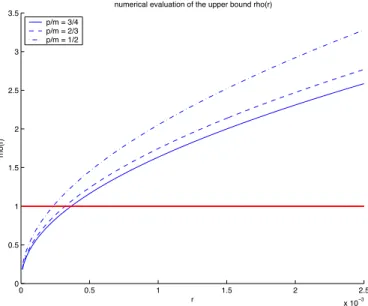
which we used to give numerical values in Theorem 1.6. Figure 1 graphs the functionρp/m(r)
0 0.5 1 1.5 2 2.5 x 10⁻³ 0
0.5 1 1.5 2 2.5 3 3.5
r
rho(r)
numerical evaluation of the upper bound rho(r)
p/m = 3/4 p/m = 2/3 p/m = 1/2
Figure 1: Behavior of the upper bound ρp/m(r) for three values of the ratio p/m, namely,
p/m= 3/4,2/3,1/2.
4
Numerical Experiments
This section investigates the practical ability of `1 to recover an object f ∈ Rn from
corrupted datay =Af +e,y ∈Rm (or equivalently to recover the sparse vector of errors
e∈ Rm from the underdetermined system of equations F e = z ∈ Rm−n). The goal here
is to evaluate empirically the location of the breakpoint as to get an accurate sense of the performance one might expect in practice. In order to do this, we performed a series of experiments designed as follows:
1. selectn(the size of the input signal) andmso that with the same notations as before,
Ais an nby mmatrix; sample Awith independent Gaussian entries;
2. selectS as a percentage ofm;
3. select a support setT of size|T|=S uniformly at random, and sample a vector eon
T with independent and identically distributed Gaussian entries1;
4. make ˜y=Ax+e(the choice ofx does not matter as is clear from the discussion and
here,xis also selected at random), solve (P10) and obtainx∗;
5. comparex tox∗;
6. repeat 100 times for eachS and A;
7. repeat for various sizes ofn andm.
The results are presented in Figure 2 and Figure 3. Figure 2 examines the situation in
which the length of the code is twice that of the input vector m = 2n, for m = 512 and
1Just as in [6], the results presented here do not seem to depend on the actual distribution used to sample
0 0.05 0.1 0.15 0.2 0.25 0.3 0.35 0.4 0.45 0.5 0
0.2 0.4 0.6 0.8 1
# Fraction of corrupted entries
frequency
Empirical frequency of exact reconstruction, n = 256, m = 2n
0 0.05 0.1 0.15 0.2 0.25 0.3 0.35 0.4 0.45 0.5 0
0.2 0.4 0.6 0.8 1
# Fraction of corrupted entries
frequency
Empirical frequency of exact reconstruction, n = 512, m = 2n
(a) (b)
Figure 2: `1-recovery of an input signal fromy=Af+ewithAanmbynmatrix with independent
Gaussian entries. In this experiment, we ’oversample’ the input signal by a factor 2 so thatm= 2n.
(a) Success rate of(P1) form = 512. (b) Success rate of (P1)for m= 1024. Observe the similar
pattern and cut-off point. In these experiments, exact recovery occurs as long as about 17% or less of the entries are corrupted.
m = 1024. Our experiments show that one recovers the input vector all the time as long
as the fraction of the corrupted entries is below 17%. This holds form= 512 (Figure 2(a))
and m = 1024 (Figure 2(b)). In Figure 3, we investigate how these results change as the
length of the codewords increases compared to the length of the input, and examine the
situation in which m = 4n, with m = 512. Our experiments show that one recovers the
input vectorall the time as long as the fraction of the corrupted entries is below 34%.
5
Optimal Signal Recovery
Our recent work [5] developed a set of ideas showing that it is surprisingly possible to reconstruct interesting classes of signals accurately from highly incomplete measurements. The results in this paper are inspired and improve upon this earlier work and we now
elaborate on this connection. Suppose we wish to reconstruct an object α inRm from the
K linear measurements
yk =hα, φki k= 1, . . . , K or y=F α, (5.1)
with φk, the kth row of the matrix F. Of special interest is the vastly underdetermined
case, K << N, where there are many more unknowns than observations. We choose to
formulate the problem abstractly but for concreteness, we might think ofαas the coefficients
α= Ψ∗f of a digital signal or imagef in some nice orthobasis, e.g. a wavelet basis so that
the information about the signal is of the formy=F α=FΨ∗f.
Suppose now that the object of interest is compressible in the sense that the reordered
entries ofα decay like a power-law; concretely, suppose that the entries ofα, rearranged in
decreasing order of magnitude,|α|(1) ≥ |α|(2)≥ · · · ≥ |α|(m), obey
0 0.05 0.1 0.15 0.2 0.25 0.3 0.35 0.4 0.45 0.5 0
0.2 0.4 0.6 0.8 1
# Fraction of corrupted entries
frequency
Empirical frequency of exact reconstruction, n = 128, m = 4n
Figure 3: `1-recovery of an input signal fromy=Af+ewithAanmbynmatrix with independent
Gaussian entries. In this experiment, we ’oversample’ the input signal by a factor 4 so thatm= 4n.
In these experiments, exact recovery occurs as long as about 34% or less of the entries are corrupted.
for somes≥1. We will denote byFs(B) the class of all signalsα∈Rm obeying (5.2). The
claim is that it is possible to reconstruct compressible signals from only a small number of random measurements.
Theorem 5.1 Let F be the measurement matrix as in (5.1) and consider the solutionα]
to
min
˜
α∈Rm kα˜k`1 subject to Fα˜=y. (5.3) Let S≤K such thatδS+ 2θS+θS,2S <1 and set λ=K/S. Then α] obeys
sup
α∈Fs(B)
kα−α]k ≤C·(K/λ)−(s−1/2). (5.4)
To appreciate the content of the theorem, suppose one would have available anoracleletting
us know which coefficients αk, 1 ≤ k ≤ m, are large (e.g. in the scenario we considered
earlier, the oracle would tell us which wavelet coefficients of f are large). Then we would
acquire information about the K largest coefficients and obtain a truncated version αK of
α obeying
kα−αKk ≥c·K−(s−1/2),
for generic elements taken fromFs(B). Now (5.4) says that not knowing anything about
the location of the largest coefficients, one can essentially obtain the same approximation error by nonadaptive sampling, provided the number of measurements be increased by a
factorλ. The largerS, the smaller the oversampling factor, and hence the connection with
the decoding problem. Such considerations make clear that Theorem 5.1 supplies a very concrete methodology for recovering a compressible object from limited measurements and as such, it may have a significant bearing on many fields of science and technology. We refer the reader to [5] and [12] for a discussion of its implications.
Suppose for example thatF is a Gaussian random matrix as in Section 3. We will assume
Calculations identical to those from Section 3 give that with overwhelming probability, F
obeys the hypothesis of the theorem provided that
S≤K/λ, λ=ρ·log(m/K),
for some positive constant ρ > 0. Now consider the statement of the theorem; there is a
way to invoke linear programming and obtain a reconstruction based uponO(Klog(m/K))
measurements only, which is at least as good as that one would achieve by knowing all the
information about f and selecting the K largest coefficients. In fact, this is an optimal
statement as (5.4) correctly identifies the minimum number of measurements needed to
obtain a given precision. In short, it is impossible to obtain a precision of aboutK−(s−1/2)
with fewer thanKlog(m/K) measurements, see [5, 12].
Theorem 5.1 is stronger than our former result, namely, Theorem 1.4 in [5]. To see why this is true, recall the former claim: [5] introduced two conditions, the uniform uncertainty
principle (UUP) and the exact reconstruction principle (ERP). In a nutshell, a random
matrixF obeys the UUP with oversampling factor λifF obeys
δS ≤1/2, S =ρ·K/λ, (5.5)
with probability at least 1−O(N−γ/ρ) for some fixed positive constant γ >0. Second, a
measurement matrixF obeys the ERP with oversampling factor λif for each fixed subset
T of size |T| ≤ S (5.5) and each ‘sign’ vector c defined on T, there exists with the same
overwhelmingly large probability a vector w∈H with the following properties:
(i) hw, vji=cj, for all j∈T;
(ii) and|hw, vji| ≤ 12 for all j not inT.
Note that these are the conditions listed at the beginning of section 2 except for the 1/2
factor on the complement ofT. Fixα∈ Fs(B). [5] argued that if a random matrix obeyed
the UUP and the ERP both with oversampling factorλ, then
kα−α]k ≤C·(K/λ)−(s−1/2),
with inequality holding with the same probability as before. Against this background, several comments are now in order:
• First, the new statement is more general as it applies to all matrices, not just random
matrices.
• Second, whereas our previous statement argued that for each α ∈ Rm, one would
be able—with high probability—to reconstruct α accurately, it did not say anything
about the worst case error for a fixed measurement matrix F. This is an instance
where the order of the quantifiers plays a role. Do we need differentF’s for different
objects? Theorem 5.1 answers this question unambiguously; the sameF will provide
an optimal reconstruction forallthe objects in the class.
• Third, Theorem 5.1 says that the ERP condition is redundant, and hence the
hypoth-esis may be easier to check in practice. In addition, eliminating the ERP isolates the real reason for success as it ties everything down to the UUP. In short, the ability
to recover an object from limited measurements depends on how closeF is to an or-thonormal system, but only when restricting attention to sparse linear combinations of columns.
We will not prove this theorem as this is a minor modification of that of Theorem 1.4 in
the aforementioned reference. The key point is to observe that ifF obeys the hypothesis of
our theorem, then by definition F obeys the UUP with probability one, but F also obeys
the ERP, again with probability one, as this is the content of Lemma 2.2. Hence both the UUP and ERP hold and therefore, the conclusion of Theorem 5.1 follows. (The fact that
the ERP actually holds for all sign vectors of size less thanS is the reason why (5.4) holds
uniformly over all elements taken fromFs(B), see [5].)
6
Discussion
6.1 Connections with other works
In our linear programming model, the plaintext and ciphertext had real-valued components. Another intensively studied model occurs when the plaintext and ciphertext take values
in the finite field F2 := {0,1}. In recent work of Feldman et al. [17], [18], [19], linear
programming methods (based on relaxing the space of codewords to a convex polytope) were developed to establish a polynomial-time decoder which can correct a constant fraction of errors, and also achieve the information-theoretic capacity of the code. There is thus some intriguing parallels between those works and the results in this paper, however there appears to be no direct overlap as our methods are restricted to real-valued texts, and the
work cited above requires texts inF2. Also, our error analysis is deterministic and is thus
guaranteed to correct arbitrary errors provided that they are sufficiently sparse.
The ideas presented in this paper may be adapted to recover input vectors taking values from a finite alphabet. We hope to report on work in progress in a follow-up paper.
6.2 Improvements
There is little doubt that more elaborate arguments will yield versions of Theorem 1.6 with tighter bounds. Immediately following the proof of Lemma 2.2, we already remarked that
one might slightly improve the conditionδS+θS,S+θS,2S <1 at the expense of considerable
complications. More to the point, we must admit that we used well-established tools from Random Matrix Theory and it is likely that more sophisticated ideas might be deployed successfully. We now discuss some of these.
Our main hypothesis readsδS+θS,S+θS,2S<1 but in order to reduce the problem to the
study of those δ numbers (and use known results), our analysis actually relied upon the
more stringent conditionδS+δ2S+δ3S <1 instead, since
δS+θS,S+θS,2S ≤δS+δ2S+δ3S.
This introduces a gap. Consider a fixed setT of size |T|=S. Using the notations of that
Section 3, we argued that
δ(FT)≈2
p
and developed a large deviation bound to quantify the departure from the right hand-side.
Now letT and T0 be two disjoint sets of respective sizes S andS0 and considerθ(FT, FT0):
θ(FT, FT0) is the cosine of the principal angle between the two random subspaces spanned
by the columns ofFT and FT0 respectively; formally
θ(FT, FT0) = suphu, u0i, u∈span(FT), u0 ∈span(FT0),kuk=ku0k= 1.
We remark that this quantity plays an important analysis in statistical analysis because of its use to test the significance of correlations between two sets of measurements, compare
the literature onCanonical Correlation Analysis[26]. Among other things, it is known [31]
that
θ(FT, FT0)→ p
γ(1−γ0) +p
γ0(1−γ) a.s.
as p → ∞ with S/p → γ and S0/p → γ0. In other words, whereas we used the limiting
behaviors
δ(F2T)→2
p
2γ+ 2γ, δ(F3T)→2
p
3γ+ 3γ,
there is a chance one might employ instead
θ(FT, FT0)→2 p
γ(1−γ), θ(FT, FT0)→ p
γ(1−2γ) +p2γ(1−γ)
for|T|=|T0|=S and |T0|= 2|T|= 2S respectively, which is better. Just as in Section 3,
one might then look for concentration inequalities transforming this limiting behavior into corresponding large deviation inequalities. We are aware of very recent work of Johnstone and his colleagues [23] which might be here of substantial help.
Finally, tighter large deviation bounds might exist together with more clever strategies to
derive uniform bounds (valid for allT of size less thanS) from individual bounds (valid for
a singleT). With this in mind, it is interesting to note that our approach hits a limit as
lim inf
S→∞, S/m→r δS+θS,S+θS,2S≥J(m/p·r), (6.1)
whereJ(r) := 2√r+r+ (2 +√2)pr(1−r) +pr(1−2r). SinceJ(r) is greater than 1 if
and only if r >2.36, one would certainly need new ideas to improve Theorem 1.6 beyond
cut-off point in the range of about 2%. The lower limit (6.1) is probably not sharp since it
does not explicitly take into account the ratio betweenm and p; at best, it might serve as
an indication of the limiting behavior when the ration p/mis not too small.
6.3 Other coding matrices
This paper introduced general results stating that it is possible to correct for errors by
`1-minimization. We then explained how the results specialize in the case where the coding
matrix A is sampled from the Gaussian ensemble. It is clear, however, that one could
use other matrices and still obtain similar results; namely, that (P10) recovers f exactly
provided that the number of corrupted entries does not exceed ρ·m. In fact, our previous
work suggests that partial Fourier matrices would enjoy similar properties [5, 6]. Other
candidates might be the so-called noiselets of Coifman, Geshwind and Meyer [9]. These
alternative might be of great practical interest because they would come with fast algorithms
for applying A or A∗ to an arbitrary vector g and, hence, speed up the computations to
References
[1] Z. D. Bai and Y. Q. Yin. Limit of the smallest eigenvalue of a large-dimensional sample
covariance matrix. Ann. Probab. 21(1993), 1275–1294.
[2] P. Bloomfield and W. Steiger. Least Absolute Deviations: Theory, Applications, and
Algorithms. Birkh¨auser, Boston, 1983.
[3] S. Boyd, and L. Vandenberghe, Convex Optimization, Cambridge University Press,
2004.
[4] E. J. Cand`es, J. Romberg, and T. Tao, Robust uncertainty principles: exact signal
re-construction from highly incomplete frequency information. Submitted toIEEE
Trans-actions on Information Theory, June 2004. Available on the ArXiV preprint server:
math.GM/0409186.
[5] E. J. Cand`es, and T. Tao, Near optimal signal recovery from random projections:
uni-versal encoding strategies? Submitted to IEEE Transactions on Information Theory,
October 2004. Available on the ArXiV preprint server: math.CA/0410542.
[6] E. J. Cand`es, and J. Romberg, Quantitative Robust Uncertainty Principles and
Op-timally Sparse Decompositions. Submitted to Foundations of Computational
Mathe-matics, November 2004. Available on the ArXiV preprint server: math.CA/0411273. [7] S. S. Chen. Basis Pursuit. Stanford Ph. D. Thesis, 1995.
[8] S. S. Chen, D. L. Donoho, and M. A. Saunders. Atomic decomposition by basis pursuit. SIAM J. Scientific Computing 20(1999), 33–61.
[9] R. Coifman, F. Geshwind, and Y. Meyer. Noiselets.Appl. Comput. Harmon. Anal. 10
(2001), 27–44.
[10] K. R. Davidson and S. J. Szarek. Local operator theory, random matrices and Banach
spaces. In: Handbook in Banach Spaces Vol I, ed. W. B. Johnson, J. Lindenstrauss,
Elsevier (2001), 317–366.
[11] D. L. Donoho. For Most Large Underdetermined Systems of Linear Equations the
Minimal`1-norm Solution is also the Sparsest Solution. Manuscript, September 2004.
[12] D. L. Donoho, Compressed Sensing, Manuscript, September 2004.
[13] D. L. Donoho and X. Huo. Uncertainty principles and ideal atomic decomposition. IEEE Transactions on Information Theory,47(2001), 2845–2862.
[14] D. L. Donoho and M. Elad. Optimally sparse representation in general (nonorthogonal)
dictionaries via `1 minimization, Proc. Natl. Acad. Sci. USA100 (2003), 2197–2202.
[15] M. Elad and A. M. Bruckstein. A generalized uncertainty principle and sparse
repre-sentation in pairs ofRN bases.IEEE Transactions on Information Theory,48(2002),
2558–2567.
[16] N. El Karoui. New Results about Random Covariance Matrices and Statistical Appli-cations. Stanford Ph. .D. Thesis, August 2004.
[17] J. Feldman. Decoding Error-Correcting Codes via Linear Programming. Ph.D. Thesis 2003, Massachussets Institute of Technology.
[18] J. Feldman. LP decoding achieves capacity, 2005 ACM-SIAM Symposium on Discrete Algorithms (SODA), preprint (2005).
[19] J. Feldman, T. Malkin, C. Stein, R. A. Servedio, M. J. Wainwright. LP Decoding
Corrects a Constant Fraction of Errors. Proc. IEEE International Symposium on
In-formation Theory (ISIT), June 2004.
[20] S. Geman. A limit theorem for the norm of random matrices. Ann. Probab. 8 (1980),
252–261.
[21] R. Gribonval and M. Nielsen. Sparse representations in unions of bases.IEEE Trans.
Inform. Theory 49(2003), 3320–3325.
[22] I. M. Johnstone. On the distribution of the largest eigenvalue in principal components
analysis.Ann. Statist.29 (2001), 295–327.
[23] I. M. Johnstone. Large covariance matrices. Third 2004 Wald Lecture, 6th World Congress of the Bernoulli Society and 67th Annual Meeting of the IMS, Barcelona, July 2004.
[24] M. Ledoux. The concentration of measure phenomenon. Mathematical Surveys and
Monographs 89, American Mathematical Society, Providence, RI, 2001.
[25] V. A. Marchenko and L. A. Pastur. Distribution of eigenvalues in certain sets of random
matrices.Mat. Sb. (N.S.) 72(1967), 407–535 (in Russian).
[26] R. J. Muirhead.Aspects of multivariate statistical theory. Wiley Series in Probability
and Mathematical Statistics. John Wiley & Sons, Inc., New York, 1982.
[27] B. K. Natarajan. Sparse approximate solutions to linear systems. SIAM J. Comput.
24 (1995), 227-234.
[28] J. W. Silverstein. The smallest eigenvalue of a large dimensional Wishart matrix.Ann.
Probab. 13(1985), 1364–1368.
[29] S. J. Szarek. Condition numbers of random matrices.J. Complexity7(1991), 131–149.
[30] J. A. Tropp. Greed is good: Algorithmic results for sparse approximation. Technical Report, The University of Texas at Austin, 2003.
[31] K. W. Wachter. The limiting empirical measure of multiple discriminant ratios. Ann.