Probability Estimates for Multi-class Classification by Pairwise Coupling

(1)

Probability Estimates for Multi-class Classification by

Pairwise Coupling

Ting-Fan Wu [email protected]

Chih-Jen Lin [email protected]

Department of Computer Science National Taiwan University Taipei 106, Taiwan

Ruby C. Weng [email protected]

Department of Statistics National Chengchi University Taipei 116, Taiwan

Editor: Yoram Singer

Abstract

Pairwise coupling is a popular multi-class classification method that combines all com-parisons for each pair of classes. This paper presents two approaches for obtaining class probabilities. Both methods can be reduced to linear systems and are easy to implement. We show conceptually and experimentally that the proposed approaches are more stable than the two existing popular methods: voting and the method by Hastie and Tibshirani (1998).

Keywords: Pairwise Coupling, Probability Estimates, Random Forest, Support Vector Machines

1. Introduction

The multi-class classification problem refers to assigning each of the observations into one of k classes. As two-class problems are much easier to solve, many authors propose to use two-class classifiers for multi-class classification. In this paper we focus on techniques that provide a multi-class probability estimate by combining all pairwise comparisons.

A common way to combine pairwise comparisons is by voting (Knerr et al., 1990; Fried-man, 1996). It constructs a rule for discriminating between every pair of classes and then selecting the class with the most winning two-class decisions. Though the voting procedure requires just pairwise decisions, it only predicts a class label. In many scenarios, however, probability estimates are desired. As numerous (pairwise) classifiers do provide class proba-bilities, several authors (Refregier and Vallet, 1991; Price et al., 1995; Hastie and Tibshirani, 1998) have proposed probability estimates by combining the pairwise class probabilities.

Given the observation x and the class label y, we assume that the estimated pairwise class probabilities rij of µij =P(y =i|y =iorj,x) are available. From the ith and jth classes of a training set, we obtain a model which, for any newx, calculatesrij as an approx-imation ofµij. Then, using allrij, the goal is to estimate pi =P(y=i|x), i= 1, . . . , k. In this paper, we first propose a method for obtaining probability estimates via an

(2)

approxima-tion soluapproxima-tion to an identity. The existence of the soluapproxima-tion is guaranteed by theory in finite Markov Chains. Motivated by the optimization formulation of this method, we propose a second approach. Interestingly, it can also be regarded as an improved version of the cou-pling approach given by Refregier and Vallet (1991). Both of the proposed methods can be reduced to solving linear systems and are simple in practical implementation. Furthermore, from conceptual and experimental points of view, we show that the two proposed methods are more stable than voting and the method by Hastie and Tibshirani (1998).

We organize the paper as follows. In Section 2, we review several existing methods. Sections 3 and 4 detail the two proposed approaches. Section 5 presents the relationship between different methods through their corresponding optimization formulas. In Section 6, we compare these methods using simulated data. In Section 7, we conduct experiments using real data. The classifiers considered are support vector machines and random forest. A preliminary version of this paper was presented in (Wu et al., 2004).

2. Survey of Existing Methods

For methods surveyed in this section and those proposed later, each provides a vector of multi-class probability estimates. We denote it as p∗ according to method _∗. Similarly, there is an associated rule arg maxi[p∗i] for prediction and we denote the rule as δ∗.

2.1 Voting

Let rij be the estimates of µij ≡ P(y = i | y = ior j,x) and assume rij +rji = 1. The voting rule (Knerr et al., 1990; Friedman, 1996) is

δV = arg max i [

X

j:j6=i

I_{rij>rji}], (1)

whereI is the indicator function: I_{x_}= 1 ifxis true, and 0 otherwise. A simple estimate of probabilities can be derived as

pv_i = 2 X j:j6=i

I{rij>rji}/(k(k−1)).

2.2 Method by Refregier and Vallet

Withµij =pi/(pi+pj), Refregier and Vallet (1991) consider that

rij

rji ≈

µij

µji = pi

pj

. (2)

Thus, making (2) an equality may be a way to solvepi. However, the number of equations,

k(k₋1)/2, is more than the number of unknownsk, so Refregier and Vallet (1991) propose to choose any k₋1 rij. Then, with the condition Pk_i=1pi = 1, pRV can be obtained by solving a linear system. However, as pointed out previously by Price et al. (1995), the results depend strongly on the selection ofk₋1 rij.

In Section 4, by considering (2) as well, we propose a method which remedies this problem.

(3)

2.3 Method by Price, Kner, Personnaz, and Dreyfus Price et al. (1995) consider that



 X

j:j6=i

P(y=iorj_|x) 

−(k−2)P(y=i|x) =

k

X

j=1

P(y =j_|x) = 1.

Using

rij ≈µij =

P(y=i_|x)

P(y=ior j_|x), one obtains

pP KP D_i = _P 1

j:j6=ir1ij −(k−2)

. (3)

As Pk

i=1pi = 1 does not hold, we must normalize pP KP D. This approach is very simple and easy to implement. In the rest of this paper, we refer to this method as PKPD. 2.4 Method by Hastie and Tibshirani

Hastie and Tibshirani (1998) propose to minimize the Kullback-Leibler (KL) distance be-tweenrij and µij:

l(p) = X i6=j

nijrijlog

rij

µij

, (4)

= X

i<j

nij

rijlog

rij

µij

+ (1₋rij) log

1₋rij 1₋µij

,

whereµij =pi/(pi+pj),rji= 1−rij, andnij is the number of training data in the ith and

jth classes.

To minimize (4), they first calculate

∂l(p)

∂pi

= X

j:j6=i

nij −

rij

pi

+ 1

pi+pj

.

Thus, letting ∂l(p)/∂pi = 0, i = 1, . . . , k and multiplying pi on each term, Hastie and Tibshirani (1998) propose finding a point that satisfies

X

j:j6=i

nijµij =

X

j:j6=i

nijrij,

k

X

i=1

pi= 1,and pi >0, i= 1, . . . , k. (5)

Such a point is obtained by the following algorithm: Algorithm 1

(4)

2. Repeat(i= 1, . . . , k,1, . . .)

α= P

j:j6=inijrij

P

j:j6=inijµij

(6)

µij ←

αµij

αµij +µji

, µji←1−µij, for all j6=i (7)

pi ←αpi (8)

normalizep(optional) (9)

until kconsecutive α are all close to ones. 3. p_←p/Pk

i=1pi

(8) implies that in each iteration, only theith component is updated and all others remain the same. There are several remarks about this algorithm. First, the initial p must be positive so that all later p are positive and α is well defined (i.e., no zero denominator in (6)). Second, (9) is an optional operation because whether we normalize p or not does not affect the values of µij and α in (6) and (7).

Hastie and Tibshirani (1998) prove that Algorithm 1 generates a sequence of points at which the KL distance is strictly decreasing. However, Hunter (2004) indicates that the strict decrease in l(p) does not guarantee that any limit point satisfies (5). Hunter (2004) discusses the convergence of algorithms for generalized Bradley-Terry models where Algorithm 1 is a special case. It points out that Zermelo (1929) has proved that, if rij > 0,_∀i₆= j, for any initial point, the whole sequence generated by Algorithm 1 converges to a point satisfying (5). Furthermore, this point is the unique global minimum ofl(p) under the constraints Pk

i=1pi = 1 and 0≤pi≤1, i= 1, . . . , k.

LetpHT denote the global minimum ofl(p). It is shown in Zermelo (1929) and Theorem 1 of (Hastie and Tibshirani, 1998) that if weights nij in (4) are considered equal, thenpHT satisfies

pHT_i > pHT_j if and only if ˜pHT_i _≡ 2 P

s:i6=sris

k(k₋1) >p˜ HT j ≡

2P

s:j6=srjs

k(k₋1) . (10) Therefore, ˜pHT _{is sufficient if one only requires the classification rule. In fact, ˜}_pHT _{can be} derived as an approximation to the identity

pi=

X

j:j6=i

pi+pj

k₋1

pi

pi+pj

= X

j:j6=i

pi+pj

k₋1

µij (11)

by replacingpi+pj with 2/k, andµij withrij in (11). We refer to the decision rule asδHT, which is essentially

arg max i [˜p

HT

i ]. (12)

In the next two sections, we propose two methods which are simpler in both practical implementation and algorithmic analysis.

If the multi-class data are balanced, it is reasonable to assume equal weighting (i.e.,

nij = 1) as the above. In the rest of this paper, we restrict our discussion under such an assumption.

(5)

3. Our First Approach

As δHT relies on pi+pj ≈ 2/k, in Section 6 we use two examples to illustrate possible problems with this rule. In this section, instead of replacing pi +pj by 2/k in (11), we propose to solve the system:

pi =

X

j:j6=i

(pi+pj

k₋1 )rij,∀i, subject to k

X

i=1

pi= 1, pi ≥0,∀i. (13) Letp1 _{denote the solution to (13). Then the resulting decision rule is}

δ1= arg max i [p

1 i]. 3.1 Solving (13)

To solve (13), we rewrite it as

Qp=p,

k

X

i=1

pi = 1, pi≥0,∀i, whereQij ≡

(

rij/(k−1) ifi6=j,

P

s:s6=iris/(k−1) ifi=j.

(14) Observe that Pk

i=1Qij = 1 for j = 1, . . . , k and 0 ≤ Qij ≤ 1 for i, j = 1, . . . , k, so there exists a finite Markov Chain whose transition matrix is Q. Moreover, if rij > 0 for all

i ₆= j, then Qij > 0, which implies that this Markov Chain is irreducible and aperiodic. From Theorem 4.3.3 of Ross (1996), these conditions guarantee the existence of a unique stationary probability and all states being positive recurrent. Hence, we have the following theorem:

Theorem 1 If rij >0, i6=j, then (14) has a unique solution p with0< pi <1 ∀i. Assume the solution from Theorem 1 is p∗_{. We claim that without the constraints}

pi ≥0,∀i, the linear system

Qp=p,

k

X

i=1

pi= 1 (15)

still has the same unique solution p∗. Otherwise, there is another solution ¯p∗(₆=p∗). Then for any 0_≤λ_≤1,λp∗+ (1₋λ)¯p∗ satisfies (15) as well. Asp∗_i >0,_∀i, whenλis sufficiently close to 1,λp∗

i+(1−λ)¯p∗i >0, i= 1, . . . , k.This violates the uniqueness property in Theorem 1.

Therefore, unlike the method in Section 2.4 where a special iterative procedure has to be implemented, here we only solve a simple linear system. As (15) has k+ 1 equalities but only k variables, practically we remove any one equality from Qp = p and obtain a square system. Since the column sum of Q is the vector of all ones, the removed equality is a linear combination of all remaining equalities. Thus, any solution of the square system satisfies (15) and vice versa. Therefore, this square system has the same unique solution as (15) and hence can be solved by standard Gaussian elimination.

Instead of Gaussian elimination, as the stationary solution of a Markov Chain can be derived by the limit of the n-step transition probability matrix Qn, we can solve (13) by repeatedly multiplyingQ with any initial probability vector.

(6)

3.2 Another Look at (13)

The following arguments show that the solution to (13) is a global minimum of a meaningful optimization problem. To begin, using the property thatrij+rji= 1,∀i6=j, we re-express

pi =P_j:j₆_=i(p_ki+p₋₁j)rij of (14) (i.e.,Qp =p of (15)) as

X

j:j6=i

rjipi−

X

j:j6=i

rijpj = 0, i= 1, . . . , k.

Therefore, a solution of (14) is in fact the unique global minimum of the following convex problem:

min

p

k

X

i=1 (X

j:j6=i

rjipi−

X

j:j6=i

rijpj)2

subject to k

X

i=1

pi = 1, pi≥0, i= 1, . . . , k. (16) The reason is that the object function is always nonnegative, and it attains zero under (14). Note that the constraintspi ≥0∀iare not redundant following the discussion around Equation (15).

4. Our Second Approach

Note that both approaches in Sections 2.4 and 3 involve solving optimization problems using relations likepi/(pi+pj)≈rij orP_j:j₆_=irjipi≈P_j:j₆_=irijpj. Motivated by (16), we suggest another optimization formulation as follows:

min

p

k

X

i=1

X

j:j6=i

(rjipi−rijpj)2 subject to k

X

i=1

pi = 1, pi ≥0,∀i. (17) Note that the method (Refregier and Vallet, 1991) described in Section 2.2 considers a random selection ofk₋1 equations of the formrjipi =rijpj. As (17) considers all rijpj−

rjipi, not just k−1 of them, it can be viewed as an improved version of the coupling approach by Refregier and Vallet (1991).

Let p2 denote the corresponding solution. We then define the classification rule as

δ2= arg max i [p

2 i]. 4.1 A Linear System from (17)

Since (16) has a unique solution, which can be obtained by solving a simple linear system, it is desirable to see whether the minimization problem (17) has these nice properties. In this subsection, we show that (17) has a unique solution and can be solved by a simple linear system.

First, the following theorem shows that the nonnegative constraints in (17) are redun-dant.

(7)

Theorem 2 Problem (17) is equivalent to

min

p

k

X

i=1

X

j:j6=i

(rjipi−rijpj)2 subject to k

X

i=1

pi= 1. (18)

The proof is in Appendix A. Note that we can rewrite the objective function of (18) as min

p 2p

T

Qp_≡min

p

1 2p

T

Qp, (19)

where

Qij =

( P

s:s6=irsi2 ifi=j,

−rjirij ifi6=j.

(20) We divide the objective function by a positive factor of four so its derivative is a simple form

Qp. From (20),Qis positive semi-definite as for anyv₆=0,vTQv= 1/2Pk

i=1

Pk

j=1(rjivi−

rijvj)2 ≥0. Therefore, without constraints pi ≥0,∀i, (19) is a linear-equality-constrained convex quadratic programming problem. Consequently, a point p is a global minimum if and only if it satisfies the optimality condition: There is a scalar bsuch that

Q e

eT ₀ p

b

=

0 1

. (21)

Here Qp is the derivative of (19), bis the Lagrangian multiplier of the equality constraint Pk

i=1pi = 1, eis the k×1 vector of all ones, and 0 is the k×1 vector of all zeros. Thus, the solution to (17) can be obtained by solving the simple linear system (21).

4.2 Solving (21)

Equation (21) can be solved by some direct methods in numerical linear algebra. Theorem 3(i) below shows that the matrix in (21) is invertible; therefore, Gaussian elimination can be easily applied.

For symmetric positive definite systems, Cholesky factorization reduces the time for Gaussian elimination by half. Though (21) is symmetric but not positive definite, if Q is positive definite, Cholesky factorization can be used to obtain b=₋1/(eT_Q−1_e_{) first and} then p = ₋bQ−1_e_{. Theorem 3(ii) shows that} _Q _{is positive definite under quite general} conditions. Moreover, even if Q is only positive semi-definite, Theorem 3(i) proves that

Q+ ∆eeT _{is positive definite for any constant ∆} _> _{0. Along with the fact that (21) is} equivalent to

Q+ ∆eeT _e

eT 0

p

b

=

∆e 1

,

we can do Cholesky factorization on Q+ ∆eeT _{and solve} _b _and _p _{similarly, regardless} whether Qis positive definite or not.

(8)

(i) For any ∆>0, Q+ ∆eeT _{is positive definite. In addition,} hQ e eT 0 i

is invertible, and hence (17) has a unique global minimum.

(ii) If for any i= 1, . . . , k, there are s₆=j for which s₆=i, j ₆=i, and

rsirjs

ris 6

= rjirsj

rij

, (22)

then Q is positive definite.

We leave the proof in Appendix B.

In addition to direct methods, next we propose a simple iterative method for solving (21):

Algorithm 2

1. Start with some initialpi≥0,∀iand Pk_i=1pi= 1. 2. Repeat(t= 1, . . . , k,1, . . .)

pt← 1

Qtt [₋X

j:j6=t

Qtjpj+pTQp] (23)

normalizep (24)

until (21) is satisfied.

Equation (20) and the assumptionrij >0,∀i6=j, ensure that the right-hand side of (23) is always nonnegative. For (24) to be well defined, we must ensure thatPk

i=1pi>0 after the operation in (23). This property holds (see (40) for more explanation). With b=₋pT_Q_p obtained from (21), (23) is motivated from the tth equality in (21) with b replaced by

−pT_Q_p_{. The convergence of Algorithm 2 is established in the following theorem:}

Theorem 4 If rsj > 0,∀s =6 j, then {pi}∞i=1, the sequence generated by Algorithm 2,

converges globally to the unique minimum of (17).

The proof is in Appendix C. Algorithm 2 is implemented in the software LIBSVM

developed by Chang and Lin (2001) for multi-class probability estimates. We discuss some implementation issues of Algorithm 2 in Appendix D.

5. Relations Between Different Methods

Among the methods discussed in this paper, the four decision rulesδHT,δ1,δ2, andδV can be written as arg maxi[pi], wherepis derived by the following four optimization formulations

(9)

under the constraints Pk

i=1pi= 1 and pi ≥0,∀i:

δHT : min

p

k

X

i=1 [X

j:j6=i (rij

1

k −

1 2pi)]

2_, ₍₂₅₎

δ1 : min

p

k

X

i=1 [X

j:j6=i

(rijpj−rjipi)]2, (26)

δ2 : min

p

k

X

i=1

X

j:j6=i

(rijpj−rjipi)2, (27)

δV : min

p

k

X

i=1

X

j:j6=i

(I{rij>rji}pj −I{rji>rij}pi)

2_. ₍₂₈₎

Note that (25) can be easily verified from (10), and that (26) and (27) have been explained in Sections 3 and 4. For (28), its solution is

pi=

c P

j:j6=iI{rji>rij}

, (29)

wherecis the normalizing constant; and therefore, arg maxi[pi] is the same as (1).1 Detailed derivation of (29) is in Appendix E.

Clearly, (25) can be obtained from (26) by letting pj = 1/k and rji = 1/2. Such approximations ignore the differences betweenpi. Next, (28) is from (27) withrij replaced by I_{rij>rji}, and hence, (28) may enlarge the differences betweenpi. Moreover, compared

with (27), (26) allows the difference betweenrijpj andrjipi to be canceled first, so (26) may tend to underestimate the differences betweenpi. In conclusion, conceptually, (25) and (28) are more extreme – the former tends to underestimate the differences betweenpi, while the latter overestimates them. These arguments will be supported by simulated and real data in the next two sections.

For PKPD approach (3), the decision rule can be written as:

δP KP D= arg min i [

X

j:j6=i 1

rij ].

This form looks similar to δHT = arg maxi[P_j:j₆_=irij], which can be obtained from (10) and (12). Notice that the differences amongP

j:j6=irij tend to be larger than those among

P

j:j6=ir1ij, because 1/rij > 1 > rij. More discussion on these two rules will be given in

Section 6.

6. Experiments on Synthetic Data

In this section, we use synthetic data to compare the performance of existing methods described in Section 2 as well as two new approaches proposed in Sections 3 and 4. Here we 1. ForI{r_ij>r_ji}to be well defined, we considerrij6=rji, which is generally true. In addition, if there is an

ifor whichP

j:j6=iI{rji>rij}= 0, an optimal solution of (28) ispi= 1, andpj= 0,∀j6=i. The resulting decision is the same as that of (1).

(10)

do not include the method in Section 2.2 because its results depend strongly on the choice of k₋1rij and our second method is an improved version of it.

Hastie and Tibshirani (1998) design a simple experiment in which all pi are fairly close and their method δHT outperforms the voting strategy δV. We conduct this experiment first to assess the performance of our proposed methods. Following their settings, we define class probabilities

(a) p1 = 1.5/k,pj = (1−p1)/(k−1),j= 2, . . . , k, and then set

rij =

pi

pi+pj

+ 0.1zij ifi > j, (30)

rji=

pj

pi+pj

+ 0.1zji = 1−rij ifj > i, (31) where zij are standard normal variates andzji =−zij. Sincerij are required to be within (0,1), we truncate rij at ǫ below and 1−ǫabove, with ǫ= 10−7. In this example, class 1 has the highest probability and hence is the correct class.

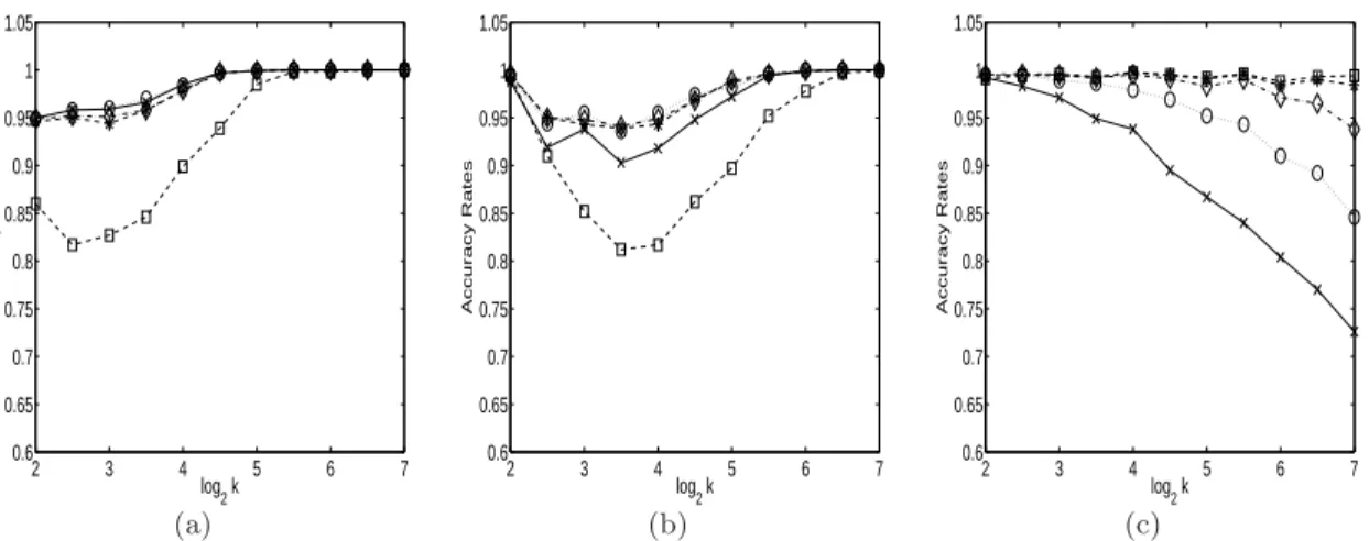
Figure 2(a) shows accuracy rates for each of the five methods when k = 22,_⌈22.5_⌉,

23_{, . . . ,}₂7_{, where} _⌈_x_⌉ _{denotes the largest integer not exceeding} _x_{. The accuracy rates are} averaged over 1,000 replicates. Note that in this experiment all classes are quite competitive, so, when using δV, sometimes the highest vote occurs at two or more different classes. We handle this problem by randomly selecting one class from the ties. This partly explains the poor performance of δV. Another explanation is that the rij here are all close to 1/2, but (28) uses 1 or 0 instead, as stated in the previous section; therefore, the solution may be severely biased. Besides δV, the other four rules have good performance in this example.

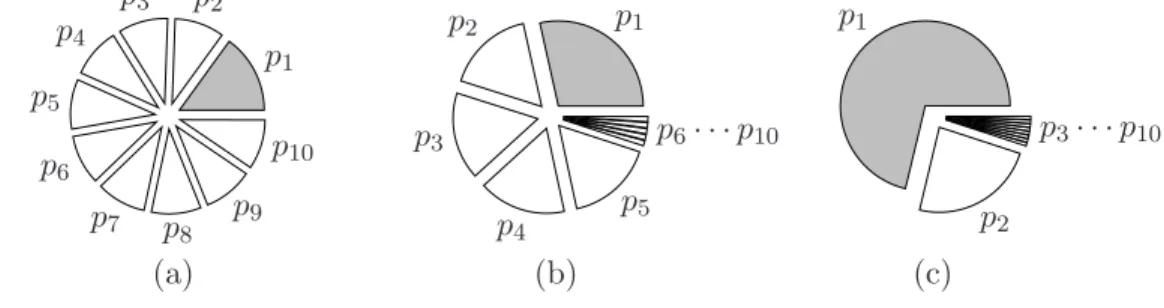
Since δHT relies on the approximation pi +pj ≈ k/2, this rule may suffer some losses if the class probabilities are not highly balanced. To examine this point, we consider the following two sets of class probabilities:

(b) We letk1 =k/2 ifkis even, and (k+1)/2 ifkis odd; then we definep1 = 0.95×1.5/k1,

pi = (0.95−p1)/(k1−1) fori= 2, . . . , k1, andpi = 0.05/(k−k1) fori=k1+ 1, . . . , k. (c) We definep1= 0.95×1.5/2, p2 = 0.95−p1, and pi= 0.05/(k−2), i= 3, . . . , k. An illustration of these three sets of class probabilities is in Figure 1.

p1

p2

p3

p4

p5

p6

p7 _p₈ p9

p10

p1

p2

p3

p4

p5

p6· · ·p10

p1

p2

p3· · ·p10

(a) (b) (c)

(11)

After settingpi, we define the pairwise comparisonsrij as in (30)-(31). Both experiments are repeated for 1,000 times. The accuracy rates are shown in Figures 2(b) and 2(c). In both scenarios, pi are not balanced. As expected,δHT is quite sensitive to the imbalance of

pi. The situation is much worse in Figure 2(c) because the approximation pi+pj ≈k/2 is more seriously violated, especially whenk is large.

A further analysis of Figure 2(c) shows that when kis large,

r12= 3

4+ 0.1z12, r1j ≈1 + 0.1z1j, j≥3,

r21= 1

4+ 0.1z21, r2j ≈1 + 0.1z2j, j≥3,

rij ≈0 + 0.1zij, i6=j, i≥3,

wherezji=−zij are standard normal variates. From (10), the decision ruleδHT in this case is mainly on comparing P

j:j6=1r1j and

P

j:j6=2r2j. The difference between these two sums is 1₂ + 0.1(P

j:j6=1z1j −Pj:j6=2z2j), where the second term has zero mean and, when k is large, high variance. Therefore, for largek, the decision depends strongly on these normal variates, and the probability of choosing the first class is approaching half. On the other hand,δP KP D relies on comparing

P

j:j6=11/r1j andPj:j6=21/r2j. As the difference between 1/r12 and 1/r21 is larger than that between r12 and r21, though the accuracy rates decline when kincreases, the situation is less serious.

We also analyze the mean square error (MSE) in Figure 3:

MSE = 1

1000 1000

X

j=1 1

k

X

i=1

(ˆpj_i ₋pi)2, (32)

where ˆpj_{is the probability estimate obtained in the}_j_{th of the 1,000 replicates. Overall,}_δ HT and δV have higher MSE, confirming again that they are less stable. Note that Algorithm 1 and (10) give the same prediction forδHT, but their MSE are different. Here we consider (10) as it is the one analyzed and compared in Section 5.

In summary, δ1 and δ2 are less sensitive to pi, and their overall performance are fairly stable. All observations aboutδHT,δ1,δ2, andδV here agree with our analysis in Section 5. Despite some similarity toδHT,δP KP D outperformsδHT in general. Experiments in this study are conducted using MATLAB.

7. Experiments on Real Data

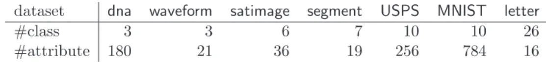
In this section we present experimental results on several multi-class problems: dna, satim-age, segment, and letter from the Statlog collection (Michie et al., 1994), waveform from UCI Machine Learning Repository (Blake and Merz, 1998),USPS(Hull, 1994), andMNIST

(LeCun et al., 1998). The numbers of classes and features are reported in Table 7. Ex-cept dna, which takes two possible values 0 and 1, each attribute of all other data is linearly scaled to [₋1,1]. In each scaled data, we randomly select 300 training and 500 testing instances from thousands of data points. 20 such selections are generated and the testing error rates are averaged. Similarly, we do experiments on larger sets (800 training and 1,000 testing). All training and testing sets used are available at http://

(12)

2 3 4 5 6 7 0.6 0.65 0.7 0.75 0.8 0.85 0.9 0.95 1 1.05 log

2 k

Accuracy Rates

(a)

2 3 4 5 6 7

0.6 0.65 0.7 0.75 0.8 0.85 0.9 0.95 1 1.05 log

2 k

Accuracy Rates

(b)

2 3 4 5 6 7

0.6 0.65 0.7 0.75 0.8 0.85 0.9 0.95 1 1.05 log

2 k

Accuracy Rates

(c)

Figure 2: Accuracy of predicting the true class by the methods: δHT (solid line, cross marked), δV (dashed line, square marked), δ1 (dotted line, circle marked), δ2 (dashed line, asterisk marked), andδP KP D (dashdot line, diamond marked).

2 3 4 5 6 7

0 0.005 0.01 0.015 0.02 0.025 0.03 0.035

log₂ k

MSE

(a)

2 3 4 5 6 7

0 0.005 0.01 0.015 0.02 0.025 0.03 0.035

log₂ k

MSE

(b)

2 3 4 5 6 7

0 0.005 0.01 0.015 0.02 0.025 0.03 0.035

log₂ k

MSE

(c)

Figure 3: MSE by the methods: δHT via (10) (solid line, cross marked), δV (dashed line, square marked),δ1(dotted line, circle marked),δ2 (dashed line, asterisk marked), andδP KP D (dashdot line, diamond marked).

www.csie.ntu.edu.tw/∼_{cjlin/papers/svmprob/data}_{and the code is available at} _http:

//www.csie.ntu.edu.tw/∼_{cjlin/libsvmtools/svmprob}_.

For the implementation of the four probability estimates,δ1 andδ2 are via solving linear systems. ForδHT, we implement Algorithm 1 with the following stopping condition

k X i=1 P

j:j6=irij

P

j:j6=iµij − 1

(13)

We observe that the performance of δHT may downgrade if the stopping condition is too loose.

dataset dna waveform satimage segment USPS MNIST letter

#class 3 3 6 7 10 10 26

#attribute 180 21 36 19 256 784 16

Table 1: Data set Statistics 7.1 SVM as the Binary Classifier

We first consider support vector machines (SVM) (Boser et al., 1992; Cortes and Vapnik, 1995) with the RBF kernele−γkxi−xjk2 _{as the binary classifier. The regularization}

param-eter C and the kernel parameter γ are selected by cross-validation (CV). To begin, for each training set, a five-fold cross-validation is conducted on the following points of (C, γ): [2−5_,₂−3_{, . . . ,}₂15_]_×_[2−5_,₂−3_{, . . . ,}₂15_{]. This is done by modifying}_LIBSVM_{(Chang and Lin,} 2001), a library for SVM. At each (C, γ), sequentially four folds are used as the training set while one fold as the validation set. The training of the four folds consists of k(k₋1)/2 binary SVMs. For the binary SVM of the ith and jth classes, we employ an improved implementation (Lin et al., 2003) of Platt’s posterior probabilities (Platt, 2000) to estimate

rij:

rij =P(i|iorj,x) = 1

1 +eAfˆ+B, (33)

whereAandB are estimated by minimizing the negative log-likelihood function, and ˆf are the decision values of training data. Platt (2000); Zhang (2004) observe that SVM decision values are easily clustered at_±1, so the probability estimate (33) may be inaccurate. Thus, it is better to use CV decision values as we less overfit the model and values are not so close to_±1. In our experiments here, this requires a further CV on the four-fold data (i.e., a second level CV).

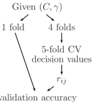
Next, for each instance in the validation set, we apply the pairwise coupling methods to obtain classification decisions. The error of the five validation sets is thus the cross-validation error at (C, γ). From this, each rule obtains its best (C, γ).2 Then, the decision values from the five-fold cross-validation at the best (C, γ) are employed in (33) to find the finalAandB for future use. These two values and the model via applying the best param-eters on the whole training set are then used to predict testing data. Figure 4 summarizes the procedure of getting validation accuracy at each given (C, γ).

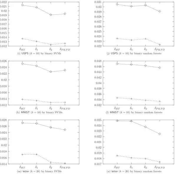
The average of 20 MSEs are presented on the left panel of Figure 5, where the solid line represents results of small sets (300 training/500 testing), and the dashed line of large sets (800 training/1,000 testing). The definition of MSE here is similar to (32), but as there is no correctpifor these problems, we letpi= 1 if the data is in theith class, and 0 otherwise. This measurement is called Brier Score (Brier, 1950), which is popular in meteorology. The figures show that for smallerk,δHT,δ1,δ2 andδP KP D have similar MSEs, but for larger k,

δHT has the largest MSE. The MSEs ofδV are much larger than those by all other methods, 2. If more than one parameter sets return the smallest cross-validation error, we simply choose the one

(14)

Given (C, γ) 1 fold 4 folds

5-fold CV decision values

rij validation accuracy

Figure 4: Parameter selection when using SVM as the binary classifier

so they are not included in the figures. In summary, the two proposed approaches,δ1andδ2, are fairly insensitive to the values ofk, and all above observations agree well with previous findings in Sections 5 and 6.

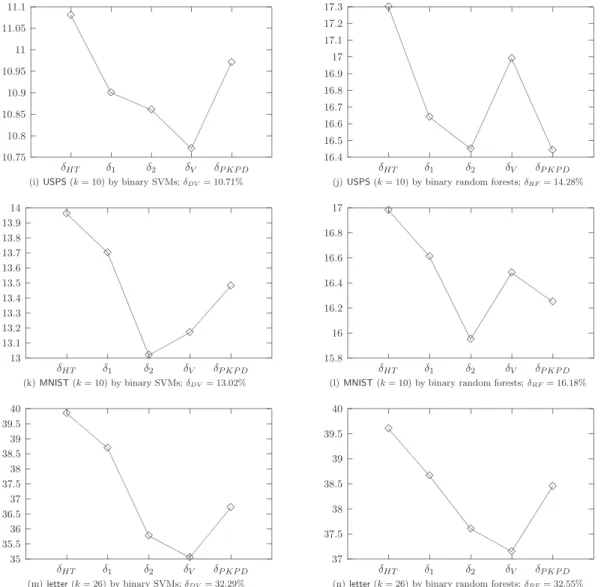
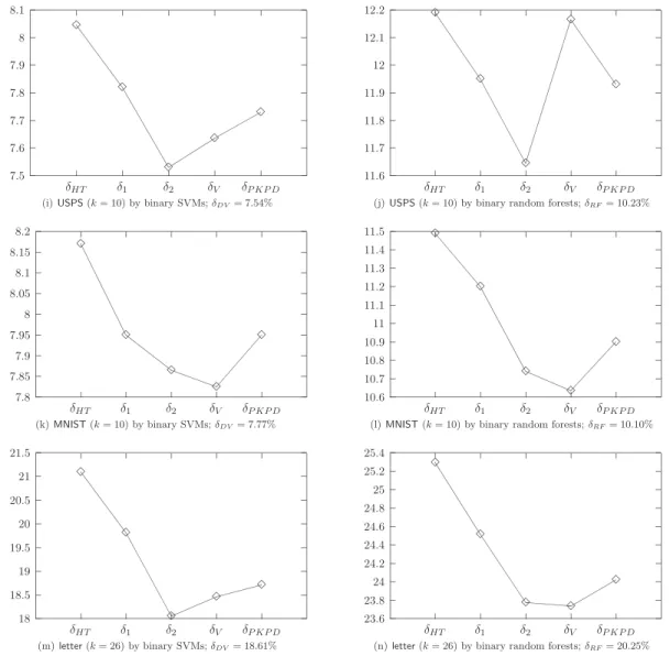
Next, left panels of Figures 6 and 7 present the average of 20 test errors for problems with small size (300 training/500 testing) and large size (800 training/1,000 testing), respectively. The caption of each sub-figure also shows the average of 20 test errors of the multi-class implementation inLIBSVM. This rule is voting using merely pairwise SVM decision values, and is denoted as δDV for later discussion. The figures show that the errors of the five methods are fairly close for smallerk, but quite different for largerk. Notice that for smaller

k(Figures 6 and 7 (a), (c), (e), and (g)) the differences of the averaged errors among the five methods are small, and there is no particular trend in these figures. However, for problems with larger k(Figures 6 and 7 (i), (k), and (m)), the differences are bigger and δHT is less competitive. In particular, for letterproblem (Figure 6 (m), k=26), δ2 and δV outperform

δHT by more than 4%. The test errors along with MSE seems to indicate that, for problems with larger k, the posterior probabilities pi are closer to the setting of Figure 2(c), rather than that of Figure 2(a). Another feature consistent with earlier findings is that when kis larger the results of δ2 are closer to those of δV, and δ1 closer to δHT, for both small and large training/testing sets. As for δP KP D, its overall performance is competitive, but we are not clear about its relationships to the other methods.

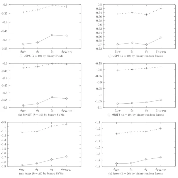
Finally, we consider another criterion on evaluating the probability estimates: the like-lihood.

l

Y

j=1

pj_y_j

In practice, we use its log likelihood and divide the value by a scaling factor l: 1

l

X

j=1

logpj_y_j, (34)

wherel is the number of test data, pj is the probability estimates for the jth data, andyj is its actual class label.

A larger value implies a possibly better estimate. The left panel of Figure 8 presents the results of using SVM as the binary classifier. Clearly the trend is the same as MSE and

(15)

accuracy. When k is larger, δ2 and δV have larger values and hence better performance. Similar to MSE, values of δV are not presented as they are too small.

7.2 Random Forest as the Binary Classifier

In this subsection we consider random forest (Breiman, 2001) as the binary classifier and conduct experiments on the same data sets. As random forest itself can provide multi-class probability estimates, we denote the corresponding rule as δRF and also compare it with the coupling methods.

For each two classes of data, we construct 500 trees as the random forest classifiers. Usingm_{try randomly selected features, a bootstrap sample (around two thirds) of training}

data are employed to generate a full tree without pruning. For each test instance, rij is simply the proportion out of the 500 trees that classiwins over classj. As we set the number of trees to be fixed at 500, the only parameter left for tuning is m_{try. Similar to (Sventnik}

et al., 2003), we selectm_{try from}_{1,√m, m/3, m/2, m_} by five-fold cross validation, where

m is the number of attributes. The cross validation procedure first sequentially uses four folds as the training set to constructk(k₋1)/2 pairwise random forests, next obtains the decision for each instance in the validation set by the pairwise coupling methods, and then calculates the cross validation error at the given m_{try by the error of five validation sets.}

This is similar to the procedure in Section 7.1, but we do not need a second-level CV for obtaining accurate two-class probabilistic estimates (i.e., rij). Instead of CV, a more efficient “out of bag” validation can be used for random forest, but here we keep using CV for consistency. Experiments are conducted using an R-interface (Liaw and Wiener, 2002) to the code from (Breiman, 2001).

The MSE presented in the right panel of Figure 5 shows thatδ1 andδ2yield more stable results thanδHT and δV for both small and large sets. The right panels of Figures 6 and 7 give the average of 20 test errors. The caption of each sub-figure also shows the averaged error when using random forest as a multi-class classifier (δRF). Notice that random forest bears a resemblance to SVM: the errors are only slightly different among the five methods for smaller k, butδV andδ2 tend to outperformδHT and δ1 for larger k. The right panel of Figure 8 presents the log likelihood value (34). The trend is again the same. In summary, the results by using random forest as the binary classifier strongly support previous findings regarding the four methods.

7.3 Miscellaneous Observations and Discussion

Recall that in Section 7.1 we considerδDV, which does not use Platt’s posterior probabilities. Experimental results in Figure 6 show that δDV is quite competitive (in particular, 3% better for letter), but is about 2% worse than all probability-based methods for waveform. Similar observations on waveform are also reported in (Duan and Keerthi, 2003), where the comparison is between δDV and δHT. We explain why the results by probability-based and decision-value-based methods can be so distinct. For some problems, the parameters selected byδDV are quite different from those by the other five rules. Inwaveform, at some parameters all probability-based methods gives much higher cross validation accuracy than

δDV. We observe, for example, the decision values of validation sets are in [0.73, 0.97] and [0.93, 1.02] for data in two classes; hence, all data in the validation sets are classified as

(16)

in one class and the error is high. On the contrary, the probability-based methods fit the decision values by a sigmoid function, which can better separate the two classes by cutting at a decision value around 0.95. This observation shed some light on the difference between probability-based and decision-value based methods.

Though the main purpose of this section is to compare different probability estimates, here we check the accuracy of another multi-class classification method: exponential loss-based decoding by Allwein et al. (2001). In the pairwise setting, if ˆfij ∈R is the two-class hypothesis so that ˆfij >0 (<0) predicts the data to be in theith (jth) class, then

predicted label = arg min i



 X

j:j<i

efˆji ₊ X

j:j>i

e−fˆij



. (35)

For SVM, we can simply use decision values as ˆfij. On the other hand,rij−1/2 is another choice. Table 2 presents the error of the seven problem using these two options. Results indicate that using decision values is worse than rij −1/2 when k is large (USPS,MNIST, andletter). This observation seems to indicate that large numerical ranges of ˆfij may cause (35) to have more erroneous results (rij−1/2 is always in [−1/2,1/2]). The results of using

rij−1/2 is competitive with those in Figures 6 and 7 whenkis small. However, for largerk (e.g.,letter), it is slightly worse thanδ2 andδV. We think this result is due to the similarity between (35) and δHT. When ˆfij is close to zero, efˆij ≈1 + ˆfij, so (35) reduces to a “linear loss-based encoding.” When rij−1/2 is used, ˆfji=rji−1/2 = 1/2−rij. Thus, the linear encoding is arg mini[P_j:j₆_=i−rij]≡arg maxi[P_j:j₆_=irij], exactly the same as (10) of δHT.

training/testing ( ˆfij) dna waveform satimage segment USPS MNIST letter 300/500 (dec. values) 10.47 16.23 14.12 6.21 11.57 14.99 38.59 300/500 (rij −1/2) 10.47 15.11 14.45 6.03 11.08 13.58 38.27 800/1000 (dec. values) 6.36 14.20 11.55 3.35 8.47 8.97 22.54 800/1000 (rij −1/2) 6.22 13.45 11.6 3.19 7.71 7.95 20.29 Table 2: Average of 20 test errors using exponential loss-based decoding (in percentage)

Regarding the accuracy of pairwise (i.e.,δDV) and non-pairwise (e.g., “one-against-the-rest”) multi-class classification methods, there are already excellent comparisons. As δV and δ2 have similar accuracy to δDV, roughly how non-pairwise methods compared toδDV is the same as compared toδV and δ2.

The results of random forest as a multi-class classifier (i.e., δRF) are reported in the caption of each sub-figure in Figures 6 and 7. We observe from the figures that, when the number of classes is larger, using random forest as a multi-class classifier is better than coupling binary random forests. However, for dna (k = 3) the result is the other way around. This observation for random forest is left as a future research issue.

(17)

The authors thank S. Sathiya Keerthi for helpful comments. They also thank the associate editor and anonymous referees for useful comments. This work was supported in part by the National Science Council of Taiwan via the grants NSC 90-2213-E-002-111 and NSC 91-2118-M-004-003.

References

Erin L. Allwein, Robert E. Schapire, and Yoram Singer. Reducing multiclass to binary: a unifying approach for margin classifiers. Journal of Machine Learning Research, 1: 113–141, 2001. ISSN 1533-7928.

C. L. Blake and C. J. Merz. UCI repository of machine learning databases. Technical report, University of California, Department of Information and Computer Science, Irvine, CA, 1998. Available at http://www.ics.uci.edu/~mlearn/MLRepository.html.

B. Boser, I. Guyon, and V. Vapnik. A training algorithm for optimal margin classifiers.

In Proceedings of the Fifth Annual Workshop on Computational Learning Theory, pages

144–152. ACM Press, 1992.

Leo Breiman. Random forests. Machine Learning, 45(1):5–32, 2001. URL citeseer.nj.

nec.com/breiman01random.html.

G. W. Brier. Verification of forecasts expressed in probabilities. Monthly Weather Review, 78:1–3, 1950.

Chih-Chung Chang and Chih-Jen Lin. LIBSVM: a library for support vector machines, 2001. Software available at http://www.csie.ntu.edu.tw/∼_cjlin/libsvm_.

Corina Cortes and Vladimir Vapnik. Support-vector network. Machine Learning, 20:273– 297, 1995.

Kaibo Duan and S. Sathiya Keerthi. Which is the best multiclass SVM method? An empirical study. Technical Report CD-03-12, Control Division, Department of Mechanical Engineering, National University of Singapore, 2003.

J. Friedman. Another approach to polychotomous classification. Technical report, Department of Statistics, Stanford University, 1996. Available at

http://www-stat.stanford.edu/reports/friedman/poly.ps.Z.

T. Hastie and R. Tibshirani. Classification by pairwise coupling. The Annals of Statistics, 26(1):451–471, 1998.

J. J. Hull. A database for handwritten text recognition research. IEEE Transactions on

Pattern Analysis and Machine Intelligence, 16(5):550–554, May 1994.

David R. Hunter. MM algorithms for generalized Bradley-Terry models. The Annals of

(18)

S. Knerr, L. Personnaz, and G. Dreyfus. Single-layer learning revisited: a stepwise procedure for building and training a neural network. In J. Fogelman, editor, Neurocomputing:

Algorithms, Architectures and Applications. Springer-Verlag, 1990.

Yann LeCun, L. Bottou, Y. Bengio, and P. Haffner. Gradient-based learning applied to doc-ument recognition. Proceedings of the IEEE, 86(11):2278–2324, November 1998. MNIST database available at http://yann.lecun.com/exdb/mnist/.

Andy Liaw and Matthew Wiener. Classification and regression by randomForest. R News, 2/3:18–22, December 2002. URL http://cran.r-project.org/doc/Rnews/

Rnews 2002-3.pdf.

Hsuan-Tien Lin, Chih-Jen Lin, and Ruby C. Weng. A note on Platt’s probabilistic outputs for support vector machines. Technical report, Department of Computer Science, Na-tional Taiwan University, 2003. URL http://www.csie.ntu.edu.tw/∼_{cjlin/papers/}

plattprob.ps.

D. Michie, D. J. Spiegelhalter, and C. C. Taylor. Machine Learning, Neural and Statistical

Classification. Prentice Hall, Englewood Cliffs, N.J., 1994. Data available at http:

//www.ncc.up.pt/liacc/ML/statlog/datasets.html.

J. Platt. Probabilistic outputs for support vector machines and comparison to regularized likelihood methods. In A.J. Smola, P.L. Bartlett, B. Sch¨olkopf, and D. Schuurmans, editors, Advances in Large Margin Classifiers, Cambridge, MA, 2000. MIT Press. URL

citeseer.nj.nec.com/platt99probabilistic.html.

David Price, Stefan Knerr, L´eon Personnaz, and G´erard Dreyfus. Pairwise nerual network classifiers with probabilistic outputs. In G. Tesauro, D. Touretzky, and T. Leen, editors,

Neural Information Processing Systems, volume 7, pages 1109–1116. The MIT Press,

1995.

Ph. Refregier and F. Vallet. Probabilistic approach for multiclass classification with neural networks. InProceedings of International Conference on Artificial Networks, pages 1003– 1007, 1991.

Sheldon Ross. Stochastic Processes. John Wiley & Sons, Inc., second edition, 1996.

Vladimir Sventnik, Andy Liaw, Christopher Tong, J. Christopher Culberson, Robert P. Sheridan, and Bradley P. Feuston. Random forest: a tool for classification and regression in compound classification and QSAR modeling. Journal of Chemical Information and

Computer Science, 43(6):1947–1958, 2003.

Ting-Fan Wu, Chih-Jen Lin, and Ruby C. Weng. Probability estimates for multi-class classification by pairwise coupling. In Sebastian Thrun, Lawrence Saul, and Bernhard Sch¨olkopf, editors, Advances in Neural Information Processing Systems 16. MIT Press, Cambridge, MA, 2004.

E. Zermelo. Die Berechnung der Turnier-Ergebnisse als ein Maximumproblem der Wahrscheinlichkeitsrechnung. Mathematische Zeitschrift, 29:436–460, 1929.

(19)

Tong Zhang. Statistical behavior and consistency of classification methods based on convex risk minimization. The Annals of Statistics, 32(1):56–134, 2004.

Appendix A. Proof of Theorem 2

It suffices to prove that any optimal solution p of (18) satisfiespi ≥0, i= 1, . . . , k. If this is not true, without loss of generality, we assume

p1 ≤0, . . . , pr≤0, pr+1 >0, . . . , pk>0,

where 1 _≤r < k, and there is one 1 _≤i_≤ r such that pi <0. We can then define a new feasible solution of (18):

p′₁ = 0, . . . , p′_r= 0, p_r+1′ =pr+1/α, . . . , p′k=pk/α, whereα= 1₋Pr

i=1pi >1.

With rij >0 andrji>0, we obtain

(rjipi−rijpj)2 ≥0 = (rjip′i−rijp′j)2, if 1≤i, j≤r, (rjipi−rijpj)2 = (rijpj)2>

(rijpj)2

α2 = (rjip ′

i−rijp′j)2, if 1≤i≤r, r+ 1≤j≤k, (rjipi−rijpj)2 ≥

(rjipi−rijpj)2

α2 = (rjip ′

i−rijp′j)2, ifr+ 1≤i, j≤k. Therefore,

k

X

i=1

X

j:j6=i

(rijpi−rjipj)2> k

X

i=1

X

j:j6=i

(rijp′i−rjip′j)2. This contradicts the assumption that p is an optimal solution of (18).

Appendix B. Proof of Theorem 3

(i) IfQ+ ∆eeT _{is not positive definite, there is a vector} _v _with_v

i 6= 0 such that

vT(Q+ ∆eeT)v= 1 2

k

X

t=1

X

u:u6=t

(rutvt−rtuvu)2+ ∆( k

X

t=1

vt)2 = 0. (36) For allt₆=i,ritvt−rtivi = 0, so

vt=

rti

rit

vi 6= 0. Thus,

k

X

t=1

vt= (1 +

X

t:t6=i

rti

rit

)vi6= 0, which contradicts (36).

(20)

The positive definiteness of Q + ∆eeT _{implies that} hQ+∆eeT e eT 0 i

is invertible. As h

Q+∆eeT e eT 0 i

is from adding the last row of hQ e eT 0 i

to its first k rows (with a scaling factor ∆), the two matrices have the same rank. Thus, hQ e

eT 0 i

is invertible as well. Then (21) has a unique solution, and so does (17).

(ii) IfQis not positive definite, there is a vector v withvi 6= 0 such that

vTQv= 1 2

k

X

t=1

X

u:u6=t

(rutvt−rtuvu)2= 0. Therefore,

(rutvt−rtuvu)2 = 0,∀t6=u.

Asrtu>0,∀t6=u, for anys6=j for which s6=iand j6=i, we have

vs=

rsi

ris

vi, vj =

rji

rij

vi, vs=

rsj

rjs

vj. (37)

Asvi6= 0, (37) implies

rsirjs

ris

= rjirsj

rij

,

which contradicts (22).

Appendix C. Proof of Theorem 4

First we need a lemma to show the strict decrease of the objective function:

Lemma 5 If rij >0,∀i6=j, p and pn are from two consecutive iterations of Algorithm 2,

and pn₆₌_p_{, then}

1 2(p

n₎T_Q_pn_< 1 2p

T_Q_p_. ₍₃₈₎

Proof.Assume that ptis the component to be updated. Then, pn is obtained through the following calculation:

¯

pi=

(

pi ifi6=t,

1 Qtt(−

P

j:j6=tQtjpj+pTQp) ifi=t,

(39) and

pn= p¯ Pk

i=1p¯i

. (40)

For (40) to be a valid operation, Pk

i=1p¯i must be strictly positive. To show this, we first suppose that the current solution p satisfies pi ≥ 0, i = 1, . . . , l, but the next solution ¯p has Pk

i=1p¯i = 0. In Section 4.2, we have shown that ¯pt ≥ 0, so with ¯pi =pi ≥ 0,∀i 6= t, ¯

pi = 0 for all i. Next, from (39), pi = ¯pi = 0 for i 6=t, which, together with the equality

Pk

(21)

(39). This contradicts the situation that ¯pi = 0 for alli. Therefore, by induction, the only requirement is to have nonnegative initialp.

To prove (38), first we rewrite the update rule (39) as ¯

pt = pt+ 1

Qtt

(₋(Qp)t+pTQp) (41)

= pt+ ∆. Since we keep Pk

i=1pi= 1, Pk_i=1p¯i = 1 + ∆. Then

¯

pTQp¯₋( k

X

i=1 ¯

pi)2pTQp

= pTQp+ 2∆(Qp)t+Qtt∆2−(1 + ∆)2pTQp = 2∆(Qp)t+Qtt∆2−(2∆ + ∆2)pTQp = ∆ 2(Qp)t−2pTQp+Qtt∆−∆pTQp

= ∆(₋Qtt∆−∆pTQp) (42)

= ₋∆2(Qtt+pTQp)<0. (43)

(42) follows from the definition of ∆ in (41). For (43), it uses Qtt = P_j:j₆_=tr2jt > 0 and ∆₆= 0, which comes from the assumptionpn₆₌_p_. ₂

Now we are ready to prove the theorem. If this result does not hold, there is a convergent sub-sequence_{pi_}

i∈K such thatp∗ = limi∈K,i→∞pi is not optimal for (17). Note that there

is at least one index of_{1, . . . , k_}which is considered in infinitely many iterations. Without loss of generality, we assume that for all pi_{, i} _∈ _K_, _pi

t is updated to generate the next iterationpi+1_{. As}_p∗ _{is not optimal for (17), starting from}_{t, t}_{+ 1}_{, . . . , k,}₁_{, . . . , t}₋_{1, there}

is a first component ¯t for which k

X

j=1

Q¯tjp∗j −(p∗)TQp∗ 6= 0. By applying one iteration of Algorithm 2 onp∗

¯

t, from an explanation similar to the proof of Lemma 5, we obtain p∗,n satisfying p_t_¯∗,n ₆=p∗t¯. Then by Lemma 5,

1 2(p

∗,n₎T_Q_p∗,n _< 1 2(p

∗₎T_Q_p∗_.

Assume it takes ¯isteps from tto ¯t and ¯i >1, lim

i∈K,i→∞p i+1

t = lim

i∈K,i→∞

1 Qtt(−

P

j:j6=tQtjpit+ (pi)TQpi) 1

Qtt(−

P

j:j6=tQtjpit+ (pi)TQpi) +

P

j:j6=tpij =

1 Qtt(−

P

j:j6=tQtjp∗t + (p∗)TQp∗) 1

Qtt(−

P

j:j6=tQtjp∗t + (p∗)TQp∗) +

P

j:j6=tp∗j

= p

∗ t

Pk

j=1p∗j =p∗_t,

(22)

we have

lim i∈K,i→∞p

i₌ _lim i∈K,i→∞p

i+1 ₌

· · ·= lim i∈K,i→∞p

i+¯i−1 ₌_p∗_.

Moreover,

lim i∈K,i→∞p

i+¯i ₌_p∗,n and

lim i∈K,i→∞

1 2(p

i+¯i₎T_Q_pi+¯i ₌ 1 2(p

∗,n₎T_Q_p∗,n

< 1

2(p

∗₎T_Q_p∗

= lim

i∈K,i→∞

1 2(p

i₎T_Q_pi_. This contradicts the fact from Lemma 5:

1 2(p

1₎T_Q_p1

≥ 1₂(p2)TQp2 _{≥ · · · ≥} 1 2(p

∗₎T_Q_p∗_.

Therefore, p∗ _{must be optimal for (17).}

Appendix D. Implementation Notes of Algorithm 2

From Algorithm 2, the main operation of each iteration is on calculating ₋P

j:j6=tQtjpj andpT_Q_p_{, both}_O₍_k2_{) procedures. In the following, we show how to easily reduce the cost} per iteration toO(k).

Following the notation in Lemma 5 of Appendix D, we considerp the current solution. Assumeptis the component to be updated, we generate ¯paccording to (39) and normalize ¯

p to the next iterate pn_{. Note that ¯}_p _{is the same as} _p _{except the}_t_{th component and we} consider the form (41). SincePk

i=1pi= 1, (40) is pn= ¯p/(1 + ∆). Throughout iterations, we keep the current Qp and pT_Q_p_{, so ∆ can be easily calculated. To obtain} _Q_pn _and (pn₎T_Q_pn_{, we use}

(Qpn)j =

(Qp¯)j 1 + ∆

= (Qp)j +Qjt∆

1 + ∆ , j = 1, . . . , k, (44)

and

(pn)TQ(pn) = p¯ T_Q_p_¯

(1 + ∆)2 (45)

= p

T_Q_p_{+ 2∆}Pk

j=1(Qp)j +Qtt∆2

(1 + ∆)2 .

Both (and hence the whole iteration) takes O(k) operations.

Numerical inaccuracy may accumulate through iterations, so gradually (44) and (45) may be away from values directly calculated using p. An easy prevention of this problem is to recalculate Qp and pTQp directly using p after several iterations (e.g., k iterations). Then, the average cost per iteration is stillO(k) +O(k2)/k=O(k).

(23)

Appendix E. Derivation of (29) k

X

i=1

X

j:j6=i

(I_{rij>rji}pj−I{rji>rij}pi)

2

= k

X

i=1

X

j:j6=i

(I_{_r_ij_>r_ji_}p2_j+I_{_r_ji_>r_ij_}p2_i)

= 2 k

X

i=1 (X

j:j6=i

I{rji>rij})p

2 i.

If P

j:j6=iI{rji>rij} 6= 0,∀i, then, under the constraint

Pk

i=1pi = 1, the optimal solution satisfies

p1

P

j:j6=1I{rj1>r1j}

=_{· · ·}= P pk

j:j6=kI{rjk>rkj} .

(24)

0.03 0.035 0.04 0.045 0.05 0.055

δHT δ1 δ2 δP KP D

3

3 ₃ 3

+ + + +

(a)dna(k= 3) by binary SVMs

0.04 0.041 0.042 0.043 0.044 0.045 0.046 0.047 0.048 0.049

3

3 3 3

+ +

+

(b)dna(k= 3) by binary random forests

0.065 0.066 0.067 0.068 0.069 0.07 0.071 0.072 0.073

3 3 3 ₃

+ + + +

(c)waveform(k= 3) by binary SVMs

0.082 0.084 0.086 0.088 0.09 0.092 0.094

3 3 3 3 + + + +

(d)waveform(k= 3) by binary random forests

0.027 0.028 0.029 0.03 0.031 0.032 0.033 0.034 0.035 0.036 0.037

3 3 3 ₃

+ + + +

(e)satimage(k= 6) by binary SVMs

0.032 0.033 0.034 0.035 0.036 0.037 0.038 0.039 0.04

3 3 3 3 + + + +

(f)satimage(k= 6) by binary random forests

0.008 0.01 0.012 0.014 0.016 0.018 0.02

3 3

3 ₃

+ ₊

(g)segment(k= 7) by binary SVMs

0.008 0.009 0.01 0.011 0.012 0.013 0.014 0.015

3 3

+ + +

+

(25)

0.012 0.013 0.014 0.015 0.016 0.017 0.018 0.019 0.02 0.021 0.022

3 3

+ +

(i)USPS(k= 10) by binary SVMs

0.022 0.023 0.024 0.025 0.026 0.027 0.028 0.029 0.03 0.031

3 ₃ 3

3

+ ₊ +

+

(j)USPS(k= 10) by binary random forests

0.012 0.014 0.016 0.018 0.02 0.022 0.024 0.026

3 3

+ ₊

+ +

(k)MNIST(k= 10) by binary SVMs

0.032 0.034 0.036 0.038 0.04 0.042 0.044 0.046 0.048

3 ₃

+ ₊

(l)MNIST(k= 10) by binary random forests

0.014 0.016 0.018 0.02 0.022 0.024 0.026 0.028

3 3

+ +

+ ₊

(m)letter(k= 26) by binary SVMs

0.017 0.018 0.019 0.02 0.021 0.022 0.023 0.024 0.025

3 3

+

+ ₊

+

(n)letter(k= 26) by binary random forests

Figure 5: MSE by using four probability estimates methods based on binary SVMs (left) and binary random forests (right). MSE of δV is too large and is not presented. solid line: 300 training/500 testing points; dotted line: 800 training/1,000 testing points.

(26)

10.35 10.4 10.45 10.5 10.55 10.6 10.65

δHT δ1 δ2 δV δP KP D

3 3

3

(a)dna(k= 3) by binary SVMs;δDV= 10.82%

7.4 7.5 7.6 7.7 7.8 7.9 8 8.1 8.2

3 3

3

(b)dna(k= 3) by binary random forests;δRF= 8.74%

14.8 14.81 14.82 14.83 14.84 14.85 14.86 14.87 14.88 14.89

3

3 3

3

(c)waveform(k= 3) by binary SVMs;δDV= 16.47%

17.1 17.2 17.3 17.4 17.5 17.6 17.7 17.8 17.9

3 3

3

(d)waveform(k= 3) by binary random forests;δRF= 17.39%

14.2 14.3 14.4 14.5 14.6 14.7 14.8 14.9

3

3 3

3

(e)satimage(k= 6) by binary SVMs;δDV= 14.88%

14.7 14.8 14.9 15 15.1 15.2 15.3 15.4 15.5 15.6

3

3 3

(f)satimage(k= 6) by binary random forests;δRF= 14.74%

5.75 5.8 5.85 5.9 5.95 6 6.05 6.1 6.15 6.2 6.25 6.3

3

3 3

3

(g)segment(k= 7) by binary SVMs;δDV= 5.82%

5.3 5.4 5.5 5.6 5.7 5.8 5.9 6

3

3 3

3

(27)

10.75 10.8 10.85 10.9 10.95 11 11.05 11.1

3

3 3

(i)USPS(k= 10) by binary SVMs;δDV= 10.71%

16.4 16.5 16.6 16.7 16.8 16.9 17 17.1 17.2 17.3

3

3 3

3

(j)USPS(k= 10) by binary random forests;δRF= 14.28%

13 13.1 13.2 13.3 13.4 13.5 13.6 13.7 13.8 13.9 14

3 3

3

(k)MNIST(k= 10) by binary SVMs;δDV= 13.02%

15.8 16 16.2 16.4 16.6 16.8 17

3

3 3

3

(l)MNIST(k= 10) by binary random forests;δRF= 16.18%

35 35.5 36 36.5 37 37.5 38 38.5 39 39.5 40

3 3

3

(m)letter(k= 26) by binary SVMs;δDV= 32.29%

37 37.5 38 38.5 39 39.5 40

3

3 3

3

(n)letter(k= 26) by binary random forests;δRF= 32.55%

Figure 6: Average of 20 test errors by five probability estimates methods based on binary SVMs (left) and binary random forests (right). Each of the 20 test errors is by 300 training/500 testing points. Caption of each sub-figure shows the averaged error by voting using pairwise SVM decision values (δDV) and the multi-class random forest (δRF).

(28)

6.2 6.25 6.3 6.35 6.4 6.45 6.5 6.55

3 3

3

(a)dna(k= 3) by binary SVMs;δDV= 6.31%

5.84 5.86 5.88 5.9 5.92 5.94 5.96 5.98 6 6.02 6.04

3 3

3

3 3

(b)dna(k= 3) by binary random forests;δRF= 6.91%

13.54 13.55 13.56 13.57 13.58 13.59 13.6 13.61

3 3

3

(c)waveform(k= 3) by binary SVMs;δDV= 14.33%

15.7 15.75 15.8 15.85 15.9 15.95 16

3 3 ₃

3

(d)waveform(k= 3) by binary random forests;δRF= 15.66%

11.44 11.46 11.48 11.5 11.52 11.54 11.56 11.58

3 3

3

(e)satimage(k= 6) by binary SVMs;δDV= 11.54%

12.1 12.2 12.3 12.4 12.5 12.6 12.7

3 3

3

(f)satimage(k= 6) by binary random forests;δRF= 11.92%

3.05 3.1 3.15 3.2 3.25 3.3 3.35

3

3 3

3

(g)segment(k= 7) by binary SVMs;δDV= 3.30%

3.45 3.5 3.55 3.6 3.65 3.7 3.75 3.8

3

3 3

3

(29)

7.5 7.6 7.7 7.8 7.9 8 8.1

3

3 3

3

(i)USPS(k= 10) by binary SVMs;δDV= 7.54%

11.6 11.7 11.8 11.9 12 12.1 12.2

3

3 3

3

(j)USPS(k= 10) by binary random forests;δRF= 10.23%

7.8 7.85 7.9 7.95 8 8.05 8.1 8.15 8.2

3

3 3

(k)MNIST(k= 10) by binary SVMs;δDV= 7.77%

10.6 10.7 10.8 10.9 11 11.1 11.2 11.3 11.4 11.5

3

3 3

3

(l)MNIST(k= 10) by binary random forests;δRF= 10.10%

18 18.5 19 19.5 20 20.5 21 21.5

3

3 3

(m)letter(k= 26) by binary SVMs;δDV= 18.61%

23.6 23.8 24 24.2 24.4 24.6 24.8 25 25.2 25.4

3

3 ₃

3

(n)letter(k= 26) by binary random forests;δRF= 20.25%

Figure 7: Average of 20 test errors by five probability estimates methods based on binary SVMs (left) and binary random forests (right). Each of the 20 test errors is by 800 training/1,000 testing points. Caption of each sub-figure shows the averaged error by voting using pairwise SVM decision values (δDV) and the multi-class random forest (δRF).

(30)

-0.28 -0.26 -0.24 -0.22 -0.2 -0.18 -0.16

3 3 3 3

+ + ₊ ₊

(a)dna(k= 3) by binary SVMs

-0.31 -0.3 -0.29 -0.28 -0.27 -0.26 -0.25

3

3 3 3

+

+ +

(b)dna(k= 3) by binary random forests

-0.365 -0.36 -0.355 -0.35 -0.345 -0.34 -0.335 -0.33 -0.325 -0.32

3

3 3 3

+

+ + +

(c)waveform(k= 3) by binary SVMs

-0.48 -0.47 -0.46 -0.45 -0.44 -0.43 -0.42 -0.41

3 3 3 3 + + + +

(d)waveform(k= 3) by binary random forests

-0.44 -0.42 -0.4 -0.38 -0.36 -0.34 -0.32

3 ₃ ₃ 3

+ + + +

(e)satimage(k= 6) by binary SVMs

-0.5 -0.48 -0.46 -0.44 -0.42 -0.4 -0.38

3 3

+

+ +

+

(f)satimage(k= 6) by binary random forests

-0.32 -0.3 -0.28 -0.26 -0.24 -0.22 -0.2 -0.18 -0.16 -0.14 -0.12

3 3

+ +

(g)segment(k= 7) by binary SVMs

-0.22 -0.21 -0.2 -0.19 -0.18 -0.17 -0.16 -0.15 -0.14 -0.13

3 3 3 3

+ + ₊ +

(31)

-0.55 -0.5 -0.45 -0.4 -0.35 -0.3

3 3

3 ₃

+ +

+ ₊

(i)USPS(k= 10) by binary SVMs

-0.72 -0.7 -0.68 -0.66 -0.64 -0.62 -0.6 -0.58 -0.56 -0.54 -0.52 -0.5

3 3 3

3

+ + +

+

(j)USPS(k= 10) by binary random forests

-0.6 -0.55 -0.5 -0.45 -0.4 -0.35 -0.3

3 3

3 ₃

+ +

(k)MNIST(k= 10) by binary SVMs

-1.1 -1.05 -1 -0.95 -0.9 -0.85 -0.8 -0.75

3 3 3 3

+ + + +

(l)MNIST(k= 10) by binary random forests

-1.9 -1.8 -1.7 -1.6 -1.5 -1.4 -1.3 -1.2 -1.1 -1 -0.9

3 3

+ +

(m)letter(k= 26) by binary SVMs

-1.8 -1.7 -1.6 -1.5 -1.4 -1.3 -1.2 -1.1

3 3

+ + +

+

(n)letter(k= 26) by binary random forests

Figure 8: Log likelihood (34) by using four probability estimates methods based on binary SVMs (left) and binary random forests (right). MSE of δV is too small and is not presented. solid line: 300 training/500 testing points; dotted line: 800 training/1,000 testing points.