Volume 61 (2013)
Selected Revised Papers from the
4th International Workshop on
Graph Computation Models
(GCM 2012)
Verifying Total Correctness of Graph Programs
Christopher M. Poskitt and Detlef Plump 20 pages
Guest Editors: Rachid Echahed, Annegret Habel, Mohamed Mosbah Managing Editors: Tiziana Margaria, Julia Padberg, Gabriele Taentzer
Verifying Total Correctness of Graph Programs
Christopher M. Poskitt1and Detlef Plump2
1ETH Z¨urich, Switzerland 2The University of York, UK
Abstract: GP 2 is an experimental nondeterministic programming language based on graph transformation rules, allowing for visual programming and the solving of graph problems at a high-level of abstraction. In previous work we demonstrated how to verify graph programs using a Hoare-style proof calculus, but only partial correctness was considered. In this paper, we add new proof rules and termination functions, which allow for proofs to additionally guarantee that program executions always terminate (weak total correctness), or that programs always terminate and do so without failure (total correctness). We show that the new proof rules are sound with respect to the operational semantics of GP 2, complete for termination, and demonstrate their use on some example programs.
Keywords:graph programs, verification, Hoare logic, total correctness, termination
1
Introduction
The verification of graph transformation systems is an area of active and growing interest, mo-tivated by the many applications of graph transformation to specification and programming. Whilst much of the research in this area has focused on sets of rules or graph grammars (see e.g. [BCK08, BHE09, KE10, CR12]), the challenge of verifying graph-based programming languages is also beginning to be addressed. In particular, Habel, Pennemann, and Rensink [HPR06,HP09] contributed a verification framework – based on weakest preconditions – for a simple graph transformation language, expressing graph properties with nested conditions (a formalism based on graph morphisms). Their language however does not support important prac-tical features such as computation on labels, and their weakest precondition calculus generates infinite preconditions for loops.
numbers) in the new proof rule for the iteration command. We demonstrate the proof calculi on programs that have loops and potential failure points, before proving the calculi to be sound as well as complete for termination.
In contrast to our previous papers, we present the work here in the setting of GP 2 [Plu12] (henceforth referred to as simply GP). This extended version of the language has an improved type system, a marking (shading) mechanism for nodes and edges, a new conditional construct, and a simplified semantics for branching and iteration to support a more efficient implementation. Our previous verification work has been updated in [Pos13] to support these new features, but due to space limitations we cannot present all of the revised definitions here. We attempt to make the intuition behind each concept clear, but refer the interested reader to [Pos13] for the full technical details and further explanations.
Section2reviews some technical preliminaries. Section3is an informal introduction to graph programs. Section4reviews our assertion language and the partial correctness proof rules of our previous calculus. Section5formalises the notion of (weak) total correctness and presents new proof rules which allow one to prove these properties. Section6demonstrates the use of the new calculi on some example programs. Section7presents a proof that the new calculi are sound for (weak) total correctness, and also a proof that the calculi are complete for termination. Finally, we conclude in Section8.
This paper is a revised and extended version of [PP12b].
2
Preliminaries
Graph transformation in GP is based on the double-pushout (DPO) approach with relabelling [HP02], i.e. an approach in which both node and edge labels can be relabelled. This framework deals with rules containing partially labelled graphs, the definition of which we recall below. In this section we treat the label alphabet as a parameter because we will require two different alphabets for two classes of graphs: “syntactic” graphs labelled with expressions, and “semantic” graphs labelled with lists composed of integers and strings. We also introduce assignments which translate syntactic graphs into semantic graphs.
Agraphover a label alphabetC is a systemG= (VG,EG,sG,tG,lG,mG), whereVGandEGare finite sets ofnodes(orvertices) andedges,sG,tG:EG→VGare thesourceandtargetfunctions
for edges,lG:VG→C is the partial1node labelling function andmG:EG→C is the (total) edge
labelling function (edges can be relabelled by deletion and re-insertion, hence unlabelled edges are not necessary). Given a nodev, we writelG(v) =⊥to express thatlG(v)is undefined. Graph
Gistotally labelled iflG is a total function. We writeG(C) for the set of all totally labelled
graphs overC, andG(C⊥)for the set of all graphs overC. Theempty graph, denoted by /0, has empty node and edge sets.
A graph morphism g: G→ H between graphs G,H in G(C⊥) consists of two functions gV:VG→VH and gE:EG →EH that preserve sources, targets and labels; that is, sH◦gE =
gV ◦sG,tH◦gE =gV ◦tG, mH◦gE =mG, andlH(g(v)) =lG(v) for all v such thatlG(v)6=⊥.
Morphismgis aninclusionifg(x) =xfor all nodes and edgesx. It isinjective(surjective) ifgV
andgE are injective (surjective). It is anisomorphismif it is injective, surjective, and satisfies
lH(gV(v)) =⊥for all nodesv withlG(v) =⊥. In this caseGandH areisomorphic, which is
denoted byG∼=H.
We consider graphs over two distinct label alphabets. Graph programs and our assertion lan-guage contain graphs labelled with expressions, while the graphs on which programs operate are labelled with lists composed of integers and character strings. In both cases nodes and edges can be marked; marked nodes are displayed as shaded, and marked edges are displayed as dashed (see Figure2). We consider graphs of the first type as syntactic objects and graphs of the second type as semantic objects, and aim to clearly separate these levels of syntax and semantics.
LetZdenote the set of integers and Char a finite set of characters. We fix the label alphabet: L = (Z∪Char∗)∗×B
where B={true,false}, i.e. all sequences over integers and character strings, along with a
Boolean value indicating whether the node or edge is marked or not. Occasionally we will refer only to the list component(Z∪Char∗)∗, which shall be denoted byL.
The other label alphabet we are using, Label, consists of a mark component and (colon de-limited) sequences of arithmetical expressions and strings. These may contain variables from a set denoted by VarId. Variables represent values inL, i.e. lists, and can be constrained in rule
schemata to represent integers, strings, or atoms (an integer or a string). These types correspond to the semantic domains in Figure1, in which we identify atoms and unit-length lists to establish a subtype hierarchy.
list
atom
int string
⊆
⊆ ⊇
(Z∪Char∗)∗
Z∪Char∗
Z Char∗
⊆
⊆ ⊇
Figure 1: Subtype hierarchy for lists
We writeG(Label)to denote the set of all graphs labelled over Label (grammars defining the label alphabet are given in [Plu12,Pos13]). Examples of list components of labels inG(Label) includex*5and ”root” :y(the variable xmay only be instantiated to integers, whereasybe instantiated to any value inL, unless otherwise constrained).
Each graph inG(Label) represents a possibly infinite set of graphs inG(L). The latter are obtained by instantiating variables with values fromLand evaluating expressions. An
assign-mentis a partial functionα: VarId→L. For a rule schema (see the next section),α must satisfy for all variablesxwith typeint(resp.string,atom,list),α(x)∈Z(resp. Char∗,Z∪Char∗, L). For assertions (see Section4), we require thatα iswell-typedfor the expressions to which it
Given a (well-typed) assignmentαand label(e b)withea list andb∈B, we define(e b)α=
(eα,b) where the valueeα ∈Lis inductively defined as follows. Ifeis the empty list, theneα
is the empty sequence. Ifeis a numeral or a sequence of characters, theneα is the integer or character string represented bye. (Note that the empty list and empty character string are distinct values.) Ifeis a variable identifier, theneα=α(e). For arithmetic and string expressions,eα is defined inductively in the usual way. Finally, ifehas the forme1:e2withe1,e2list expressions, theneα =eα1eα2 (the concatenation of the sequenceseα1 andeα2). Given a graph GinG(Label) and an assignmentαwell-typed for all expressions inG, we writeGαfor the graph inG(L)that is obtained fromGby replacing each labellwithlα (note thatGα has the same nodes, edges, source and target functions asG). Ifg:G→His a graph morphism withG,H∈G(Label), then gαdenotes the morphismhgV,gEi:Gα→Hα.
Remark1 In [Plu12], variables belong to one of four distinct sets of variables – one set for each type – and assignments are families of mappings from the these sets to the appropriate semantic domains. We use a different definition in this paper, taking all variables to be members of the set VarId, and interpreting type declarations in rule schemata as constraints on possible assignments. This definition allows us to treat variables in rule schemata and our assertion language more uni-formly, simplifying the presentation of this paper. Additionally, though GP 2 introduced indegree and outdegree functions in expressions, we do not consider them in this paper, as applicability properties of rule schemata that use them cannot be expressed by our assertion language.
3
Graph Programs
We introduce graph programs informally and by example in this section. For technical details, further examples, and more discussion on the operational semantics, refer to [Plu12].
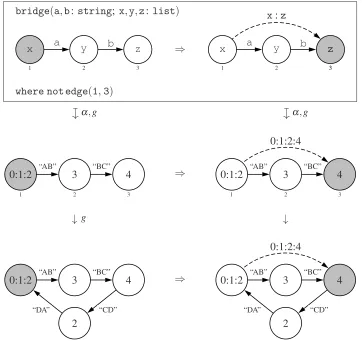
The “building blocks” of graph programs are (conditional) rule schemata: a program is es-sentially a list of declarations of (conditional) rule schemata together with a command sequence for controlling their application. Rule schemata generalise graph transformation rules, in that labels contain (sequences of) expressions and relabelling is supported. Expressions may con-tain variables, which in rule schemata are associated with types integer, string, atom, or list, constraining the possible mappings for assignments. Conditional rule schemata further con-strain assignments with a condition: one use is in requiring relations between expressions (e.g. x<y+z), but they can also be used to require (the absence of) edges between nodes in a match (e.g.not edge(1,2)). As the values of variables at execution are determined by graph match-ing, we require that expressions in the left graph have a simple shape: (1) expressions contain no arithmetic operators; (2) expressions contain at most one occurrence of a list variable; and (3) each string expression contains at most one occurrence of a string variable.
the first node to the third (as per the condition). The effect of applyingbridgeis to add a marked edge from the first node to the third, removing the mark from the former whilst adding a mark to the latter, and taking the composition of their list components for the new edge. The conditional rule schema describes an infinite number of “concrete” graph transformation rules with labels fitting the pattern described by the schema. The second row of the diagram shows one such rule, obtained by evaluating expressions according to the assignment:
α={a7→“AB”,b7→“BC”,x7→0 : 1 : 2,y7→3,z7→4}
which adheres to the constraints of the type declaration. The bottom row shows an application ofbridgeto a graph via the same assignmentα and an injective morphismg. It is applied in the double-pushout approach with relabelling [HP02], which intuitively means that nodes can be relabelled in an arbitrary context (edges can simply be deleted and reinserted with the new labels), and that the application is side-effect free (i.e. it is forbidden to delete a node unless the rule schema explicitly deletes all edges it is incident to).
bridge(a,b:string; x,y,z:list)
x
1
y
2
z
3
a b
⇒ x
1
y
2 3
z
3
x:z
a b
where not edge(1,3)
7→
α,g 7→ α,g
0:1:2
1
3
2
4
3
“AB” “BC”
⇒ 0:1:2
1
3
2
4
3
0:1:2:4 “AB” “BC”
↓ g ↓
0:1:2 3 4
2
“AB” “BC”
“CD” “DA”
⇒ 0:1:2 3 4
2 0:1:2:4 “AB” “BC”
“CD” “DA”
Figure 2: A conditional rule schema and a possible application of it
H∈G(L), denotedG⇒rH, proceeds roughly as follows:
1. Match the left graphLofrwith a subgraph ofG, ignoring labels, by means of a so-called premorphism g:L→ G. (A premorphism is a graph morphism that does not need to preserve labels.)
2. Check whether there is an assignmentα of values to all the variables inr(adhering to the declared types) such that after evaluating the expressions inL,gis label-preserving. 3. Ifris a conditional rule schema, check that the condition evaluates to true with respect to
αandg(conditions are evaluated in the obvious way, withedge(m,n)α,g=true for node identifiersm,nif and only if there is an edge with sourcegV(m)and targetgV(n)).
4. Apply the rule rα (obtained from r by evaluating2 all expressions in the left and right graph) toGwith matchgvia the double-pushout approach with relabelling.
We also writeG⇒R H for a set of (conditional) rule schemataRif there is somer∈R such
thatG⇒rH.
Declarations of (conditional) rule schemata are, in graph programs, applied according to a number of simple control constructs. GP provides non-deterministic choice, sequential compo-sition, conditional constructs, and as-long-as-possible iteration. We demonstrate these informally with two example programs.
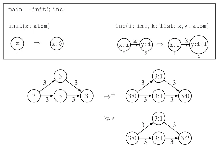
The programcolouring in Figure3produces a colouring (assignment of integers to nodes such that adjacent nodes have different colours), provided that the input graph consists of un-marked items only, and the list components of nodes are atomic. Colours are recorded as so-called tags, i.e. information stored in a label by extending the list component.
The program initially colours each node with 0 by applying the rule schemainitas long as possible, using the iteration operator ’!’. It then repeatedly increments the target colour of edges with the same colour at both ends. Note that this process is nondeterministic: Figure3shows two possible executions.
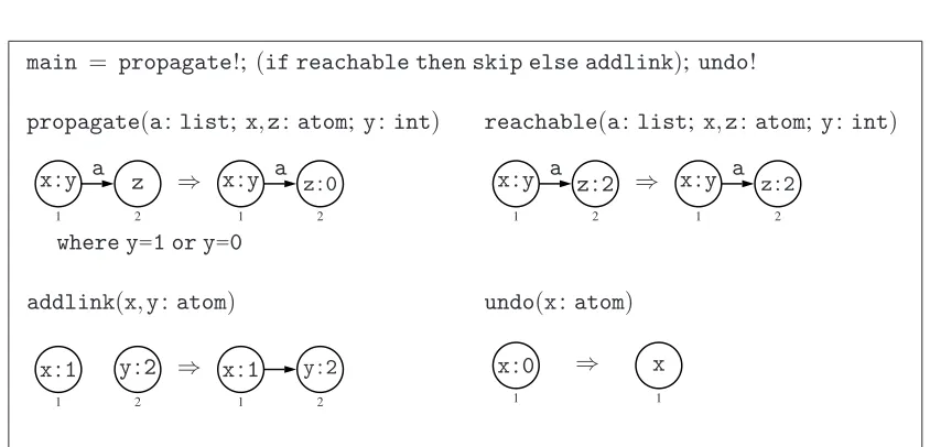
The program reachable? in Figure 4 checks whether or not there is a path from one dis-tinguished node (tagged with 1) to another (tagged with 2), again provided that the input graph contains unmarked items only and the list components of nodes are atoms (except for the distin-guished nodes). An execution ofreachable? returns the original input graph if there exists such a path, otherwise it returns the same graph but with an additional edge linking the distinguished nodes. Withpropagate!, the program iteratively tags nodes with 0 that are reachable from the 1-tagged node. An if-then-else conditional is then encountered: if its “guard”reachable can be applied (to a copy of the graph), thenskipis executed; otherwiseaddlink. The idea is as follows: ifreachablecan be applied, then there must be a tagged node adjacent to the second distinguished node, indicating the existence of a path. In this case,skip is applied which does not change the graph. Ifreachablecannot be applied, then there must not exist a path, and so addlinkis applied to add an edge directly between the distinguished nodes. In both cases, the 0-tags used in the computation are removed by the iteration ofundo.
main= init!;inc!
init(x:atom) inc(i:int;k:list; x,y:atom)
1
x ⇒
1
x:0 x:i y:i
1 2
k ⇒
x:i y:i+1
1
2
k
3
3
3 3
3 3
3
3 ⇒+ 3:0
3:1
3:0 3:1
3 3
3 3
⇒+
3:0
3:1
3:2 3:1
3 3
3 3
Figure 3: The programcolouringand two of its executions
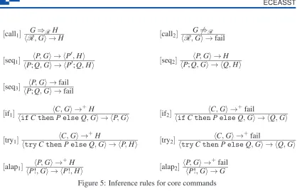
The formal semantics of GP is given in the style of structural operational semantics. Inference rules inductively define a small-step transition relation→ on configurations. In our setting, a configuration is either a command sequence (ComSeq) together with a graph (i.e. an unfinished computation), just a graph, or the special element fail (representing a failure state). The meaning of graph programs is summarised by a semantic function J K, which assigns to every program Pthe functionJPKmapping an input graphGto the set of all possible results of runningPon G. The result set may contain, besides proper results in the form of graphs, the special values fail and⊥. The value fail indicates a failed program run whilst⊥indicates a non-terminating or stuck computation. Thesemantic functionJ K: ComSeq→(G(L)→2G(L)∪{fail,⊥})is defined by:
JPKG={X∈(G(L)∪ {fail})| hP,Gi→+ X} ∪ {⊥ |Pcan diverge or get stuck fromG} whereP can diverge from Gif there is an infinite sequencehP,Gi → hP1,G1i → hP2,G2i →. . ., andP can get stuck from Gif there is a terminal configurationhQ,Hisuch thathP,Gi →∗hQ,Hi
where the rest programQcannot be executed because no inference rule is applicable. A program can get stuck if it contains a non-terminating subprogram in a loop or in a conditional.
Figure 5shows the inference rules of commands in GP 2. Each rule consists of a premise and a conclusion separated by a horizontal bar. Both parts contain meta-variables for command sequences and graphs, whereR stands for a rule schema set call,C,P,P′,Qstand for command sequences, andG,Hstand for graphs inG(L). Meta-variables are considered to be universally quantified. The notationG6⇒R expresses that for graphGinG(L)there is no graph H such
main = propagate!; (if reachable then skip else addlink);undo!
propagate(a:list;x,z:atom;y:int) reachable(a:list; x,z:atom; y:int) x:y z
1 2
a
⇒ x:y z:0
1 2
a
x:y z:2
1 2
a
⇒ x:y z:2
1 2
a
where y=1 or y=0
addlink(x,y:atom) undo(x:atom)
x:1 y:2
1 2
⇒ x:1 y:2
1 2 1
x:0 ⇒
1
x
Figure 4: The programreachable?
programs made up of core commands only (in this case, the rule schema /0⇒ /0). We refer to [Plu12] for details.
4
Proving Partial Correctness
In this section we first review E-conditions, the assertion language of our proof calculi. Then, we review the partial correctness proof calculus presented in previous work (updated for GP 2, e.g. the new [try] proof rule).
Nested graph conditions with expressions(orE-conditions) are a morphism-based formalism for expressing both structural properties of graphs and properties about their labels. E-conditions [PP12a] extend the nested conditions of [HPR06] with expressions for labels and assignment constraints, which are simple Boolean expressions used to restrict the instantiations of variables to values of particular types, or values that hold in particular relations. A simple example of an E-condition is:
¬∃( x |int(x))
which is satisfied by graphs that do not have any unmarked integer-labelled nodes. The formal-ism combines logical quantifiers with graph structure and constraints on labels: E-conditions demand the (non-)existence of particular subgraphs, subject to some constraint on the labels (the vertical bar can be read as “such that”). More generally, the formalism exploits nesting to allow universally quantified expressions. For example,
∀( x
1|atom(x),∃( x 1)∨ ∃( x 1))
[call1] G⇒RH
hR,Gi →H [call2]
G6⇒R
hR,Gi →fail
[seq1] hP,Gi → hP′,Hi
hP;Q,Gi → hP′;Q,Hi [seq2]
hP,Gi →H hP;Q,Gi → hQ,Hi
[seq3]hPhP;Q,G,Gi →i →failfail
[if1] hC,Gi →
+H
hifCthenPelseQ,Gi → hP,Gi [if2]
hC,Gi →+fail
hifCthenPelseQ,Gi → hQ,Gi
[try1] hC,Gi →
+H
htryCthenPelseQ,Gi → hP,Hi [try2] hC,Gi → +fail
htryCthenPelseQ,Gi → hQ,Gi
[alap1] hP,Gi →
+H
hP!,Gi → hP!,Hi [alap2] hP,Gi → +fail hP!,Gi →G Figure 5: Inference rules for core commands
identifies the nodes as being the same; the nesting adds more detail about the required context of the particular subgraph.
Similarly to rule schemata, in checking whether a graph satisfies a property described by an E-condition, a suitable assignment α must be found for the label expressions and assignment constraint. Note however that unlike in rule schemata, we are not declaring types for variables, but rather using predicates about types within assignment constraints. For example, we could writenot int(x)as an assignment constraint, or even omit type predicates completely.
Due to space limitations we do not give a formal syntax or semantics of assignment constraints (we refer the reader to [PP12a, Pos13]) – there are several examples in this paper however. Example1includes a simple assignment constraint,x>y. An assignment is well-typed for this if it maps bothxandyto integers. Such an assignment constraintγis evaluated with respect to a well-typed assignmentα, denotedγα, by instantiating variables with the values given byα and then replacing function and relation symbols with the obvious functions and relations.
In our formal definition of E-conditions, the part of the formalism immediately after each quantifier is a morphism – not simply a graph. In our examples, we draw only the codomains; in general there are chains of morphisms along the nesting (starting from the empty graph in this paper). We discuss this aspect of E-conditions in more detail shortly.
In order to define the satisfaction relation for E-conditions, we first define substitutions to allow the replacement of variables with lists (this is used to enforce equal assignment of variables in the nesting of E-conditions). Asubstitutionis a partial functionσ: VarId→List. Given a label (e b)withea list andba mark,σiswell-typedforeif it does not replace variables in arithmetic (resp. string) expressions with string (resp. arithmetic) expressions. In this case, the list eσ is obtained from e by replacing every variable x for which σ is defined with σ(x) (if σ is not defined for a variablex, thenxσ =x). Given a graphGinG(Label)such thatσ is well-typed for all lists inG, we writeGσ for the graph inG(Label)that is obtained by replacing each list ewitheσ. Ifg:G→H is a graph morphism between graphs inG(Label), thengσ denotes the morphismhgV,gEi:Gσ →Hσ. A substitutionσ: VarId→List can be applied to an assignment
constraintγ, if it is well-typed for all expressions in γ. The resulting assignment constraint, denoted byγσ, is simplyγ with each expressionereplaced byeσ.
Given an assignment α: VarId→L, thesubstitution σα: VarId→List induced byα maps
every variablexto the expression that is obtained fromα(x)by replacing integers and strings with their syntactic counterparts. For example, ifα(x)is the integer 23, thenσα(x)is23(the syntactic digits). Consider another example: ifα(x)is the sequence 56 : “a” : “bc” , where 56 is an integer and “a” and “bc” are strings, thenσα(x) =56: ”a” : ”bc”.
The satisfaction of E-conditions by injective graph morphisms between graphs in G(L) is defined inductively. Every such morphism satisfies the E-conditiontrue. An injective graph morphisms:S֒→GwithS,G∈G(L)satisfiesthe E-conditionc=∃(a:P֒→C|γ,c′), denoted s|=c, if there exists an assignmentαthat is well-typed for all expressions inP,C,γand is unde-fined for variables present only inc′, such thatS=Pα, and such that there is an injective graph morphismq:Cα֒→Gwithq◦aα=s,γα =true, andq|= (c′)σα. Here, σα is the substitution induced byα, which we require to be well-typed for all expressions inc′. If such an assignment α and morphism qexist, we say that s satisfies c byα, and writes|=αc. The satisfaction of Boolean formulae over E-conditions is defined inductively, in the obvious way.
For brevity, we writefalsefor¬true,∃(a|γ)for∃(a|γ,true),∃(a,c′)for∃(a|true,c′), and∀(a|γ,c′)for¬∃(a|γ,¬c′). In our examples, when the domain of morphisma:P֒→Ccan unambiguously be inferred, we write only the codomainC. For instance, an E-condition∃(/0֒→ C,∃(C֒→C′))can be written as∃(C,∃(C′)), where the domain of the outermost morphism is the empty graph, and the domain of the nested morphism is the codomain of the encapsulating E-condition’s morphism.
An E-condition over a graph morphism whose domain is the empty graph is referred to as an E-constraint.
Example 1 The E-constraint∀( x y
1 2 k
|x>y,∃( x y
1 2 l
k
))expresses that every pair of unmarked integer-labelled nodes linked by an unmarked edge with the source label greater than the target label, has an unmarked loop incident to the source node. The (fully) unabbreviated version of the E-constraint is as follows:
¬∃(/0֒→ x
1
y
2 k
|x>y,¬∃( x
1 2
y
k
֒→
1
x
2
y
l k
|true,true)).
Definition 2 (Partial correctness) A graph program P is partially correct with respect to a preconditioncand postconditiond (both of which are E-constraints), denoted|=par{c}P{d}, if for every graphG∈G(L),G|=cimpliesH|=dfor every graphHinJPKG.
In [PP12a] we defined axioms and inference rules for proving partial correctness specifications about graph programs. These are given in Figure6(with [try] new for GP 2), wherer(resp.R) ranges over conditional rule schemata (resp. sets of conditional rule schemata),c,c′,d,d′,e,inv over E-constraints, andP,Qover graph programs. Together, the axioms and rules define a proof system for partial correctness. If a Hoare triple {c} P{d}can be proved via the axioms and inference rules (by constructing a proof tree, as in Section6), we write⊢par{c}P{d}. The proof system is sound in the sense of partial correctness, that is,⊢par{c}P{d}implies|=par{c}P{d} (see [PP12a] for GP 1, and [Pos13] for an analogous GP 2 proof).
[ruleapp]
{Pre(r,c)}r{c} [nonapp] {¬App(R)}R{false}
{c}r{d}for eachr∈R [ruleset]
{c}R{d}
{inv}R{inv} [!]
{inv}R!{inv∧ ¬App(R)}
{c}P{e}, {e}Q{d} [comp]
{c}P;Q{d}
c⇒c′, {c′}P{d′}, d′⇒d [cons]
{c}P{d}
{c∧App(R)}P{d}, {c∧ ¬App(R)}Q{d} [if]
{c}ifRthenPelseQ{d}
{c∧App(R)}R;P{d}, {c∧ ¬App(R)}Q{d} [try]
{c}tryRthenPelseQ{d}
Figure 6: Partial correctness proof rules for core commands
Two transformations – App and Pre – appear in the axioms and rules. Intuitively, App takes as input a setR of conditional rule schemata, and transforms it into an E-condition satisfied only by graphs for which at least one rule schema inRis applicable. Pre on the other hand constructs an E-condition such that ifG|=Pre(r,c), and the application ofrtoGresults in a graphH, then H|=c. Formal constructions of the transformations are omitted from this paper, but can be found in [PP12a] for GP 1 (and for GP 2, in [Pos13]).
pro-grams). Without this restriction, the proof rules would require an assertion language able to express that an arbitrary program will not fail.
5
Proving Total Correctness
If ⊢par {c} P {d}, then if P is executed on a graph G satisfying c, we can be sure that any graph resulting will satisfyd. What we cannot be sure about is whether an execution ofPwill ever terminate (i.e. whether an execution might diverge or not). Moreover, if an execution ofP does in fact terminate, we cannot be sure that it does so without failure. When referring tototal correctness, we follow [Apt84] in meaning both absence of divergence and failure; and when referring toweak total correctness, we mean only absence of divergence.
Definition 3 (Weak total correctness) A graph program P isweakly totally correct with re-spect to a preconditioncand postconditiond (both of which are E-constraints), denoted|=wtot {c} P {d}, if |=par {c} P {d} and for every graph G∈G(L) such that G|=c, we have ⊥∈/JPKG.
Definition 4 (Total correctness) A graph programP is totally correct with respect to a pre-conditionc and postconditiond (both of which are E-constraints), denoted|=tot{c}P{d}, if |=wtot{c}P{d}, and for every graphG∈G(L)such thatG|=c, we have fail∈/JPKG.
A weakly totally correct program executed on a graph satisfying the precondition will either produce an output graph or terminate with failure (it cannot diverge or get stuck). A totally correct program however has the additional guarantee that it will not fail, that is, a graph will eventually result from its execution.
Our proof system for weak total correctness is formed from the proof rules of Figure6, but with [!]tot in Figure7substituted for [!]. If a triple{c}P{d}can be obtained from this proof system, we write⊢wtot{c}P{d}. The issue of termination is localised to the proof rule for as-long-as-possible iteration: [!]tothas an additional premise to [!] which handles this. It requires, for a given rule schema set, that there is a function assigning natural numbers to graphs such that these naturals are decreasing along rule applications. Such a function # is called atermination function. If the #-values of graphs satisfying the invariantinvdecrease under applications ofR, we say thatRis #-decreasing under inv. These definitions are given more precisely below.
⊢par{inv}R{inv}, Ris #-decreasing underinv [!]tot
{inv}R!{inv∧ ¬App(R)}
c⇒App(R), ⊢par{c}r{d}for eachr∈R [ruleset]tot
{c}R{d}
Definition 5 (Termination function; #-decreasing) A termination function is a mapping # : G(L)→Nfrom (semantic) graphs to natural numbers. Given an E-constraintc, a set of
condi-tional rule schemataR is #-decreasing under cif for all graphsG,HinG(L)withG|=cand H|=c,
G⇒RHimplies #G>#H.
In an application of [!]tot, one must find a suitable termination function # that returns smaller natural numbers along the graphs of direct derivations. The problem of deciding whether a set of rule schemata has a termination function or not is undecidable in general [Plu98]. Often however simple termination functions will suffice in several contexts. For example, a useful, intuitive termination function would be one that maps a graph to its size (e.g. total number of nodes and edges). If a rule schemata set is reducing the size of a graph upon each application, then clearly the iteration cannot continue indefinitely, and this is reflected by the output of # tending towards zero. However, in cases when rule schemata are not decreasing the size of the graph, less obvious termination functions may be needed (one such example will be discussed in Section6). Note that the rule [!]totrequires only that # is decreasing for graphs that satisfy the invariantinv, i.e. it need not be decreasing for other graphs.
Our proof system for total correctness is formed of [comp], [cons], [if], [try], and the proof rules of Figure 7. If a triple {c} P {d} can be derived from this proof system, we write ⊢tot{c}P{d}. (We do not include a proof rule for a program that is just a single rule schema r, because this case is captured by proving⊢tot{c} {r} {d}.) This proof system allows one to prove that all program executions terminate without failure. Essentially, this is achieved by en-suring that the preconditions of rule schema sets imply their applicability, when they are applied outside of iterations or the guards of conditionals. Hence if graphs satisfy the preconditions, by implication the rule schema sets are applicable to those graphs, and thus we can be certain that no execution will fail.
The proof rule [ruleset]totseparates the issues of failure and partial correctness. In using the proof rule, one must show (outside the calculus) that the applicability ofRis logically implied by the preconditionc. In showing that this premise holds, we can be sure that at least one rule schema inR can be applied to a graph satisfyingc, hence no execution on that graph will fail. Separately, it must be shown that⊢par{c}r{d}for eachr∈R, that is, each rule schema in the set is partially correct with respect to the pre- and postcondition. Together, we derive that every execution ofRwill yield a graph, and that the graph will satisfy the postcondition.
The axiom [nonapp] is excluded from our proof system for total correctness, as the specifica-tion{¬App(R)}R{false}does not hold in the sense of total correctness. Suppose that it did. ThenRwould never fail on graphs satisfying the precondition. But satisfying¬App(R)implies thatRfails on that graph – a contradiction.
6
Example Proofs
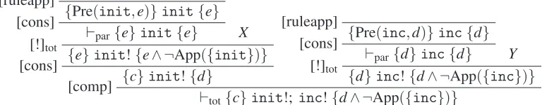
First, we revisit the programcolouringof Figure3. Though the program contains no failure points (since if a rule schema under as-long-as-possible iteration cannot be applied, the execution simply moves on to the next command), the iteration operator can introduce non-termination. In [PP12a] we proved that colouringis partially correct, in the sense that any graph resulting is properly coloured. In Figure8, we strengthen this to⊢tot{c}colouring{d∧ ¬App({inc})}, i.e. if the program is executed on a graph containing only atom-labelled nodes, then (1) a graph will eventually be returned; (2) it will be properly coloured; and (3) for any colournin the graph, every colourkwith 0≤k<nis also in the graph. (The specification ignores marked nodes and edges for simplicity.) Note that the E-conditions resulting from Pre, implications in instances of [cons], and their justifications, are omitted to preserve space – but can be found in [Pos13].
[ruleapp]
{Pre(init,e)}init{e} [cons]
⊢par{e}init{e} X [!]tot
{e}init!{e∧ ¬App({init})} [cons]
{c}init!{d}
[ruleapp]
{Pre(inc,d)}inc{d} [cons]
⊢par{d}inc{d} Y [!]tot
{d}inc!{d∧ ¬App({inc})} [comp]
⊢tot{c}init!; inc!{d∧ ¬App({inc})} X :initis #init-decreasing undere; Y :incis #inc-decreasing underd
c = ∀( a
1,∃( a1|atom(a)))
d = ∀( a
1,∃( a1|a=b:c and atom(b)and c>=0))
∧ ∀(b:c
1|atom(b),∃(b:c1|c=0)
∨ ∃(b:c 1
d:c-1 |atom(d)))
e = ∀( a
1,∃( a1|atom(a))
∨ ∃( a
1|a=b:c and atom(b)and c>=0))
∧ ∀(b:c
1|atom(b),∃(b:c1|c=0)
∨ ∃(b:c
1 d:c-1 |atom(d)))
¬App({init}) = ¬∃( x |atom(x))
¬App({inc}) = ¬∃(x:i k y:i |atom(x,y)and int(i))
Figure 8: A proof tree for the programcolouringof Figure3
The key revision in the proof tree is in the two uses of [!]tot, which unlike its partial correctness counterpart requires the definition of termination functions. Forinit, we define #init:G(L)→ Nto map graphs to the number of their nodes labelled by an atom. The rule schema is clearly
#init-decreasing under e, since every application ofinitreduces by one the number of nodes
#inc:G(L)→N. For a graphG∈G(L), we define:
#inc(G) = |VG|
∑
i=0i−
∑
v∈VG
colour(v)
where colour(v)for a nodev∈VGis defined:
colour(v) =
i iflG(v) =x:iwithx∈Z∪Char∗,i∈N;
0 otherwise.
We show thatincis #inc-decreasing underinv. Observe that ifGis a graph with colour(v) =0
for every nodevinVG, then for every derivationG⇒∗incHthere is some 0≤k<|VH|such that
kis the largest tag inVH. We obtain an upper bound for the second summation:
∑
v∈VHcolour(v)≤0+1+· · ·+ (|VH| −1) =0+1+· · ·+ (|VG| −1)< |VG|
∑
i=0 i.Since ∑v∈VHcolour(v) equals the number of rule schema applications in G⇒∗incH, it
fol-lows thatincmust eventually terminate (as it approaches the upper bound). By subtracting the summation from the upper bound, we instead have a number decreasing towards 0 after every application ofinc. Hence #inc is a suitable termination function, and incis #inc-decreasing
underinv.
We remark thatinc! will terminate on any graph – not just those satisfyinginv. A termination function however is harder to write without the assumptions the invariant allows us to make about the graphs.
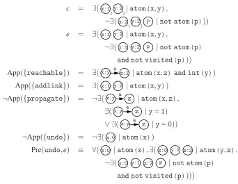
Now, we return to the programreachable? of Figure4, which unlike earlier, can fail on some input graphs (in particular, those graphs omitting the pair of 1- and 2-tagged nodes). We give a proof tree3for⊢tot{c}reachable?{c}in Figure9, where the E-constraints are as in Figure10. For clarity, we letvisited(p)abbreviate:
p=a:0 and atom(a) whereais a fresh variable.
If the program is executed on a graph that contains only atom-labelled nodes but with one tagged 1 and another tagged 2, then (1) the program is guaranteed to return a graph eventually; and (2) that graph will satisfy the same condition (i.e. an invariant). Again, due to space limita-tions, we have omitted the implications in instances of [cons] and their justifications. Moreover, we have only provided one of the E-constraints generated by Pre.
In this proof tree, there are simple suitable termination functions #p,#u. We define the
ter-mination function #p:G(L)→N(resp. #u) to return the number of nodes in a graph that are
labelled by an atom (resp. number of atom-labelled nodes tagged with a 0). That is, both termi-nation functions exploit that each application of their respective rule schema explicitly reduces the number of remaining matches.
3For simplicity we use an obvious additional axiom [skip]:⊢
V e ri fy in g T o ta l C o rr e c tn e s s o f G ra p h P ro g ra m s
LetP=if reachable then skip else addlink
[ruleapp]
{Pre(propagate,e)}propagate{e}
[cons]
⊢par{e}propagate{e} propagateis #p-decreasing undere
[!]tot
{e}propagate!{e∧ ¬App({propagate})}
[cons]
{c}propagate!{e} SubtreeX
[comp]
⊢tot{c}propagate!;P;undo!{c}
SubtreeX:
[skip]
{e}skip{e}
[cons]
{e∧App({reachable})}skip{e} SubtreeY
[if]
{e}P{e}
[ruleapp]
{Pre(undo,e)}undo{e}
[cons]
⊢par{e}undo{e} undois #u-decreasing undere
[!]tot
{e}undo!{e∧ ¬App({undo})}
[cons]
{e}undo!{c}
[comp]
{e}P; undo!{c}
SubtreeY:
e∧ ¬App({reachable})⇒App({addlink})
[ruleapp]
{Pre(addlink,e)}addlink{e}
[cons]
⊢par{e∧ ¬App({reachable}}addlink{e}
[ruleset]tot
{e∧ ¬App({reachable})}addlink{e}
Figure 9: Total correctness proof tree for the programreachable? of Figure4
c = ∃(x:1 1
y:2
2|atom(x,y),
¬∃(x:1 1
y:2 2
p |not atom(p)))
e = ∃(x:1 y:2 |atom(x,y),
¬∃(x:1 y:2 p |not atom(p)
and not visited(p)))
App({reachable}) = ∃(x:y a z:2 |atom(x,z)and int(y)) App({addlink}) = ∃(x:1 y:2 |atom(x,y))
¬App({propagate}) = ¬∃(x:y a z |atom(x,z),
∃(x:y a z |y=1)
∨ ∃(x:y a z |y=0))
¬App({undo}) = ¬∃(x:0 |atom(x))
Pre(undo,e) ≡ ∀(x:0 |atom(x),∃(x:0 y:1 z:2 |atom(y,z), ¬∃(x:0 y:1 z:2 p |not atom(p)
and not visited(p))))
Figure 10: Partial list of E-constraints for Figure9
The rule schemaaddlinkis the only potential failure point of the program, and is addressed in the proof tree by the application of [ruleset]tot. It must be shown that the precondition at that point implies the applicability ofaddlink. From Figure10, it is clear that satisfyinge is sufficient to deduce the applicability ofaddlink.
7
Soundness and Completeness for Termination
In this section we revise our soundness proof from [PP12a] to account for (weak) total correct-ness, before showing that any iterating rule schemata set that terminates can be proven to ter-minate by the rule [!]tot. Soundness is relative to the operational semantics of the language. An updated version of the soundness proof for partial correctness with regards to the GP 2 semantics can be found in [Pos13].
Theorem 1(Soundness of⊢wtot) For all graph programsPand E-constraintsc,d, we have that ⊢wtot{c}P{d}implies|=wtot{c}P{d}.
Proof. For all weak total correctness proof rules except [!]tot, this follows from (1) the soundness result for partial correctness in [PP12a], and (2) the semantics of graph programs, from which it is clear that only as-long-as-possible iteration can introduce divergence.
G,H∈G(L)withG|=invandH|=inv,G⇒R Himplies #G>#H. Assume thatR! diverges for any suchG. SinceRis #-decreasing underinv, every derivation step yields a graph for which # returns a smaller natural number. SinceR! diverges, there are infinitely many derivation steps. But from any naturaln, there are only finitely many smaller numbers. A contradiction. It cannot be the case thatR! diverges from any suchG. Hence|=wtot{inv}R!{inv∧ ¬App(R)}.
Theorem 2(Soundness of⊢tot) For all graph programsPand E-constraintsc,d, we have that ⊢tot{c}P{d}implies|=tot{c}P{d}.
Proof. For the proof rules [comp], [cons], [if], [try], [!]tot, this follows from (1) the soundness of⊢wtot (see Theorem1), and (2) the semantics of graph programs, from which it is clear that these proof rules are sound in the sense of total correctness. What remains to be shown is the soundness of [ruleset]totin the sense of total correctness.
Let R denote a set of (conditional) rule schemata and c,d denote E-constraints. Assume that⊢par{c} r {d} for eachr∈R. Then by soundness for partial correctness, we have |=par {c}R{d}. Now assume the validity ofc⇒App(R). Then if a graphG∈G(L)satisfiesc, by assumption it will satisfy App(R). By Proposition 7.1 of [PP12a] (updated for the GP 2 syntax in [Pos13]), there is a graphHsuch thatG⇒RH. Then the semantic rule [call1] will be applied
(and in particular, [call2] will not be), hence a graph is guaranteed from the execution and failure is avoided. We yield|=tot{c}R{d}.
Now, we show that every iterating set of rule schemata that terminates can be proven to ter-minate using [!]tot, by showing that there always exists a termination function for which the rule schemata set is decreasing under its invariant.
Theorem 3(Completeness of[!]totfor termination) LetRbe a set of conditional rule schemata andcbe an E-constraint such that for every graphGinG(L), G|=cimplies thatR! cannot diverge fromG. Then there exists a termination function # such thatR is #-decreasing under c.
Proof. LetGbe a graph such thatG|=c. Then there cannot exist an infinite sequenceG⇒R G1⇒R G2⇒R . . . as otherwise, by the semantics of GP, there would be an infinite sequence
hR!,Gi → hR!,G1i → hR!,G2i. . .. To define the termination function #, we show that the length of ⇒R-derivations starting from G is bounded. (Note that, in general, a terminating
relation need not be bounded.)
We exploit that⇒Ris closed under isomorphism in the following sense: given graphsM,M′,N
andN′such thatM∼=M′andN∼=N′, thenM⇒RNimpliesM′⇒RN′. Hence we can lift⇒R
to a relation on isomorphism classes of graphs by defining:[M]⇒R[N]ifM⇒RN. Then, since
Ris finite, for every isomorphism class[M]the set{[N]|[M]⇒R [N]}is finite.
Now, since there is no infinite sequence of⇒R-steps starting from[G], it follows from K¨onig’s
lemma [K¨on36] that the length of⇒R-derivations starting from[G]is bounded. (In the tree of all
derivations starting from[G], all nodes have a finite degree. Hence the tree cannot be infinite, as otherwise it would contain an infinite derivation.) Hence the length of⇒R-derivations starting
M⇒RN, we have #M>#N. ThusRis #-decreasing underc.
8
Conclusion
In this paper we have presented two Hoare calculi which allow one to prove (weak) total correct-ness. Both proof systems have been shown to be sound. We have shown how to reason about termination via termination functions, and shown that the proof rule for termination is complete in the sense that all terminating loops (having a set of conditional rule schemata as the body) can be proven to be terminating. Finally, we have demonstrated the use of the proof systems on two non-trivial graph programs, showing how to prove the absence of divergence and failure.
Future work will explore how to implement the proof calculi in an interactive proof system. A first step towards this is made in [Pos13], in which translations from E-conditions to many-sorted formulae (and back) are defined, providing a suitable front-end logic for an implemented verification system. Future work will also address the question of whether or not the calculi are (relatively) complete. It would also be worthwhile to integrate a stronger assertion language into the calculi that can express non-local properties, such as the hyperedge-replacement conditions of [HR10].
Acknowledgements: We thank the anonymous referees for their comments which helped to improve the final version of this paper. Most of this work was completed whilst the first author was a Ph.D. student at the University of York, where he was supported by a scholarship of the Engineering and Physical Sciences Research Council. Since January 2013 he has been based at ETH Z¨urich, where he is supported with funding from the European Research Council (ERC grant agreement no. 291389).
Bibliography
[Apt84] K. R. Apt. Ten Years of Hoare’s Logic: A Survey Part II: Nondeterminism.Theoretical Computer Science28:83–109, 1984.
[BCK08] P. Baldan, A. Corradini, B. K¨onig. A framework for the verification of infinite-state graph transformation systems.Information and Computation206(7):869–907, 2008. [BHE09] D. Bisztray, R. Heckel, H. Ehrig. Compositional Verification of Architectural
Refac-torings. InProc. Architecting Dependable Systems VI (WADS 2008). Volume 5835, pp. 308–333. Springer-Verlag, 2009.
[CR12] S. A. da Costa, L. Ribeiro. Verification of graph grammars using a logical approach. Science of Computer Programming77(4):480–504, 2012.
[HP09] A. Habel, K.-H. Pennemann. Correctness of high-level transformation systems relative to nested conditions. Mathematical Structures in Computer Science19(2):245–296, 2009.
[HPR06] A. Habel, K.-H. Pennemann, A. Rensink. Weakest Preconditions for High-Level Pro-grams. InProc. International Conference on Graph Transformation (ICGT 2006). Vol-ume 4178, pp. 445–460. Springer-Verlag, 2006.
[HR10] A. Habel, H. Radke. Expressiveness of graph conditions with variables. InProc. Col-loquium on Graph and Model Transformation on the Occasion of the 65th Birthday of Hartmut Ehrig. Electronic Communications of the EASST 30. 2010.
[KE10] B. K¨onig, J. Esparza. Verification of Graph Transformation Systems with Context-Free Specifications. In Proc. International Conference on Graph Transformation (ICGT 2010). Volume 6372, pp. 107–122. Springer-Verlag, 2010.
[K¨on36] D. K¨onig. Sur les correspondances multivoques des ensembles.Fundamenta Mathe-maticae8:114–134, 1936.
[Plu98] D. Plump. Termination of Graph Rewriting is Undecidable.Fundamenta Informaticae 33(2):201–209, 1998.
[Plu09] D. Plump. The Graph Programming Language GP. In Proc. Algebraic Informatics (CAI 2009). Volume 5725, pp. 99–122. Springer-Verlag, 2009.
[Plu12] D. Plump. The Design of GP 2. InProc. International Workshop on Reduction Strate-gies in Rewriting and Programming (WRS 2011). Electronic Proceedings in Theoreti-cal Computer Science 82, pp. 1–16. 2012.
[Pos13] C. M. Poskitt.Verification of Graph Programs. PhD thesis, The University of York, 2013. To appear.
[PP12a] C. M. Poskitt, D. Plump. Hoare-Style Verification of Graph Programs.Fundamenta Informaticae118(1-2):135–175, 2012.