Vol 9, No 3 (2018)

(1)

International Journal of Mathematical Archive-9(3), 2018,

17-23

Available online throug

ISSN 2229 – 5046A

A STUDY ON (M/M/1): (N/FCFS) QUEUEING MODEL

UNDER MONTE CARLO SIMULATION IN A MULTI SPECIALITY HOSPITAL

S. SHANMUGASUNDARAM

1

_{AND P. UMARANI}

2

1_{Department of Mathematics,}

Government Arts college, Salem – 7, Tamil Nadu, India.

2_{Department of Mathematics,}

AVS Engineering college, Salem – 3, Tamil Nadu, India.

E-mail: [email protected]1 _{and [email protected]}2_.

ABSTRACT

I

n this study, we analyse the queueing model under single server, the system capacity is limited to N. The arrival and service data are collected in a multi speciality hospital in two cases i.e., inpatients and emergency patients. Chi-square test is used for test the goodness of fit in arrival and service distribution. Monte Carlo Simulation method is used to analyse the queue length. We compare the Simulation result with analytical.

Keywords: Arrival, Service, System Capacity, (M/M/1):(N/FCFS) queueing model, Monte Carlo Simulation, Queue

length, Chi-square test.

1. INTRODUCTION

Queues or waiting lines are very common in everyday life. Customers arrive at service counters and are attended by one or more of the servers and the customers leave the system after the service. The service starts from the first person or a thing in the sequence. Analysing and providing the service, servers related to the queue is defined as Queueing theory. Now it can be explained briefly about the topics viz: i) Queuing Theory, ii) Simulation Method, iii) Analytical Method and iv) Chi – Square Test. Queueing theory has originated in the research by Agner Krarup Erlang (1878-1929) a Danish Engineer cum mathematician while creating models to describe the telephone exchange and that was the first paper published which is now called as queueing theory [3]. Characteristics of queueing system are (i) Arrival pattern (ii) Service pattern (iii) Queue discipline (iv) System capacity (v) Number of service channels and (vi) Number of service phases.

M/M/1 QUEUING MODEL

(2)

Chi-square test is used to test the suitability of a distribution and the independence of the attributes. It is used to test the significance of the difference between the observed frequencies in a sample and expected frequencies obtained from the theoretical distribution. Karl Pearson developed a test for testing the significance of discrepancy between experimental values and the theoretical values obtained under some hypothesis. This is

χ

2 test fitness. The test statistic is given by

χ

2_{= ∑} (𝑂𝑖−𝐸𝑖)2

𝐸𝑖

𝑘

𝑖=1 where Oi is the observed frequency in the ith class interval and Ei is the expected frequency in that

class interval. The expected frequency for each class interval is computed as E i is the npi where pi is the theoretical,

hypothesized probability associated with the ith class interval.

The aims of this paper are i) to check the goodness-of-fit of arrival and service distribution, and ii) to determine the queue length both in Simulation and Analytical method.

Ishan, P. Lade, Sandeep, A. Chowriwar and Pranay, B. Sawaitul (2013) have described the use of queueing systems to decrease the waiting time of patients in the queueing system using simulation method [5]. Shanmugasundaram, S. and Punitha, S., (2014) has analyzed the application of simulation in queueing model in tollgate [8]. Syed Shujauddin Sameer (2014) has helped in understanding the behaviour of a queueing system using simulation and also obtains certain very useful parameters. In this paper, simulation provides a good strategy to analyze the client – server systems and to solve the complicated problems. One of the important applications of the Simulation is the analysis of the waiting line problem and it is classified into Deterministic Model, Probabilistic Model, Static Model and Dynamic Model [12]. Shanmugasundaram, S. and Banumathi, P. (2016) have aimed to reduce the queue length, system length, queue time and system time in Southern railway using simulation in queueing analysis. Simulation is a mimic of reality that exists or which is contemplated. Simulation is most effectively used as a queueing analysis [7]. Soemon Takakuwa and Athula Wijewickrama (2008) have described the application of the simulation for patients coming to the hospital, the pertinent parameters like waiting time, service time, waiting time and service time ratio [11]. Shanmugasundaram, S. and Umarani, P., (2016) have discussed the applications of simulation in queueing model at a medical center and how to calculate the queue time, system time, queue length and system length in the Simulation table [10]. They (2016) also have analyzed the queueing system in a simulation model of a medical center in order to develop an efficient procedure for reducing the waiting time of the patients in the queue [9]. Ishan, P. Lade, V. P. Sakhare, M. S. Shelke and P. B. Sawaitul (2015) have analyzed the applications of queueing model using Simulation and to reduce the average waiting time of patients for chemotherapy section in the radiation therapy and oncology department [6]. Gateri Judy Muthoni, Stephen Kimani, Joseph wafula (2014) have compared the existing prediction models and come up with Monte Carlo Simulation model to predict the number of patients in the queue [4]. Alireza Saremi, Payman Jula, Tarek ElMekkawy, G. GaryWang (2012) have addressed the appointment scheduling of outpatient surgeries in a multistage operating room department with stochastic service times serving multiple patient types and have described to minimize the patients wait time and patients completion time by using Simulation-based optimization method [1].

2. DESCRIPTION OF THE MODEL

Initially, the arrival data of inpatients (Admitted patients) and emergency patients in a multi speciality hospital has been collected for a week, during the month of September 2017. Every department in a hospital has been assigned with a specialist for Inpatients and emergency patients. The actual queue length of the patients at the hospital is calculated through Monte Carlo Simulation and Analytical methods with (M/M/1) : (N/FCFS). The results of both the models were identical and they are illustrated in Table 11. As the objective of this paper is to minimize or nullify the queue length of the patients, Chi – Square test was used to check whether the arrival and the service of the patients are uniformly distributed. Generally, it is very tiresome for the patients to wait at a hospital as they may be both physically and psychologically weak. Further, patients have to wait for a long time in the queue for their turn which is undesirable. The problem of patients’ waiting in the queue is solved in this paper. The number of patients accommodated in each department (N) is 25.

Table-1: Tag Number Table for Arrival Chosen

S. No. Type of Patients Probability Cumulative Probability Tag numbers

1 In Patients 0.4 0.4 0 – 39

(3)

Table-2: Tag Number Table for Day Choosen

Table-3: Arrival Distributions for in Patients

Table-4: Chi-Square Test for in Patients Arrival

DISTRIBUTION

Null Hypothesis H0: The arrival follows uniform distribution.

The level of significance: 𝛼= 0.01 . Degrees of freedom =7. Calculated value of

χ

2 = 1.392 Tabulated value of

χ

2 for 6 degrees of freedom at 1% level of significance is 16.812. Since

χ

2 <

χ

2₀_.₀₁, It is accepted as 𝐻₀and concluded that the arrival follows the Uniform distribution and it is suitable for the given time of interval.

Table-5: Tag Numbr Table for in Patients Arrival Distribution

S. No. DAY Probability Cumulative probability Tag number

1 MONDAY 0.13 0.13 0 – 12

2 TUESDAY 0.13 0.26 13 – 25

3 WEDNESDAY 0.13 0.39 26 – 38

4 THURSDAY 0.13 0.52 39 – 51

5 FRIDAY 0.17 0.69 52 – 68

6 SATURDAY 0.17 0.86 69 – 85

7 SUNDAY 0.14 1 86 – 100

S.No. DAY No of Patients Probability

1 MONDAY 31 0.16

2 TUESDAY 28 0.14

3 WEDNESDAY 26 0.13

4 THURSDAY 32 0.16

5 FRIDAY 27 0.14

6 SATURDAY 29 0.15

7 SUNDAY 25 0.12

8 TOTAL 198 -

S.NO. DAY

No of Patients

f Ei

χ

2

1 MONDAY 31 28.28 0.26

2 TUESDAY 28 28.28 0.002

3 WEDNESDAY 26 28.28 0.18

4 THURSDAY 32 28.28 0.49

5 FRIDAY 27 28.28 0.06

6 SATURDAY 29 28.28 0.02

7 SUNDAY 25 28.28 0.38

8 TOTAL 198 - 1.392

S. No. DAY No of Patients Probability Cumulative probability Tag number

1 MONDAY 31 0.16 0.16 0 – 15

2 TUESDAY 28 0.14 0.30 16 – 29

3 WEDNESDAY 26 0.13 0.43 30 – 42

4 THURSDAY 32 0.16 0.59 43 – 58

5 FRIDAY 27 0.14 0.73 59 – 72

6 SATURDAY 29 0.15 0.88 73 – 87

7 SUNDAY 25 0.12 1 88 – 100

(4)

Table-6: Arrival Distributions For Emergency Patients

Table-7: Chi-Square Test For Emergency Patients Arrival Distribution

Null Hypothesis H0: The arrival follows uniform distribution.

χ

2 = 3.49. Tabulated value of

χ

2 <

χ

2₀_.₀₁, It is accepted as 𝐻₀and concluded that the arrival follows the Uniform distribution and it is suitable for the given time of interval.

Table-8: Tag Numbr Table For Emergency Patients Arrival Distribution

Table-9: Service Distributions for In and Emergency Patients

S.No. DAY No of Patients Probability

1 MONDAY 33 0.16

2 TUESDAY 25 0.12

3 WEDNESDAY 26 0.12

4 THURSDAY 31 0.15

5 FRIDAY 37 0.18

6 SATURDAY 29 0.14

7 SUNDAY 28 0.13

8 TOTAL 209 -

S.NO. DAY

No of Patients

f Ei

χ

2

1 MONDAY 33 29.85 0.33

2 TUESDAY 25 29.85 0.78

3 WEDNESDAY 26 29.85 0.50

4 THURSDAY 31 29.85 0.04

5 FRIDAY 37 29.85 1.71

6 SATURDAY 29 29.85 0,02

7 SUNDAY 28 29.85 0.11

Total TOTAL 209 - 3.49

S. No. DAY No of Patients Probability Cumulative probability Tag number

1 MONDAY 33 0.16 0.16 0 – 15

2 TUESDAY 25 0.12 0.28 16 – 27

3 WEDNESDAY 26 0.12 0.40 28 – 39

4 THURSDAY 31 0.15 0.55 40 – 54

5 FRIDAY 37 0.18 0.73 55 – 72

6 SATURDAY 29 0.14 0.87 73 – 86

7 SUNDAY 28 0.13 1 87 – 100

8 TOTAL 209 - - -

S. No. DAY No of Patients Probability

1 MONDAY 18 0.13

2 TUESDAY 21 0.15

3 WEDNESDAY 19 0.14

4 THURSDAY 23 0.17

5 FRIDAY 20 0.14

6 SATURDAY 21 0.15

7 SUNDAY 17 0.12

(5)

Table-10: Chi-Square Test For Service Distributions

Null Hypothesis H0: The service follows uniform distribution.

χ

2 = 1.221 Tabulated value of

χ

2 <

χ

2₀_.₀₁, It is accepted as 𝐻₀and concluded that the service follows the Uniform distribution and it is suitable for the given time of interval.

Table-10: Tag Numbr Table For Service Distribution

Table-11: Simulation Table

S. No.

R.No

(DAY) DAY

R.No For Patients

Type of Patients

R.No for

Arrival Arrival

R.No For Service

Service

System capacity

(25)

Queue

1 06 MON 92 EME 43 31 54 23 23 8

2 69 SAT 77 EME 78 29 32 19 19 10

3 85 SAT 81 EME 00 33 86 21 21 12

4 48 THU 13 IN 44 32 40 19 19 13

5 20 TUE 76 EME 79 29 08 18 18 11

6 29 WED 12 IN 72 27 24 21 21 6

7 60 FRI 02 IN 87 29 74 21 21 8

8 07 MON 47 EME 29 26 18 21 21 5

9 26 WED 24 IN 26 28 05 18 18 10

10 30 WED 20 IN 67 27 52 23 23 4

11 18 TUE 44 EME 80 29 54 23 23 6

12 51 THU 82 EME 02 33 32 19 19 14

13 29 WED 14 IN 84 29 86 21 21 8

14 37 WED 59 EME 68 37 40 19 19 18

15 89 SUN 11 IN 11 31 08 18 18 13

16 70 SAT 25 IN 05 31 24 21 21 10

S.NO. DAY

No of Patients

f Ei

χ

2

1 MONDAY 18 19.85 0.17

2 TUESDAY 21 19.85 0.06

3 WEDNESDAY 19 19.85 0.03

4 THURSDAY 23 19.85 0.49

5 FRIDAY 20 19.85 0.001

6 SATURDAY 21 19.85 0.06

7 SUNDAY 17 19.85 0.41

Total TOTAL 139 - 1.221

S.No. DAY No of Patients Probability Cumulative

probability Tag number

1 MONDAY 18 0.13 0.13 0 – 12

2 TUESDAY 21 0.15 0.28 13 – 27

3 WEDNESDAY 19 0.14 0.42 28 – 41

4 THURSDAY 23 0.17 0.59 42 – 58

5 FRIDAY 20 0.14 0.73 59 – 72

6 SATURDAY 21 0.15 0.88 73 – 87

7 SUNDAY 17 0.12 1 88 – 100

(6)

25 62 FRI 47 EME 32 26 81 21 21 5

26 79 SAT 59 EME 35 26 38 19 19 7

27 27 WED 16 IN 25 28 63 20 20 8

28 01 MON 86 EME 92 28 13 21 21 7

29 08 MON 64 EME 17 25 35 19 19 6

30 36 WED 75 EME 15 33 04 18 18 15

31 24 TUE 85 EME 70 37 71 20 20 17

32 84 SAT 82 EME 22 25 40 19 19 6

33 74 SAT 06 IN 08 31 75 20 20 11

34 36 WED 81 EME 33 26 45 23 23 3

35 71 SAT 71 EME 24 25 37 19 19 6

36 61 FRI 52 EME 43 31 47 23 23 8

37 16 TUE 04 IN 66 27 03 18 18 9

38 02 MON 80 EME 38 26 62 20 20 6

39 83 SAT 12 IN 25 28 91 17 17 11

40 83 SAT 69 EME 77 29 71 20 20 9

41 92 SUN 02 IN 44 32 07 18 18 14

42 77 SAT 26 IN 15 31 95 17 17 14

43 81 SAT 56 EME 90 28 03 18 18 10

44 13 TUE 18 IN 77 29 70 20 20 9

45 76 SAT 16 IN 01 31 87 21 21 10

46 12 MON 36 IN 84 29 32 19 19 10

47 02 MON 51 EME 67 37 82 21 21 16

48 47 THU 11 IN 49 32 37 19 19 13

49 27 TUE 62 EME 58 37 86 21 21 16

50 20 TUE 18 IN 89 25 92 17 17 8

1. R.No – RANDOM NUMBER

3. SIMULATION CALCULATION

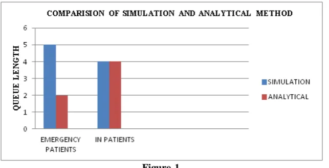
Queue length of emergency patients – 5 Queue length of in patients – 4

4. ANALYTICAL CALCULATION (M/M/1) : (N/FCFS)

Average arrival rate (λ) – 0.03 and Average service rate (μ) – 0.05 Queue length of emergency patients – 2

Queue length of in patients – 4

5. NUMERICAL STUDY

Figure-1

(7)

6. CONCLUSION

In both the cases inpatients and emergency patients, the Simulation result coincides with the Analytical result. Also the bar chart indicates the coincidence.

REFERENCES

1. Alireza Saremi, Payman Jula, Tarek ElMekkawy, G. GaryWang, (2012), “Appointment scheduling of outpatient surgical services in a multistage operating room department”, European Journal of Operational

Research, Elsevier, ISSN:0925-5273.

2. Banks, J., Carson, J.S., Nelson, B.L., and Nicol, D. M., (2001), “Discrete Event System Simulation”, Prentice Hall International Series, Third Edition, 24 - 37.

3. Erlang, A. K., (1909), “The Theory of Probabilities of Telephone Conversations”, Nyt Jindsskriff Mathematic, B20, 33 – 39.

4. Gateri Judy Muthoni, Stephen Kimani, Joseph wafula, (2014), “Review of Predicting Number of Patients in the Queue in the Hospital Using Monte Carlo Simulation”, International Journal of Computer Science Issues, Volume 11, Issue 2, Number 2, ISSN(Print):1694-0814, ISSN(Online):1694-0784.

5. Ishan, P. Lade, Sandeep, A. Chowriwar and Pranay, B. Sawaitul, (2013), “Simulation of Queueing Analysis in Hospital”, International Journal of Mechanical Engineering and Robotics Research, ISSN 2278 – 0149, Vol. 2, No. 3.5

6. Ishan, P. Lade, V. P. Sakhare, M. S. Shelke, P. B. Sawaitul, (2015), “Reduction of Waiting time by Using Simulation and Queueing Analysis”, International Journal on Recent and Innovation Trends in Computing

and Communication, ISSN: 2321-8169,Volume 3,Issue 2, pp. 055-059.

7. Shanmugasundaram, S. and Banumathi, P., (2016), “A Simulation Study on M/M/C Queueing Models”,

International Journal for Research in Mathematics and Mathematical Sciences, Volume 2, Issue 2.

8. Shanmugasundaram, S. and Punitha, S., (2014), “A Simulation Study on Toll Gate System in M/M/1 Queueing Models”, IOSR – Journal of Mathematics, e – ISSN: 2278 – 5728, p – ISSN: 2319 – 765X, Volume 10, Issue 3.

9. Shanmugasundaram, S. and Umarani, P., (2016), “A Study on M/M/C Queueing Model under Monte Carlo Simulation in a Hospital”, International Journal of Pure and Applied Mathematical Sciences. ISSN 0972-9828 Volume 9, Number 2 (2016), pp. 109-121.

10. Shanmugasundaram, S. and Umarani, P., (2016), “A Simulation Study on M/M/1 and M/M/C Queueing Models in a Medical Centre”, Mathematical Sciences International Research Journal, Volume 5 Issue 2. 11. Soemon Takakuwa and Athula Wijewickrama, (2008), “Optimizing Staffing Schedule in Light of Patient

Satisfaction for the whole Outpatient Hospital Ward”, Proceedings of the 2008 Winter Simulation Conference

978 - 1 - 4244 -2708 – 6/08.

12. Syed Shujauddin Sameer, (2014), “Simulation: Analysis of Single Server Queueing Model”, International Journal of Information Theory, Vol.3, No.3.