Journal archive

(1)

HYPERION

INTERNATIONAL

JOURNAL

(2)

(3)

Hyperion International Journal of Econophysics & New Economy

DYNAMICAL STABILITY

OF SCALE-FREE OPINION NETWORKS:

OPPORTUNISTS VERSUS CONTRARIANS

Karl E. KÜRTEN*1

Abstract. We present a dynamical binary opinion model for the emergence

of collective decision making based on the majority and the minority principle. The network consists of N interacting agents, whose opinions are described by Ising spin variables. The connectivity structure of the network is flexible, specified by suitable probability distributions. Damage spreading techniques show how the dynamical stability of these models depends on the choice of these structures. We present critical network parameters, where the network undergoes a dynamical phase transition from ordered to disordered behaviour in analogy to earlier studied genetic and neural network models. Variation of the control parameters of the connectivity distributions can largely enhance the parameter range of the network stability. The model is meant to give possible explanations for social behaviour, in particular for the stability and instability of the individual and global opinion during an electoral campaign.

1. Introduction

Scale-free network topologies have been found almost everywhere in the real world. Many networks evolve through the accumulation of nodes to an already existing network, where nodes attach preferentially to nodes which are already well connected. In fact, in a scale-free network the distribution of the connectivity varies widely. Some nodes are highly connected “hubs”, while the majority of the nodes are rather sparsely connected [1]. Prominent examples are computer networks and the world wide web, which respond quite differently from randomly connected networks in the presence of perturbations. If nodes are perturbed randomly, scale-free networks have been shown to behave much better than their randomly connected counterparts. However, if the attach on the nodes is specific, scale-free networks can fail catastrophically. The present work

*_{Faculty of Physics, Universität Wien, Boltzmanngasse 5, A-1090 Wien, Austria}

(8)

generalizes Galam’s randomly assembled opinion network models [2,3,4,5,6,7] to networks with variable connectivity structures given in terms of probability density distributions. In these models, individuals

gather in groups of variable odd size with k =1,3,5,...,K, where k randomly

chosen agents discuss a topic in order to arrive at a final decision, YES or NO. According to the majority/minority rule each individual can adopt the opinion of the majority or minority, respectively.

2. Majority and Minority rules of behaviour

The model network consists of N agents of a democratic community

characterized by only two distinct rules of social behaviour. We assume

that a fraction p of the agents adopt the opinion contradictory to the

preveiling opinions of others and obey a local minority rule, while the

fraction 1− p of the agents follow the current trend and obey the local

majority rule. The latter group can be considered as opportunists or trend followers, while the first group can be thought of as contrarians who are quite common in social societies. The implications of their existence have long been studied in the context of financial market strategies, where this group plays an important role.

The concept of the majority rule which is used in many democratic societies, demands that a numerical majority can make a decision which will apply to all parties involved in the decision-making process. This principle places an emphasis on decision making rather than consensus within a group. The majority rule is employed in a number of settings, such as elections, board meeting votes, and legislative votes, where eventually one has only one winner. Many democratic societies use the majority rule in local and international elections.

The basic principle of the majority/minority rule in social networks was originally suggested by Galam [2,3,4] in order to describe public

debates, where at each discrete time step a discussion group of k agents

) 1

( ≤ k ≤ K is selected at random and all agents take the opinion of the

majority/minority within this group.

In order to avoid a tie situation, where no majority exists, we

uniquely consider groups of odd size k in this study, although the

generalization of the formalism for k even is straightforward [3]. The

opinion of agent i is described by a binary variable σ_i only capable to take

the value or according to his specific choice. The dynamical rule

governing the time evolution of the network that is, whether agent i takes

1

(9)

the opinion YES (+1) or NO (–1) at the next time step or not, is given by the linear threshold rule:

⎟ ⎟ ⎠ ⎞ ⎜ ⎜ ⎝ ⎛ σ ± = + σ

∑

) ( ) ( sgn ) 1 ( j j

i t t i=1,...,N, (1)

where the plus sign in Eq. (1) refers to the majority rules and the minus sign to the minority rule. In the context of physics these two rule correspond to ferromagnetic and anti-ferromagnetic interactions, respectively. The index

j only runs over all “neighbours” of agent i. The deterministic dynamics is

discrete in time and the opinion of agent i depends only on the value of its

K “neighbours” at the previous time step. Since the variables are binary,

there exist only 2N different configurations in phase-space such that the

motion will inevitably evolve through a transient phase to an attractor, either a fixed point or a limit cycle. There are three major macroscopic variables which characterize the dynamical behaviour of the system. The

first one is the public opinion at time t, the density of “ones” which defines

the acceptance rate of the YES or NO state given by the total magnetization: ). 1 ) ( ( 2 1 ) ( 1 + σ =

∑

= t N t m N i

j (2)

The second macroscopic variable stems from the important question how small local perturbations ifluence the time evolution of the network. Such a perturbation could be specified by switching the opinion variable of only one or a few randomly selected agents from YES to NO or from NO

to YES. In order to study these eﬀects, one considers two identical replicas

of the system and compares the time evolution of the two replicas starting

with slightly diﬀerent initial conditions. Accordingly we define the

norma-lized Hamming distance between the two opinion vectors at time t by σ(1)(t)

and σ(2)(t):

. )) ( ) ( ( 4 1 )

( (2) 2

1 ) 1 ( t t N t d _v N v

v −σ

σ

=

∑

=

(3)

The macroscopic quantity d(t) specifies the fraction of agents who

diﬀer in their opinion, when we compare the opinion vectors σ(1)(t) and

σ(2)(t) of the two replicas and is the probability that the opinion of a

randomly chosen agent at time t diﬀers from that of his counterpart in the

unperturbed replica. Provided that this probability d(t) is suﬃciently

(10)

procedures have originally been introduced by Kauﬀman [8], and later

successfully been applied in the theory of Ising models, spin glasses and neural network models [8,9,10,11,12], where the existence of two dynamical phases was established: a stable phase, where the system is resistent to damage spreading and a chaotic phase, where an initially small damage might spread all over the system. While in biological networks the

”Lyapunov” stability is a necessary requirement for the survival of

a system, in opinion networks a slight perturbation of a few agents should

not aﬀect a substantial part of the other agents.

) 0

( ∗ =

d

A complementary measure of the opinion stability based on the individual level can be specified by the third macroscopic quantity, the normalized Hamming distance between successive time steps:

. )) 1 ( ) ( ( 4 1 ) ( 1 2

∑

= − σ − σ = N v v

v t t

N t

D (4)

Here the quantity specifies the fraction of agents who change

their opinion from one time step to the next. As has been seen in various electoral campaigns up to about one third of the respondents change their opinion at least once during the campaign [13]. However, note that individual changes in one direction are often cancelled by individual

changes in the opposite direction. The latter quantity does not require

replicas and is computationally easy to calculate. ) (t D ) (t D

3. Mean field approximation

In the limit of asymptotically large N, analytical predictions for the

time evolution of the magnetization m(t) (Eq. (2)) as well as for the time

evolution of the distance d(t) given by (Eq. (3)) can be derived, provided

that:

• Every agent has exactly K incoming connections from K distinct

input agents chosen with uniform probability among the other N −1

agents.

• The network is sparsely connected (In-degree K~log N) [10,11].

Under these assumptions one can easily show by statistical arguments

that for K odd the probability for a randomly chosen agent to be in the YES

state in the next time step is given by the iterative map [5]:

k K k K K k

K _k m t m t

K t m F t m − + = − ⎟ ⎠ ⎞ ⎜ ⎝ ⎛ = =

+1) ( ( ))

∑

( )(1 ( ))

(

2 1

(11)

for the majority rule and: )) ( ( 1 ) 1

(t F m t

m + = − _K (6)

for the minority rule. In analogy to the magnetization m(t) Eq. (5) the time

evolution of the distance d(t) can also be written as a K-th order polynomial

in d(t):

(7) k K k K k K

k _k d t d t

K t t d − = − ⎟ ⎠ ⎞ ⎜ ⎝ ⎛ α =

+1)

∑

( ) ( )(1 ( ))

(

1

where the coeﬃcients depend explicitly on the magnetization m(t).

Since the distance d(t) is a

)

(k

K α

K-th order polynomial, the Lyapunov stability

of the crucial fixed point is governed by the first order coeﬃcient

given by [5]:

, 0 = ∗ d ) (

1k t α = ∂ + ∂ = α _∗ =

= m m

d t d t d t K ; 0 ) ( ) 1 ( ) (

1 ( ( )(1 ( ))) .

1 2 1 2 1 − − ⎟ ⎟ ⎠ ⎞ ⎜ ⎜ ⎝ ⎛ − − K t m t m K

K K (8)

Note that the quantity specifies the probability that a sign

reversal of one single randomly chosen input variable at time t will change

the output state of the system at the next time step, )

(

1K t α

1

+

t . The stability of

the system with respect to small perturbations of the initial condition is

guaranteed only if is satisfied. This can be easily derived from

Eq. (7) with the aid of linear stability analysis. 1

1 ≤ αK K

4. Probability distributions of odd group sizes

The individual agents usually meet in groups of just a few, where the

group sizes are not constrained to have the same fixed number K, but might

vary widely. Let us now assume that the agents are distributed within

2+1

K _{distinct groups of odd size according to a power-law probability}

distribution Pk(γ):

~ k

P 1 k 1,3,...K.

kγ = (9)

where γ specifies the power-law exponent. Another distribution of group

sizes is a binomial distribution Pk(γ) with control parameter q:

~ (10)

k

P ₁1 q 1(1 q) , k 1,3,...K. k

K _⎟ k ₋ K k ₌

(12)

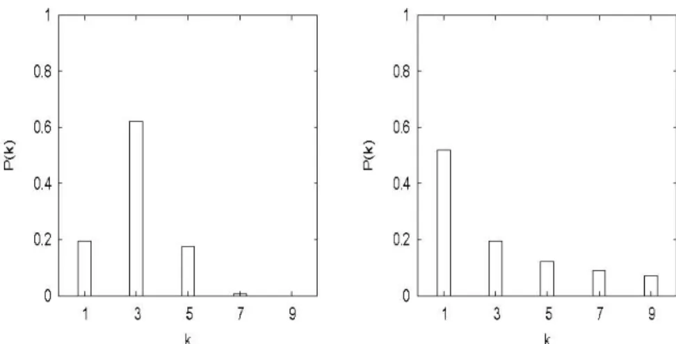
Figure 1. Binomial distribution for q = 0.2527 (left) and Power-law distribution

for γ = 0.898607 (right) with cut-oﬀ at the maximal group size K = 9, respectively.

The average connectivity is in both cases < K > 3≈ .

Here the quantity K represents the maximal group size. Accordingly

and arbitrarily chosen individual belongs to a group of size k with

probabilityP_k. The average connectivity <K> is:

(11)

,

) (

∑

= >

< K

k k P k K

Figure 1 depicts the histogram of a binomial and a power-law

distri-bution for q = 0.2527 and γ =0.898607, respectively. The cut-oﬀ

connecti-vity is chosen as K = 9 which results in five groups of size k∈{1,3,5,7,9}

and an average connectivity < K >≈3.

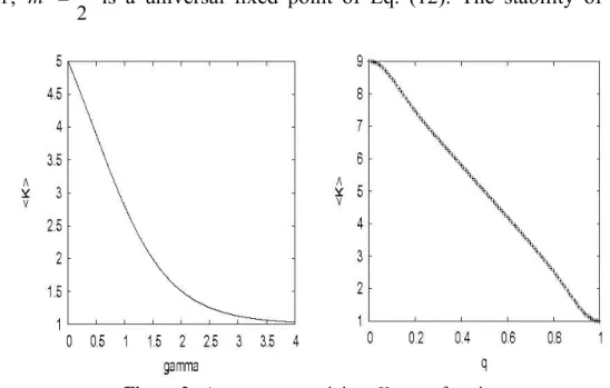
Figure 2 shows the average (eﬀective) connectivity based on a

power-law distribution (left) and a binomial distribution (right) with K = 9.

The eﬀective connectivity < K > is a decreasing function of the control

parameters γ an q. With increasing values of γ and q the connectivity

distributions decrease to their minimum value K = 1. In the following we

assume that a fraction p of the agents follow the local majority rule, while

the fraction (1− p) of the agents obey the local minority rule. Throughout

this study we restrict the fraction of contrarians smaller concentrations

(0 < p < 0.5), since appreciable fractions of contrarians do not reflect the

reality and are irrelevant from a social point of view. The time evolution of

the magnetization m(t) of the

2 1

+

K

component mixture is a linear

(13)

⎜ ⎜ ⎝ ⎛ ⎟ ⎟ ⎠ ⎞ p t m t m j k P p t

m j k j

K

k k

k j

k ⎜_⎝⎛ ⎟_⎠⎞ − +

− =

+ −

+ =

∑ ∑

( )(1 ( ))

) 2 1 ( ) 1 ( ) ( 2 1 (12)

where k runs only over odd values. Since the majority rule as well as the

minority rule is antisymmetric with respect to the interchange of and

, 1 − 1 + 2 1 = ∗

m is a universal fixed point of Eq. (12). The stability of this

Figure 2. Average connectivity <K > as a function

of γ for maximal group size K = 9.

decisive fixed point which was already present in the pure case, gives rise

to a “tie” situation, where 50% of the agents are in favour of the YES and 50% of the agents are in favour of the NO. Note that this subject has often

been discussed in earlier work [2,5]. The critical concentrations are

given by the relation:

m c p . 1 2 1 1 ) 2 1 ( ) ( ) 1 ( 1 ) ( 2 1 2

1_⎟⎟⎜_⎝⎛ ⎟_⎠⎞ =

⎠ ⎞ ⎜ ⎜ ⎝ ⎛ − − = ∂ + ∂ − =

∑

− k K k k m k k k P p t m t m (13)

Solving Eq. (13) for p yields the critical for the bifurcation of

the magnetization and we have:

m c p ⎟ ⎟ ⎟ ⎠ ⎞ ⎜ ⎜ ⎜ ⎝ ⎛ ⎟ ⎟ ⎠ ⎞ ⎜ ⎜ ⎝ ⎛ ⎟ ⎠ ⎞ ⎜ ⎝ ⎛ ⎟ ⎟ ⎠ ⎞ ⎜ ⎜ ⎝ ⎛ − − = − −

∑

− 1 ) ( 1 2 1 1 1 2 1 ) ( 2 1 K k k k m c k k k P K

(14)

The critical concentration for the distance is given by the equation:

) 0

(d∗ →

. 1 ))) ( 1 )( ( ( 1 ) ( ) 1

( ₂1

)

( ₂

1

* ,

0 ⎟⎟_⎠ − =

⎞ ⎜ ⎜ ⎝ ⎛ − = ∂ + ∂ −

∑

− = = k K k

k m t m t

k k P t d t d k m m

d (15)

Since 0 ) ( ) 1 ( = ∂ + ∂ d t d t

d _{reaches its maximum value for} _,

2 1

=

∗

m

inde-pendent of the parameter choice, the Lyapunov stability is guaranteed if:

. 1 1

)

( ₂

1_⎟⎟≤

⎠ ⎞ ⎜ ⎜ ⎝ ⎛ −

∑

− K k k k k k

P (16)

The critical parameter can be calculated by first solving Eq. (15)

for m and inserting this solution into Eq. (12).

d c p

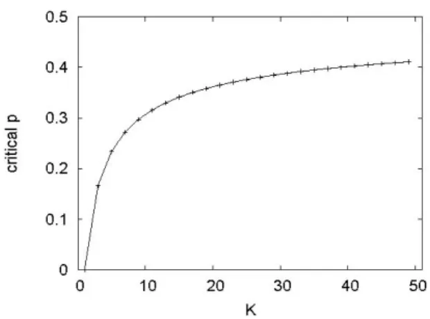
In figure 3 the critical concentration of the contrarians for the “tie” phase

as function of K is represented.

5. Results

Let us first shortly review the basic version of the model [2,3], where

the agents meet in groups of the same size K. For K = 1, where each agent

is only influenced by one single other agent, Eq. (12) becomes:

p t m p t

m( +1)=(1−2 ) ( )+ (17)

with the unique fixed point

2 1

=

∗

m which is always stable in the parameter

range 0 < p < 1. At both extremes p = 0 and p = 1 we have m(t +1) = m(t),

while the time evolution for the distance is always: )

( ) 1

(t d t

d + = (18)

independent of the control parameterp. This implies that the system is

only marginally stable with respect slight changes of the initial condition what the the magnetization and the Hamming distance are concerened. For

general values of K the probability distribution would correspond to the

choice P1 = P3 = ... = PK– 2 = 0, and PK = 1. Due to the symmetry of the

inte-raction rules k P 2 1 = ∗

m is always a natural fixed point of Eq. (12) and

(15)

Figure 3. Critical concentration of the contrarians

for the “tie” phase as a function of K.

Eventually this stationary solution loses its stability below a critical via a bifurcation. In that case, depending on the initial condition, the system can reach one of the two stable fixed points which specify the preference for the YES or the NO. We observe that at low densities of the contrarians, the time evolution of the magnetization Eq. (10) has two attractive fixed points symmetric to

m c p

2 1

which merge at the critical 0.166...

6

1 _≈

=

m c

p for

3

=

K and 0.297...

630

187 _≈

=

m c

p for K =9 via a backward bifurcation [10].

For the system is bistable, while for we have the unique

stable fixed point m

c p

<

p p > p_cm

. 2 1

=

∗

m Correspondingly whenever the ”tie” situation

dominates the system is unstable with respect to small perturbations of the initial configuration. Provided that only one single agent changes its

opinion at an arbitrary time step t, this perturbation can propagate such that

in the long time limit 50% of the agents will have changed their opinion. Around the “tie” we find Gaussian fluctuations with amplitudes

proportional to 1/ N such that the outcome becomes essentially random.

Note however that the magnetization, the acceptance rate of the YES and the NO, is stable, since the individual changes of the votes of the agents cancel out. Figure 3 shows also that the critical concentrations for the

distance are slightly below the corresponding critical values for the

magnetization Figure 4 depicts the long time behaviour of the

magne-tization and the distance for K = 3. It is due to the bifurcation of the

magnetization that eventually a phase transition from chaotic to ordered d

c p

(16)

dynamics occurs when the concentration of the contrarians decreases.

Moreover, the quantity D(t), the distance of the individual follows the

same asymptotics as the Hamming distance between the two replicas d(t)

such that about 50% percent of the of the contrarians change their opinion from one time step to the next. We can conclude that in the whole parameter range of the “tie” the model does not reflect a real life situation,

while below the critical concentration the model is realistic, since

changes in the individual opinion of this magnitude have been reported [13].

Note that for increasing values of K the critical points shift to higher values

of p. Inserting the asymptotic property of the central binomial coefficient:

m c p

K

2 K

K

1

2 1

−

π ≈ ⎟ ⎟ ⎠ ⎞ ⎜ ⎜ ⎝ ⎛ −

− (19)

into Eq. (14) for large values of K we find:

)

(K

p_cm ≈ 1₂− ₈π K. (20)

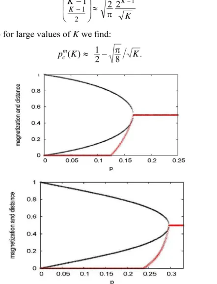
Figure 4. Long time behaviour m* (black) and d* (red) as a function

(17)

Figure 4 depicts the critical concentrations for the phase transition from the “tie” phase to the majority/minority clear cut phase. Small group

sizes K allow only a small fraction of the contrarians to stabilize the

system. Allowing up to about 30% or 25% contrarians we would have to

limit the connectivity parameter to K =10 or K =6, respectively. Note that

these are reasonable upper limits for the concentration of the contrarians [13] as well as for the group sizes. Figure 5 depicts the asymptotic values

of the magnetization and the distance for networks with an average

connectivity <K > =3 (top) and <K > =5 (below), respectively. The right

curves show the pure networks with K =3 and K = 5, where each agent has

exactly K = 3 and K = 5 neighbours. The left curves show the networks based

on a powerlaw distribution, while the middle curves show the networks based on a binomial distribution. Obviously increasing fluctuations around the mean value shift the critical points to smaller values of

m c

m p_cd

pwhich

corres-ponds to effectively lower connectivities. Thorough analysis reveals that

Figure 5. Long time behaviour m* and d* as a function of p for <K >=3 (top) with

(18)

the larger the standard deviation from the mean, the stronger is the shift to the left. One important feature of the networks based on our connectivity

distributions is that with decreasing values of γ and q which reduce the

effective connectivity

k

P

,

>

< K the “tie-region” increases which is consistent

with original pure model [2,5]. On the other hand, with increasing average

connectivity K the chaotic region shrinks such that the region of stability is

expanded. In the limit of γ→∞ as well as the effective connectivity

is

1

→

q 1

= >

< K which leads to the overall stability of the tie-region such that

the time evolution ends up with a tie, independent of the initial condition.

Figure 6 depicts the phase-time portraits in the frozen regime for p = 0.95

with (left), and in the supercritical regime for p = 0.86 with

(right). In the frozen regime we essentially find fixed point behaviour after a short transient. In the supercritical regime we find cycling behaviour of moderate length and observe that a substantial fraction of the agents do not change their state at all. These agents establish a kind of frozen core in the system which is necessary for the existence of the stabil phase. They might be classified as the “inconvincibles” which never change their opinion, independent of the opinion of others. In the chaotic regime we observe that the agents change their opinion more or less randomly. Deep in the disordered phase for

0

=

∗

d d∗ =0.1

2 1

=

∗

d , 50% of the agents change their opinion from

one time step to the next which makes the dynamics quasi-random and unstable. This feature is hardly desirable in a realistic model and might give rise to further discussions and possible improvements of the model.

Figure 6. Space-time diagram for the YES and NO states of the agents for the first hundred time steps for the ordered phase (left) with d∗= 0 and thedisordered

(19)

6. Conclusions

We have shown that the stability of our binary network model governed by a subtle balance of opportunists and contrarians depends crucially on the choice of the degree of the connectivity and on the choice of the of the connectivity structure. The “tie” phenomenon which was already present in the simplest Galam model reminiscent of the hung elec-tions in the US (2000) and Germany (2002), still persists in any genera-lization as long as the symmetry of the interaction rules are preserved. However due to the instability of the system in the relevant parameter range the model does not give a satisfactory answer to the occurrence of the 50%:50% outcome of elections which have been quite popular in the last decade. Galam had suggested that those were not chance driven, but possibly arised due to the coexistence and interplay of opportunists and contrarians [2].

Acknowledgments

The author thanks S. Galam, L. Geyrhofer and F. V. Kusmartsev for various valuable discussions. This work was supported by the Grant FCT PCT/EGE/60193/2004: Modelling Economic Networks, Instituto Superior de Economia e Gestao, Lisboa and by the COST action MP0801 “Physics of Competition and Conflict”, associated with a short term visit of S. Galam at the École Polytechnique, Paris.

REFERENCES

[1] A. L. Barabási and R. Albert, Science 286, 509 (1999).

[2] S. Galam, Physica A 333, 453(2004).

[3] S. Galam, Quality and Quantity, 41, 579-589 (2007).

[4] S. Galam, Europhys. Lett. 70, 705 (2005).

[5] K. E. Kürten, Int. J. Mod. Phys. B 22, 25/26,4674-4683 (2008).

[6] M. Mobilia and S. Redner, Phys. Rev. E 68, 046106 (2003).

[7] K. E. Kürten, Phys. Lett. A 129, 157 (1988).

[8] S. A. Kauffman, Origins of Order: Self-Organization and Selection in Evolution

(Oxford University Press, Oxford) (1993).

[9] D. Stauffer, Extreme Events in Nature and Society, The Frontiers Collection,

Part II, 233-257 (2006).

[10] K. E. Kürten, J. Phys. A: Math. Gen. 21, L615 (1988).

[11] K. E. Kürten and J. W. Clark, Phys. Rev. E, 77, 046116 (2008).

[12] B. Derrida, J. Phys. A, 20, L721(1987).

[13] P. Sciarini and H. Krisi, Int. Journal of Public Opinion Research, 15, 4, 431-453

(20)

AN ECONOPHYSICS MODEL FOR THE

STOCK-MARKETS’ ANALYSIS AND DIAGNOSIS

Ion SPÂNULESCU*, Ion POPESCU**,

Victor STOICA*, Anca GHEORGHIU* and Victor VELTER***

Abstract. In this paper we present an econophysic model for the description

of shares transactions in a capital market. For introducing the fundamentals of this model we used an analogy between the electrical field produced by a system of charges and the overall of economic and financial information of the shares transactions from the stock-markets. An energetic approach of the rate variation for the shares traded on the financial markets was proposed and studied.

Keywords: share, electrostatic field, stock-market, information field,

poten-tial energy.

1. Introduction

The stock exchange rate of a share or other quoted title is the price at which those titles exchange on stock markets. This rate varies according to the law of supply and demand, and the rate approaches more or less the true value of the share.

The setting of the stock exchange rate is based on all available information about the asset proposed for trading, primarily on the intrinsic value estimated by different methods of evaluation of the company or economic entity which is traded on the stock-market. These evaluation methods are based on certain expectations, therefore contain a certain amount of subjectivity depending on the evaluators’ quality, and the model used for it [4]. Therefore, these methods can only give an estimated

potential rate, also called the intrinsic value, which could possibly help the

stock investors in making buying or selling decisions. The problem of the real value arises when the absence of quotation of the asset to the stock market is higher, i.e. the reference price is not fixed yet; in this case

**_{Hyperion University of Bucharest, 169 Calea C}_ă_l_ă_ra_ş_{ilor, St., Bucharest, 030615.} **_{Spiru Haret University, 13 Ion Ghica, St., Bucharest, Romania.}

***_{Valachia University, 2 Carol I, St., Târgovi}_ş_{te, 130024, Dâmbovi}_ţ_{a County,}

(21)

theoretical estimates may serve as a basis for negotiation when taking into account for trading.

In this article, we propose a theoretical model to estimate rate of the share and its evolution over time depending on supply and demand. This model is based on the similarity between an electrostatic field – lizing the stock-market (or field) and the electrical charges which symbol-lizes all the assemble of the economic information about the transactioned shares.

2. The Stock-Markets’ Electrostatic Model

The market value of a share at a certain time t is an average, steady

value, as determined in the negotiated market transactions. The principle followed is that of ensuring counterpart; according to this principle the purchase orders sent to a higher price and the sell orders submitted at a lower price than the market price have their chances of implementing. The accumulation/aggregation of the purchase orders is made from the highest to the lowest rate; the aggregation of the sales orders is made in reverse; the buying and selling orders to the market are primarily/mainly taken into account and are executed at the market rate which is the balance rate (value) at a certain time, when the number is comparable to the offered one.

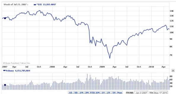
The aggregate evolution of the securities rates on a certain market means the range of values taken by the stock market-rates aggregated in a certain time period subjected to observation on daily basis or in a one day

stock-market session (Fig. 1,c).

Let’s consider the shares Xi of a company C listed on any stock

exchange market.

Suppose that on day z + 1, the stock rate of the shares Xi increases

from 950 monetary units (m.u.) to 1,000 m.u. This growth rate is deter-mined by the establishment of equilibrium between the supply and request/demand at a higher level, thus moving the rate from 950 m.u. on

the day z to 1,000 m.u. on the day z + 1. On the day z + 2, the rate goes up

again to a value of 1,100 m.u. and so on.

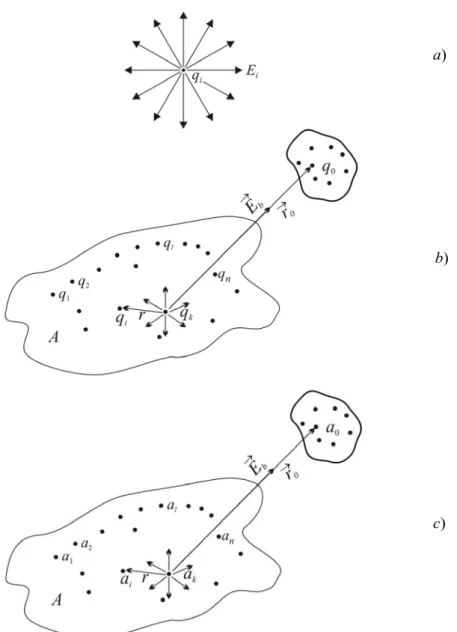
We consider the range of scalar values of equilibrium of the rate of

share Xi as similar to an electrostatic field Ei produced by the charge + qi

symbolizing – in economic terms – all the economic information (price,

(22)

This can be generalized considering that all information about all

shares traded in the stock market A, are sources ai for an information field

Eb symbolizing the whole capital market (Fig. 1,c).

a)

b)

c)

Figure 1. a) Electrostatic field created by electrical change +qi; b) Electrostatic field

created by electrical charges system q1, q2, …qn; c) The stock-market information

field created by a1, a2 …, an information sources.

As the electrostatic field, the stock-market information field is a force

field whose value is proportional to field intensity, E. For example, in

physics the electrical force Fe is [1]:

(23)

where q0 represents an electrical charge. Similarly, the force of the

stock-market quotation of shares, Fb, is given by the law of supply and

request, and can be expressed similar to (1):

Fb = R = aEb (2)

where a represents „the charge” of the point symbolizing the equilibrium

value of a share Xi in the information field.

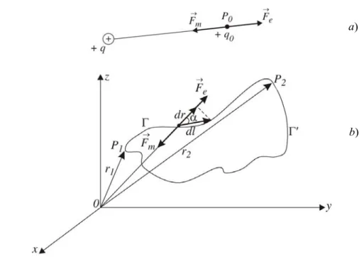
As in physics, to keep a material particle or electrical charge in a

fixed point, the electrical force Fe = qE is compensated by a mechanical

force Fm, in the stock-market field acts the law of supply and demand,

similar to the law of action and reaction in physics (Fig. 2,a).

The electrostatic field created by the charges q1, q2, ...qn, interacts

with the charge q0 located at the distance r0 (Fig. 1,b) through the Coulomb

type electrical force (1) where Fe is given by Coulomb’s Law [1]:

.

41 2

0 1 0 0 r q q F j n j e

∑

πε

= (3)

The total charge Q inside the region A is given by the sum

∑

and 1/ represents the proportionality constant expressed in the

International System of units used in electricity [1]. Comparing the equa-tions (1) and (3), we obtain the equation for the electrical (or electrostatic) field: n j j q 1 , 0 4πε 2 0 0 1 4 1 r q

E n _j j

πε

=

∑

(4)

or: . 2 0 r Q k

E = (5)

In Eq. (5) Q represents the total charge from region A and r0 is the

distance between the region A which creates the field E and the point P0

where is located the charge q0 that the field interacts with (Fig. 1,b). We

notice that the fields’ intensity, thus the influence over q0 charge is smaller

as the distance between the point P0 and the region A is larger (Fig. 1,c).

Similarly, with Eq. (5) we can write equation for the stock-market

information field Eb (Fig. 1,c):

2 0 r Q k E b b

(24)

where r0 represents the so called information, „distance” between the field produced by the figurative points that represent the information „charges”

for the shares contained by a market A (Fig. 1,c) and other share on another

market located at the informational „distance” r0 (Fig. 1,c). It is obvious

that this „distance” will be as longer as big are the difference between the economic and financial information about „the shares”, like the difference between the energy or oil shares and the financial shares for banks or investment funds and so on [2].

Analyzing the region A from figure 1,c, we can see that the

infor-mation distances r between the same type of shares (financial or banking,

for example) are much shorter, so their interaction with the stock-market field is much stronger and the fields’ intensity is much higher:

2 r Q k b

b b

E = (7)

because, as seen in figure 1,b,c, we have r <<r₀. In this latter case,

considering the fields’ interaction Eb with the qi charge from within the

(stock-market) region A, the force of the share given by the equation:

2 r

Q q k

F i

b

k = (8)

is much stronger because of much smaller information „distances” r

com-paring with distance r0.

3. The Energetic Approach

of the Stock-Market Rate

As is known in physics, the fields’ forces can produce mechanical work when acting on a material point or electrical charge on a finite

distance ΔS etc.:

q

.

S F

L = Δ (9)

The electrostatic field E created by the +q charge, will interact with a

test-charge +q0 with a rejection force Fe= q0E seeking to push away the

positive +q0 charge. For the +q0 charge to remain motionless (in

electrostatic terms, standing) is necessary to action with a mechanical force

Fm equal and opposite with the electrical force Fe of the electric field i.e.

(Fig. 2,a):

.

0E q F

(25)

Figure 2. a)Electrical rejection force Fe is compensate by the mechanical force Fm;

b) Calculation of mechanical work of force Fe betwen P1 and P2 points.

The elementary mechanical work dL done by the force Fm when the

charge q0 is moving on the dl displacement (see Fig. 2,b) is given by [1]:

, d ) ( d ) (

dL=Fr_m rr lr=−q₀Er rr lr (11)

where Fr_m(rr), d and lr Er(rr) are vector parameters.

The mechanical work of the force Fm between the points P1 and P2

(Fig. 2,b) is given by:

d ( )d 2 ( )d . (12)

1 2 1 0 2 1 2 ,

1 L F r l q E r l

L r r r r m r r r r r r

∫

= =− =

Taking the axes origin in the center of the source-charge +q and

taking into account the expression (4) will find (following the calculations see [1], p. 39), the equation for the mechanical work:

_⎟⎟ ⎠ ⎞ ⎜⎜ ⎝ ⎛ − πε = πε − =

_∫

1 2 0 0 2 0 0 2 , 1 1 1 4 d 4 2

1 r r

qq r r q q L r r (13) or: ⎟⎟ ⎞ ⎜⎜ ⎛ −

=kq 1 1

L . (14)

⎠

⎝ 2 1

(26)

The equation (14) shows that the mechanical work L1,2 done for the

displacement of the constant charge q0 in the field created by the q charge

from origin does not depend on the path followed between the points P1

and P2, but only on the initial and final position, it means it depends only

on the initial distance r1 and the final distance r2 between origin of axes

and the point P1 and P2 respectively (Fig. 2,b). It is known from mechanics

that such a field having this property (that the mechanical work depends

only on initial and final points) is a conservative field, that means it

possesses potential energy on whose behalf the mechanical work is carried out by the field forces.

Similarly it can be considered that the information stock-market field

Eb is a conservative field where operates the law of supply and request in

the stock-market. The work done by the stock-market field forces is given by an equation similar with Eq. (9):

Lb = R∆P (15)

being determined by the stock-market field forces R, i.e. by the action of

the law of request (Request = R) and offer and by the rate variation ∆P of

the share price.

In equation (15), R represents the stock market force Fb given by the

equation (see Eq. (2)):

b b R aE

F = = (16)

where Eb is the information field of the equilibrium values and other

information regarding the shares, and a represents the „charge” of the point

symbolizing the all information and the shares’ value Xi. The size of R

(Request) represents the reliability degree or appreciation of the considered

share that also determines the level of request R of the share.

Finally, under the action of the field Eb, of the force R, by raising the

request and the offer, and hence the share rate (value), a stock-market „work” is performed given by the equation (see Eq. (9)):

P aE P R

Lb = Δ = bΔ (17)

where ∆P represents the share’s rate variation.

For the conservative fields, like the electrostatic field, the mechanical

work performed at the movement of the charge q0 from the point P1 to the

point P2 (Fig. 2,b) is given by the difference between the potential energies

of the charge q0 in the two points, and that is [1]:

) ( )

( ₂ ₁

2 ,

1 W r W r

(27)

where W(r2) and W(r1) are the potential energies of the „test” charge in the

points P1 and P2 (Fig. 2,b). Similarly, in the stock-market a virtual point

symbolizing all the information about the share Xi from a forces potential

field Eb, like the capital market, possesses the stock-market potential

energy reflected in its price or stock-market rate increase opportunities on

whose behalf the stock-market “mechanical” work is effectuated (Fig. 3): ).

( )

( ₂ ₁

) 2 , 1

( W v W v

L_b = − (19)

If there is a variation of the share rate, from v1 = 950 m.u. to the higher

equilibrium value, for example v2 = 1000 m.u., in this case the equation (19)

for the stock-market work is:

). 950 ( ) 1000 (

) 2 , 1

( W W

L_b = −

Figure 3.

As in mechanics or electrostatics, if the stock-market rate is decree-sing, there is a transformation of the potential energy in kinetic energy, and vice versa for the increasing of the rate. The maximum kinetic energy is achieved in the crush moment until reaching the minimum resistance, than the process can be resumed depending on market development of the value

of the share Xi (Fig. 4).

As it can be seen in figure 4, the successive variations of the transfor-mation of the potential energy into stock-market kinetic energy can take place several times in a one day stock-market session or in other time period represented by the graphics of the evolution of share values. The

minimum value of the potential energy Wpb is when the shares’ rate value

is minimum, thus the share Xi has in that moment a low “potential”. In

(28)

to the variation (raising) speed of the rate and to the transaction time, is

high, the shares’ value can change rapidly, i.e. to increase (Fig. 4) or to begin to decrease again until it reaches a new resistance threshold of the rate.

Figure 4. Weekly evolution of DJI.

4. Conclusions

By similarity with the electrostatic field notion, we can introduce an information field concept for modeling the stock-market shares transactions.

The stock-market information field sources are the points symbo-lizing the totality of economic and financial information about the shares listed at that time.

Similarly with the electrical force notion given by the equation

Fe= qE, where E is an electric field, we propose the introduction of the

notion of stock-market force equal with the request R or with the supply,

and being proportional with the stock-market fields’ intensity with an

information nature, i.e. R = aEb.

The “mechanical” work executed by the forces of the stock-market

field Lb is given by the product between the R force, determined by the law

of supply and request and by the price variation ∆P (the share’s rate

(29)

REFERENCES

[1] Ion Spânulescu, Electricity and Magnetism (in Romanian), Victor Publishing House, Bucharest (2001).

[2] Anca Gheorghiu, Diagnostic-Analysis and Enterprise Valuation (in Romanian), Victor Publishing House, Bucharest (2010).

[3] Anca Gheorghiu and Ion Spânulescu, Macrostate parameter – a new econophysics

and technical index for the stock-market transactions analysis, Proceedings of

ENEC-2009, International Conference, Victor Publishing House, Bucharest, Romania, 2009, pp. 71-87.

(30)

ON APPLICATION OF PHYSICAL MODELS

IN BANKING RISK ESTIMATION:

VALUING THE DEMAND DEPOSITS

Larysa KRASNIKOVA and Ganna BIELENKA*

Abstract. The paper presents a review of existing approaches to valuation of

demand deposits. Special attention is paid to the approach for demand deposits valuation, which is based on relaxation phenomenon. Such phenomenon may be observed in magnetic, ferromagnetic and ferroelectric materials, as well as in the elastic, electric, and magnetic behavior of materials, and is defined as a delay or lag in the response of a linear system, measured relative to the expected linear steady state (equilibrium) values. The bank rate-setting mechanism for demand deposits is found to resemble closely the anelastic relaxations.

The proposed framework may be applied in the course of risk assessment and management in commercial banks, as well as for banking regulatory policy development by supervisory authorities.

Keywords: banking risks, demand deposits, core deposits, relaxation,

anelastic model.

Glossary: Core deposits – the part of customers’ demand accounts that are

expected to remain with a savings institution for a relatively long period of time and may be counted as a stable source of funds for lending.

Demand deposits – accounts from which deposited funds can be withdrawn

at any time without any notice to the depository institution, in contrast to term deposits, which cannot be accessed for a predetermined period.

1. Introduction

One of the popular methods for liquidity and interest rate risk valuation in a bank is gap analysis, applying the allocation of assets and liabilities into a number of time baskets according to the time remaining till their maturity (or revaluation, in case of interest rate gap calculation), with further determination of the gap in each time basket. The positive gap, or excess of assets over liabilities, shows that in the respective time interval a bank is able to cover its liabilities by the maturing assets. The negative gap

*

(31)

implies the necessity of attracting additional financing or selling a part of assets to ensure liability fulfillment, and indicates the presence of liquidity risk (the possibility of not being able to obtain the needed liquidity on the markets, and the risk of bearing excessive costs due to raising additional funding).

A common problem, which arises during liquidity gap profile crea-tion, is related to the fact that calculation requires data both on outstanding balances of bank’s assets and liabilities, and on their maturity schedule. The balances are known, but not necessarily the maturities. Some of the items have no determined maturity and in practice may generate liquidity flows any time, depending on the customer discretion.

Of mentioned items, demand deposits are a case of major importance. First of all, the size of this item is often significant in comparison to liqui-dity stock. Secondly, low rates established on this product make demand deposits a desirable funding source in terms of decreasing the total cost of funding. However, instead the added “cost” of these deposits to a bank is provision to a client of a free option of withdrawal at any day. Thus, the analysis of demand deposits is a necessary and challenging part of asset-liability management, especially useful in liquidity planning and potential liquidity need forecasting, as well as in interest rate risk management.

In the light of recent evolution of physical model application in economics, which allow embracing the key features of decision-making agents’ behavior, the use of such model for demand deposit valuation would provide new insights into the core deposits phenomenon and enable the construction of underlying theory, not just the single model to use.

2. Literature review

The previous research on the topic proposes several solutions to deal with deposits with non-determined maturity. Still, currently there is no agreement on which approach should be used to determine the duration and value of demand deposits.

(32)

One more approach is to divide demand deposits into stable (core) and unstable (volatile) part, based on historical observations path [1,2]. Still, the history may provide not enough information for predicting future outcomes, as the market conditions are changing.

Another approach is to apply modeling in estimating durations of demand deposits. Often, demand deposit balances outstanding or rates on them are being related to variables such as interest rates or economic growth. So, Sheehan [3] proposes to use either Treasury bill rates or the opportunity cost of funds; O’Brien [4] uses 3-month Treasury bill yield; while OTS [5] previously applied secondary-market certificate of deposit yields, and then switched to LIBOR swap yields. The models applied vary from equilibrium-based approach [6] to contingent claims perspective [4,7] to discounted cash-flow modeling [5]. All mentioned works come to the conclusion that the analysis of demand deposits is important for managing financial institution’s profitability.

The analysis of previous literature on the topic reveals the necessity of further research on the topic, as the existing models show lack of coherence with practical rate-setting mechanisms and behavior of market agents. This could potentially lead to over – or under-estimation of actual duration of demand deposit stocks, and as a result, to inconsistency of banking risk estimates.

3. Application of an elastic relaxation framework

for analysis of demand deposits

In order to develop a model for valuation of stable part of demand deposits, it should be taken into account that the rates for such deposits are usually set by a group of decision-making agents in a bank, who react to exogenous market forces (changes in market rates, actions of competitor banks etc.) and seek to maintain the existing balances, and to maximize profits given the presence of market forces. Poorman [8], following Hawkins and Arnold [9], states that in such case, three main postulates may be formulated about the rate-setting mechanism:

1) for every market rate there is a unique equilibrium rate, and vice versa;

2) equilibrium response is achieved only after the passage of suffi-cient time;

(33)

Previously, the attempts were made to approximate this process by regression models trying to capture the relationship between market rate movements and resulting changes in bank-set rates, or by means of partial adjustment models. However, Hawkins and Arnold [9] find the parallel between the above-mentioned postulates and the assumptions underlying the relaxation processes in condensed-matter physics, including magnetic, dielectric, and anelastic relaxations. This allows creating a consistent framework for demand deposits pricing, in which the primary stressor is market rates movement and the response variable is the deposit rate. As Poorman notes, the list of other stressors may comprise costs of deposit servicing, competitor responses, macroeconomic factors and other variables [8].

Relaxation (or hysteresis) in physics is defined as a delay or lag in the response of a linear system, measured relative to the expected linear steady state (equilibrium) values. This phenomenon occurs in magnetic, ferromagnetic and ferroelectric materials, as well as in the elastic, electric, and magnetic behavior of materials, in which a lag occurs between the application and the removal of a force or field and its subsequent effect. Hawkins and Arnold [9] and Poorman [8], examining the bank rate-setting mechanism in the relaxation framework, find that their dynamics is rather close to anelastic relaxations; thus, the models designed for physical relaxation processes analysis may be applied to study the demand deposits.

According to Hawkins and Arnold [9], the above-mentioned postu-lates for relaxation model could be formalized as follows:

;

~p m

Jr c

r = + (1)

(2)

∑

= − − + + = Δ N i p i n i m i n i p

n ar br

r

0

1]. [

Here, equation (1) reflects the first and the third postulates – namely, the existence of equilibrium relationship between the equilibrium rate on demand deposits (~rp)and the market rate J is the share of deposits that the regulatory reserve requirements allow investing.

). (rm

Equation (2) presents the idea of the second postulate about time lag needed for equilibrium response to be achieved, and is built in the form of partial adjustment model with time-dependent notation: r_np =rp(t_n).

It can be noticed that the three postulates formulated and the equilibrium relationship (1) closely resemble the relationship between stress and tension formulated in Hooke’s law of elasticity:

.

ε =

(34)

Here the demand deposit rate would stand for tensile strain (ε), and the market rate would play the role of stress (σ). So, the constant c may reflect the changes in deposit rate produced by different factors (“stresses”).

Further, the differential relationship describing relaxation dynamics may be applied:

. d d ) ( d d m R m p p r J t r J c r t

r ₊_η ₋ ₌ ₊_η_⋅ _⋅

v (4)

Here η denotes the rate, at which the deposit rate relaxes to the equilibrium level, stands for the fraction of response that occurs imme-diately after stress, and is the coefficient for lagged response (at any future time after the stress). Thus, the change in the deposit rate with respect to time is related to the current deposit and market rates, and to the change in market rate with respect to time.

v

J

R J

Equation (4) can be integrated to get the expression for time-dependent deposit rate. Denoting δJ =[J_R −J_v]:

(5) . ]) e 1 [ ( )

( t m

p r J J c t

r = + _v +δ − −η

Of here, the decomposition of the response into instant part and time-dependent part (proportional to

) (J_v

)

J

δ may be obtained: ].

e (6)

1 [ )

(t J J t

J = _v +δ − −η

Boltzmann superposition principle allows rewriting the response function and the time-dependent deposit rate expression, as given in (5) and (6), for the higher orders of the relaxation differential equation, as follows:

∑

(7)

= η − − δ + N i t J J t J 1 ) 1 ( ) 1 ( ] e 1 [ ) ( _v

∑

(8)

= τ − = − M i i m i p t J r c t r 1 ). ( ) (

Here N denotes the order of differential terms included into the relaxation equation, and at the same time the number of relaxation terms. Equation (8) allows determining the demand deposits rate for known history of market rate movements at the consecutive time periods:

m i r . ,..., , ₂

1 τ τM

(35)

Hawkins and Arnold [9], and Poorman [8] state that application of the proposed model to the rates on separate deposit products, such as money market deposit accounts, allowed tracking the respective product rates rather well. This provided the conclusion that “product rates respond to market rates as if via anelastic relaxations” [9]. Therefore, the use of des-cribed model provides the theoretical description for transmission mecha-nism in rate setting for demand deposits and the corresponding factor relationships, and enables calculation of demand deposits rate (and further, duration, based on the assessed rate).

4. Conclusions

The review of existing studies on non-maturing deposits valuation reveals the existence of several approaches to the problem, but each of them has its own advantages and drawbacks. The majority of existing models do not conform to real-life behavior of decision-making agents and market dynamics, proposing only approximate solutions instead of a consistent framework.

Still, the application of physical models may facilitate the creation of a theory underlying the demand deposit movements. This paper reports on the prospective for use of relaxation phenomenon and the related physical models to analyze the demand deposits valuation, allowing to view demand deposits valuation from another angle and to build a consistent framework for their further study.

The anelastic model described can be used in internal risk-manage-ment practices by commercial banks, as well as by supervisory institutions for the purposes of banking regulatory policy development.

R E F E R E N C E S

[1] J. Bessis, Risk Management in Banking, John Wiley & Sons, New York, 1998. [2] Payant, W. R. (2004), An Alternative View of Non-Maturing Deposit Modeling,

Bank Asset/Liability Management, 20(5), pp. 1-3.

[3] Sheehan, R. G. (2004), Valuing Core Deposits, Working Paper, University of Notre Dame.

[4] O’Brien, J. M. (2000), Estimating the Value and Interest Rate Risk of Interest-Bea-ring Transaction Deposits, Finance and Economics Discussion Series 2000-53, Board of Governors of the Federal Reserve System (U.S.).

(36)

[6] Hutchison D. E. & Pennacchi G. G. (1996), Measuring Rents and Interest Rate Risk in Imperfect Financial Markets: The Case of Retail Deposits, Journal of Financial and Quantitative Analysis, 31(3), pp. 399-417.

[7] Jarrow, R. & van Deventer, D. (1998), The arbitrage-free valuation and hedging of demand deposits and credit card loans, Journal of Banking and Finance, 22(3), pp. 249-272.

[8] Poorman, F. A. (2001), Using Physical Models to Describe and Value Core Deposits, Bank Accounting and Finance, December 2001, pp. 17-25.

(37)

MARKET ULTIMATE PROFITABILITY

1

Alexei KAZAKOV* and Maria PLOTNIKOVA**

Abstract. In this article a problem of market research effectiveness is raised

and a method to evaluate it is proposed. The authors introduce a concept of ultimate profitability of any particular market instrument or index. Syste-matic time shifts in market position changes from an ideal timing are consi-dered as a reason of actual profitability declining from ultimate one and are suggested to serve as a measure of market research effectiveness. The ultimate profitability concept itself turns up to be a fruitful one able to reinforce comparative studies of national markets and market tools, invest-ment styles and volatility studies. Following observations of emerging equity markets ultimate profitability characteristics the phenomena of hyper volatility is revealed and a clue to a rationale of high frequency long-short trading are received.

Keywords: market, investments, research, profitability, volatility.

1. Introduction

Economy of portfolio investments

Portfolio investments theory is much about balancing expected return with risk of a desired level. Given that risk is fixed at certain level each portfolio investor strives to enhance yield of investments. In practice the choice is limited: either to increase the gross results of investment activity or to decrease the operating costs, associated with it. It is possible to try to move simultaneously in both directions, but at some moment an increase in a result and reduction in expenditures may start contradicting each other. In particular, so it occurs, if one economizes on research and/or market data processing.

If an investor plans to maintain some level of expenditures on analytical support, then there is a question: whether it is possible to

*1

Occupations as of year 2005 start when the study was conducted.

**

Allianz ROSNO Aseet Management, Post address: Ramenki st., 7/2/351, Moscow, Russian Federation, 119607, e-mail: [email protected].

**

(38)

introduce any criterion for effectiveness of those expenditures? In case an investor is institutional that may be a question of a sizable economic significance.

2. Ideal timing, or the hypothesis about zero shift

Unlike the majority of other costs, which accompany operations on financial markets, expenditures on research – is a rather poorly defined concept, and these costs are subjected to testing on the effectiveness with difficulty. We attempt to estimate the contribution of analytical support to the determination of the optimum moment of changing the market position. To the market participants this process is well known as a choice of right time to enter the market or, in short, the timing. Much of real life investment analytical cases can be transformed / reduced into the form of timing problem.

Let’s accept for an axiom, that the best moments for changing market position are those ones when prices achieve their local extremes – local maximum or minimum values. Let’s imagine that someone can syste-matically determine these price extremes with ideal preciseness. And let’s call this assumption “the hypothesis about zero shift”. In practice things are not so bright: with poor analytical advice an investor risks to take market position far from right moment and/or even not in right direction (which can also be considered as a significant error in a choice of ‘right time’). It is almost self-evident that any actual timing process includes non-zero shifts. A well informed practitioner will tend to make relatively small shifts, while his less prepared competitor will make systematically larger shifts. We’ll consider the average (‘systematic’) proximity of real timing to the ideal one as a criterion of analytical support quality.

3. Market ultimate profitability

3.1. Working Hypothesis

(39)

maximally possible – annual profitability of active investment operations with that market tool, and then it is fixed how this theoretical profitability changes with an increase in a systematic shift of ‘actual’ moments of market position turn (from Long to Short and vice versa) from ‘ideal’ local price extremes. We assume that trading can be done in both directions (up and down) symmetrically easy (i.e. terms for both Buy and Sell Short orders execution are equal).

There is, perhaps, only one problem with this approach: it is possible to reveal multiple extremes of different scale on the price graph. Therefore before taking up the measurement of ultimate profitability, it is necessary to agree about the extent of detailing, needed for studying the price behavior. From mathematical point of view this problem resembles the coastline paradox2, popularized by Benoit Mandelbrot [1]. Thus, we address self-similarity in price behavior by fixing the scale of price move-ments from one extreme to another. Also for the purposes of this study it is more convenient to use percentage measurement of price increments (whereas in fractal studies logarithms are used more often).

After all these assumptions and stipulations have been done we can give clearer definition of what market ultimate profitability is. Average annual ultimate profitability calculated for a number of years shows how much a capital invested in a particular market tool would cumulatively grow in one year (in %) on average, with an assumption that an investor occupies alternately long and short market positions, changing them accurately at the price extremes, which are distant to each other not less than the predetermined value N (in % of entry price). Value N in fact serves similar to a linear measure when determining the distance (in %) overcame by a particular market tool price (remember ‘coastline paradox’). While measuring price movements (from one extreme to another) we ‘don’t notice’ movements less than N. A particular measured movement can be, however, much bigger that N (depending on market dynamics). Ultimate profitability should grow with decreasing N as ‘market distance’ traveled by price increases. In figure 1 the dependence of average annual

2

(40)

ultimate profitability on value N is presented, calculated for Russian equity RUIX index (December 1996-July 2004). Similar experimental curves can be obtained for any tradable asset or market index.

y = 125190x-1.5072

R2_{= 0.9939}

100 1 000 10 000 100 000

0.5% 2.5% 4.5% 6.5% 8.5% 10.5% 12.5% 14.5% 16.5% 18.5%

Variable N - minimal distance betw een price rev ersal points (% of price) Av erage annual ultimate profitability

(%, per annum)

% %

Figure 1. Dependence of average annual ultimate profitability (%) on variable N (%). RUIX index.

Source: RTS.

(41)

3.2. Choice of Scale

Before fixing the scale of market consideration let’s examine the dependence of an average annual ultimate profitability and number of market position reversals (transactions) on parameter N, % based on the Russian equity index RTS (Fig. 2).

0 5 10 15 20 25 30

5 10 15 20 25 30

0 1 000 2 000 3 000 4 000 5 000

RTSI 15 - av erage number of rev ersals per annum (1995-2004) RTSI 15 - av erage number of rev ersals per annum (1999-2004) RTSI - av erage ultimate profitability (1995-2004)

RTSI - av erage ultimate profitability (1999-2004)

%

Average annual number of reversals (trades)

Ultimate profitability,%

N,%

Variable N - minimal distance betw een price rev ersal points (% of price)

Figure 2. Dependence of the average annual number of market position reversals and ultimate profitability on the variable N (%). RTS index.

Source:RTS.

Journal archive

HYPERION

INTERNATIONAL

JOURNAL

CONTENTS

DYNAMICAL STABILITY

OF SCALE-FREE OPINION NETWORKS:

OPPORTUNISTS VERSUS CONTRARIANS

1. Introduction

2. Majority and Minority rules of behaviour

∑

∑

∑

∑

3. Mean field approximation

∑

∑

4. Probability distributions of odd group sizes

∑

∑ ∑

∑

∑

∑

∑

5. Results

6. Conclusions

Acknowledgments

AN ECONOPHYSICS MODEL FOR THE

STOCK-MARKETS’ ANALYSIS AND DIAGNOSIS

1. Introduction

2. The Stock-Markets’ Electrostatic Model

∑

∑

∑

3. The Energetic Approach

of the Stock-Market Rate

∫

∫

∫

∫

4. Conclusions

ON APPLICATION OF PHYSICAL MODELS

IN BANKING RISK ESTIMATION:

VALUING THE DEMAND DEPOSITS

1. Introduction

2. Literature review

3. Application of an elastic relaxation framework

for analysis of demand deposits

∑

∑

∑

4. Conclusions

MARKET ULTIMATE PROFITABILITY

1. Introduction

2. Ideal timing, or the hypothesis about zero shift

3. Market ultimate profitability

3.1. Working Hypothesis

3.2. Choice of Scale

_∫