PATTERN ANALYSIS IN DIMENTIONALITY REDUCTION
Anushiya M 1,Ismail Khan V 2,Nandini S 3,Saravana Kumar S4 1, 2, 3Student, 4Assistant Professor,
Computer Science and Engineering, Adithya Institute of Technology, Coimbatore, Tamilnadu, India.
Abstract — Emergence of pattern analysis has brought about a paradigm shift throughout computer science, such as the fields of computer vision, machine learning and multimedia analysis. Dimensionality reduction is one of the important fields in Machine learning which can be used to reduce the characteristics under consideration thereby reducing the computation and storage. In this project we use Independent Component Analysis to generate pattern for different characteristics of raw data in symbolic form.
The terms pattern recognition, machine learning, data mining and knowledge discovery in databases (KDD) are hard to separate, as they largely overlap in their scope. Machine learning is the common term for supervised learning methodsand originates from artificial intelligence, whereas KDD and data mining have a larger focus on unsupervised methods and stronger connection to business use. In pattern recognition, there may be a higher interest to formalize, explain and visualize the pattern, while machine learning traditionally focuses on maximizing the recognition rates. Yet, all of these domains have evolved substantially from their roots in artificial intelligence, engineering and statistics, and they have become increasingly similar by integrating
developments and ideas from each other.
Keywords—Dimensionality reduction, Independent Component Analysis, Pattern generation, Principle Component Analysis.
I. INTRODUCTION
The major reason for great deal of attention in the industry in recent years is due to the wide availability of huge amount of data and the imminent need for turning such data into useful information and knowledge. The information and knowledge gained, can be used for the application ranging from business management, Production control, and market analysis, to engineering design and science exploration. The task of finding frequent pattern in large databases is very important and has been studied in large scale in the past few years.
II. DATAANALYSIS
Analysis of data is a process of inspecting, cleaning, transforming, and modelling data with the goal of discovering useful information, suggesting conclusions, and supporting decision-making. It involves in obtaining raw data and converting it into information useful for decision-making by users. Data is collected and analysed to answer questions, test hypotheses or disprove theories. Data analysis has multiple facets and approaches, encompassing diverse techniques under a variety of names, in different business, science, and social science domains. Data mining is a particular data analysis technique that focuses on modelling and knowledge discovery for predictive rather than purely descriptive purposes. Business intelligence covers data analysis that relies heavily on aggregation, focusing on business information. In statistical applications, some people divide data analysis into descriptive statistics, exploratory data analysis, and confirmatory data analysis. Data may be numerical or categorical. Data is collected from a variety of sources. The requirements may be communicated by analysts to custodians of the data, such as information technology personnel within an organization. The data may also be collected from sensors in the environment, such as traffic cameras, satellites, recording devices, etc. It may also be obtained through interviews, downloads from
online sources, or reading documentation. Mathematical formulas or models called algorithms may be applied to the data to identify relationships among the variables, such as correlation or causation. Once the data is analysed, it may be reported in many formats to the users of the analysis to support their requirements.
III. SYMBOLICDATAANALYSIS
IV. DIMENSIONALITY REDUCTION
High dimensional data is often found in different disciplines when doing data analysis. The dimension of the data is the number of variables that are measured on each observation. Dimensionality reduction or dimension reduction is the process of reducing the number of random variables under consideration i.e., it produces a compact low-dimensional encoding of a given high-dimensional data set. Its general objectives are to remove irrelevant and redundant data to reduce the computational cost and avoid data over-fitting, and to improve the quality of data for efficient data-intensive processing tasks such as pattern recognition and data mining. Dimensionality reduction can also be seen as the process of deriving a set of degrees of freedom which can be used to reproduce most of the variability of a data set. For high-dimensional datasets (i.e. with number of dimensions more than 10),dimension reduction is usually performed prior to applying a K-nearest neighbours algorithm(k-NN) in order to avoid the effects of the curse of dimensionality. Data dimensionality reduction involves in producing a compact low-dimensional encoding of a given high-dimensional data set. Data visualization involves in providing an interpretation of a given data set in terms of intrinsic degree of freedom, usually as a by-product of data dimensionality reduction. Many algorithms for dimensionality reduction have been developed to accomplish these tasks.
V. IMAGEPROCESSING
Image processing is the processing of images using mathematical operations by using any form of signal processing for which the input is an image, a series of images, or avideo, such as a photograph or video frames. The output of image processing may be either an image or set of characteristics or parameters related to the image. Most image –processing techniques involves two–dimensional signal and applying standard signal processing techniques to it. Images are also processed as three-dimensional signals where the three-dimensional is being time or the z-axis. Image processing usually refers to digital image processing, but opticaland analog image processingalso are possible. This article is about general techniques that apply to all of them. The acquisition of images (producing the input image in the first place) is referred to as imaging. Closely related to image processing are computer graphics and computer vision. In computer graphics, images are manually made from physical models of objects, environments, and lighting, instead of being acquired (via imaging devices such as cameras) from natural scenes, as in most animated movies. Computer vision, on the other hand, is often considered high-level image processing out of which a machine/computer/software intends to decipher the physical contents of an image or a sequence of images (e.g., videos or 3D full-body magnetic resonance scans).In modern sciences and technologies, images also gain much broader scopes due to the ever growing importance of scientific visualization (of often large-scale complex
scientific/experimental data). Examples include microarraydata in genetic research, or real-time multi-asset portfolio trading in finance.In modern sciences and technologies, images also gain much broader scopes due to the ever growing importance of scientific visualization (of often large-scale complex scientific/experimental data). Examples include microarraydata in genetic research, or real-time multi-asset portfolio trading in finance.
PATTERNRECOGNITION
Pattern recognition is a branch of machine learning that focuses on the recognition of patterns and regularities in data, although it is in some cases considered to be nearly synonymous with machine learning. Pattern recognition systems are in many cases trained from labelled "training" data (supervised learning), but when no labelled data are available other algorithms can be used to discover previously unknown patterns (unsupervised learning). In machine learning, pattern recognition is the assignment of a label to a given input value. Pattern recognition is studied in many fields, including psychology, psychiatry, ethology, cognitive science, traffic flow and computer science. Pattern recognition encompasses two fundamental tasks: description and classification. Given an object to analyse, a pattern recognition system first generates a description of it i.e., the pattern and then classifies the object based on that description i.e., the recognition.
The essential problem of pattern recognition is to identify an object as belonging to a particular group. Assuming that the objects associated with a particular group share common attributes more so than with objects in other groups, the problem of assigning an un-labeled object to a group can be accomplished by determining the attributes of the object (i.e., the pattern) and identifying the group of which those attributes are most representative (i.e., the recognition).
Fig-2:Architecture Diagram
GRAPHICAL REPRESENTATION OF A HISTOGRAM
Fig-3:Example of Histogram
Sequence Representation of a Histogram H = {5, 30, 25, 50, 10}
The individual elements of a histogram is accessed/denoted as H(i) where i is the location or index
H (1) = 5, H (2) = 30, H (3) = 25, H (4) = 50, H (5) = 10 Now, the dimensionality reduction technique can be applied on the obtained symbolic data.
In real life, quite often we come across features of interval/ duration/ spread /span /distribution/ image/ temporal signal/ video (Nagabhushan.P, 1995). Histogram is a distribution type feature used for characterizing certain generic objects. In this section we introduce basic definitions and arithmetic with reference to histograms followed by the concept of principal component histograms.
VIII. DEFINITIONS AND ARITHMETIC A.Histogram
The histogram is a count of number of elements within a range or a rectangular bin. The height of the bins represents the number of values that fall within each range.
Sequence Representation of a Histogram
H = { 10, 20, 40, 50, 50, 30, 20}
The individual elements of a histogram is accessed/denoted as H(i) where i is the location or index
H(1) = 10, H(2) = 20, H(3) = 40, H(4) = 50, H(5) = 50, H(6) = 30, H(7) = 20
Unit Histo
A unit histogram UH is a Histogram with all its elements as one.
A null histogram NH is a Histogram with all its elements as zero.
B. Histogram Arithmetic
Given two histograms H1 and H2 defined over same variable 'i' with N number of bins the basic arithmetic operations are defined as:
Histogram addition N
H1 + H2 =
Ʃ
(H1(i) + H2(i)) i=1Histogram subtraction N
H1- H2 =
Ʃ
| H1(i) – H2(i) |i=1
Histogram Multiplication Scalar
N
k * H1 =
Ʃ
k * H1(i) i=1Vector N
H1* H2 =
Ʃ
H1(i) * H2(i) i=1Histogram Division Scalar
N
H1 / k =
Ʃ
H1(i) /k i=1Vector N
H1 / H2 =
Ʃ
H1(i) / H2(i) i=1C. Histo Matrix
A histo matrix is a matrix where all its values are histograms. For instance in a 2 x 2 histo matrix
H11 H12 H21 H22
H11, H12, H21 and H22 are histograms
An identity histo matrix is a matrix where the diagonal elements are unit histos and the remaining elements are null histos.
D. Basic Histo-Matrix Operations Given two histo matrices HM1 and HM2
HM1 = H111 H112 H211 H212
HM2 = H211 H212 H221 H222
Histo Matrix Addition
HM1+ HM2= H111+H211 H112+H212 H121+H221 H122+H222
Histo Matrix Subtraction
HM1
-
HM2=|H111-H211| |H112-H212| |H121-H221| |H122-H222|Histo Matrix Multiplication Scalar
k * HM1= k *H111 k * H112 k * H121 k * H122
Histo Matrix Division Scalar
HM1 / k= H11/k H12/k H21/k H22/k
Vector
HM1/ HM2= HM1* HM2-1
E. Histogram PCA Problem Statement
There are m samples in n-dimensional space. Each feature fi of sample j is of symbolic distribution type (histogram), i.e fij = H where 1<=j<=m and 1<=i<=n. It is required to transform the given n-d histogram features fij to n-d histogram features Fij where F = T(f). Here T represents a feature transformation function which generates the principal components. Each histogram feature is constituted with B number of bins.
F. Computational Aspect
For describing the computational details of principal component method on histogram data set, let us consider an original space of 2-d data set D.
f1 f2 Let D = S1 H11 H12 S2 H21 H22
where S1 and S2 are the samples and f1 and f2 are the histogram features.
And let the resultant principal component data set scores be given as
F1 F2 PCA Scores = S1 H*11 H*12 S2 H*21 H*22 Where,
S1 and S2 are the samples and F1 and F2 are the principal component histogram features.
The variance and covariance of the 2-d data set are computed. Let matrix A, be the variance – covariance matrix. The covariance function is defined as,
A = VarCov(D) = E[(H11-µ1)(H21-µ1)] E[(H21-µ1)(H12-µ2)] E[(H21-µ1)(H12-µ2)] E[(H12-µ2)(H22-µ2)]
where E is the expectation, µ1 and µ2 are mean histograms of f1 and f2 respectively.
µ1 = (1/2) *[H11 + H21] and µ2 = (1/2) * [H12 + H22]
Let X be a column histo matrix of eigenvectors and µ be its corresponding histo vector of eigen values.
[A] [X] = λ[X] …(2.1)
Equation (2.1) can be rewritten as
[A - λI] [X] = 0 ….(2.2) where I is an identity histo matrix of the size that of A. The solution of equation (2.2) can be obtained as follows:
DET(A - λI) = 0 ….(2.3) Since we are considering a 2-d data set, i.e. A is 2 x 2 matrix, equation 2.3 gives B (number of histogram bins) number of quadratic equations in λ. Let the roots of this quadratic equations be λ1i and λ2i corresponding to ith bin of histogram. Thus we obtain B sets of (λ1, λ2).
Now corresponding to ith bin substituting λ1i in equation 2.2
and solving it gives eigen vectors of the form V1 = ai11 x1(i) + ai12 x2(i) where ai11 , ai12 are coefficients of
the eigen vector of dimension 1 (F1) corresponding to ith bin. Similarly corresponding to ith bin substituting λ2i in equation
2.2 and solving it gives eigen vectors of the form V2 = ai21 x1(i) + ai22 x2(i) where ai21 , ai22 are coefficients of
the eigen vector of dimension 2 (F2) corresponding to ith bin.
Now corresponding to ith bin, if the first coefficient of the eigen vector V1 is multiplied with the feature values of dimension 1, second coefficient with the feature values of dimension 2 and combination of the two gives the feature values in dimension 1 of the rotated co-ordinate system.
H*11 = ai11 H11(i) + ai12 H12(i) H*12 = ai21 H11(i) + ai22 H12(i)
dimension 2 and combination of the two gives the feature values in dimension 2 of the rotated co-ordinate system.
H*21 = ai11 H21(i) + ai12 H22(i) H*22 = a
i
21 H21(i) + a i
22 H22(i)
For n dimensional data the first principal component histograms represent the large percentage of the total scene variance, succeeding components (pc-2, pc-3,…pc-n) contains a decreasing percentage of the scene variance. Furthermore, because successive components are chosen to be orthogonal to all previous ones, the data are uncorrelated. Most times, the first few principal components are good enough for classification, thus resulting in dimensionality reduction. As can be understood the computational procedure of histogram PCA demands correspondence between the bins i.e. the bins should be centered at the same position for all histograms. It can be achieved by first normalizing the values along each feature and then synthesizing the histogram symbolic data set. This helps us in maintaining the histogram spread between 0 and 1 for all histograms. Another constraint due the requirement of bin correspondence is that all histograms have to span equal spread or equal number of bins. In our experimentation set up we have chosen histograms with 10 bins.
Experimentation
In order to demonstrate the working of the above formulations we have considered a few symbolic dataset synthesized from conventional data sets (a) 700x3 data (Generated by expanding the data table introduced in (Nagabhushan.P,1995) and subsequently in (Nagabhushan.P,1998) (b) iris data and (c) from a multi-channel 80X data set.
Experimentation results: 700x3 Data
The 700x3 is a data set with 700 samples and three features. This data is a conventional data with 5 classes where there is a clear overlap among the feature values requiring all three features for data modelling. We could achieve dimensionality reduction of this conventional data through PCA and could visualize the five classes 30 with the first two principal components as against no two original features could classify the data into 5 classes. This dataset consists of 700 samples with first 140 belonging to class I, 141-280 to class II, 281-420 to class III, 421 to 560 belonging to class IV and 561-700 to class V. Now in each class, the sample set is divided into seven sample packets with 20 samples in each packet. Histograms are generated for each feature in the sample packet. Thus for each class we obtain seven symbolic objects with histogram features. This results in 35 symbolic objects with three histogram features.
Fig-4 portrays the 700x3 Histogram dataset with 35 samples and 3 histogram features. Fig-5 conveys the variance of the histograms along each feature. As can be understood from Histogram arithmetic the variance histograms can be generated by computing the variance along the individual bins. Fig-6 depicts the principal component histograms. It can be
observed from the results that the principal component histograms would take negative values as well. The main point to be noted is that there is always no harm in considering the principal component histograms as it is (i.e. with negative values) for further classification provided we opt for conventional distance measures like euclidean or citiblock distances between the histograms. But there may be distance measures which would have been defined considering that Histograms bins would always have positive values because it represents the frequency of items. For dealing with such kind of situations the principal component histograms can be subjected to global normalization by considering the maximum and minimum bin values of the entire set of principal histograms. Having obtained the principal component histograms we also compute the variance histograms of the principal component histograms and is shown in fig-7. It can be observed the variance histogram of the first principal component histogram and that of second are high. The third principal component histogram has very low variance values along its bins.
This indicates that the first two principal component histograms are good enough to classify the symbolic sample set. It results in 5 classes with seven samples in each as shown. The Tendogram depicted is obtained through complete linkage clustering.
Fig-4: Experimental aspects
Experimentation results: IRIS Data
was done 5 times with respect to each class and thus we obtain 15 symbolic objects with 4 histogram feature type.
Fig-5: IRIS Histogram
Fig-6: IRIS Variance Histogram
The sampling was tuned to cover all 50 samples belonging to each class. Even in this case the values were normalized along each feature to generate uniform histogram spreads between 0 and 1. Fig-5: depicts the 15 histogram symbolic data set and Fig-6: shows the corresponding variance histogram. The resultant histograms of the principal component analysis is portrayed in figure 6.9 and the corresponding variance histogram in figure 6.10 shows high variance values in the first variance histogram and meager values in the remaining three histograms. This indicates that the first principal component histograms are good enough to achieve classification among these 15 samples. The complete linkage clustering results are shown in fig-7: with the first five samples belonging to set, second five to versicolor and last five to verginica. The overlap between versicolor and verginica seen conventionally, is not observable here.
Fig-7:IRIS Clustering with PCH1
Experimentation results: 80X Data
A set of spatial data comprising the characters 8, O, X has been considered for experimentation purpose. It is because of the overlapping nature of the data with respect to symmetry and the overlapping characteristics due to curvature similarity between „8‟ and „O‟, and linear similarity (crossing lines) between „8‟ and „X‟. This indicates the high mix up in the samples that have been considered and it has always been a challenge to deal with the „8OX‟dataset right from the time an „8OX‟ dataset was introduced by Anil Jain (2004). The spatial data is of 200 x 200 in size. The samples considered are shown in fig-8: along with the font label.
Fig-7: Sample data set
From these samples four spatial signals were generated by sampling at 200 locations along each of the four directions. The features extracted are illustrated in fig-8.
a b
Fig-8: 200 features (the number of white pixel before the first black pixel) (a) along the horizontal direction from bottom to top were extracted. (b) along the vertical direction from left to right
The plot of the feature points of the „character- 8 font-amer‟ along the four directions is given below in fig.
Fig-9: Spatial signals recorded by sampling along four directions of spatial data of ‘8’
directions D1, D2, D3 and D4. Thus it is a 4-channel data. Histograms are generated for the signals from each of the channel resulting in the spatial characters represented by 4 histogram features. Thus we create a dataset of 18 symbolic objects represented by 4 histogram features.
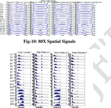
The spatial signals obtained by sampling the characters are shown in fig-10. The corresponding histogram dataset obtained after normalizing the spatial signals are shown in fig-11. The variance histogram of the dataset shows the distribution of variance among all four histogram features in fig-12. After principal component analysis on the histogram data we observe the concentration of variance in the first variance histogram shown in fig-13. Thus the results obtained out of the first principal component histogram is capable enough to classify the „8‟ samples into one group, „0‟ samples into second group and „X‟ samples gets grouped into the third group. The complete linkage clustering results are depicted in fig-14.
Fig-10: 80X Spatial Signals
Figure 6.10 80X Principal Component Histograms
Figure 6.12 80X Variance Histograms of PC Histograms
CONCLUSION
Here, we have predicted the output using symbolic feature extraction and using the technique, Principle Component Analysis in Dimensionality Reduction. It minimizes the data in the data set using dimensionality reduction and gives more storage space. The proposed method hopefully can inspire a new thinking and new way to tackle the pattern analysis problem. This System can be used to generate patterns for various Image Processing applications like stock market, face recognition and analysis of student data.
REFERENCES
[1] H. H. Bock and E. Diday, Analysis of Symbolic Data: Exploratory
Methods for Extracting Statistical Information From Complex Data.
Berlin, Germany: Springer-Verlag, 2000.
[2] Chouakria, P. Cazes, and E. Diday, “Symbolic principal component analysis,” in Analysis of Symbolic Data: Explanatory Methods for Extracting Statistical Information from Complex Data, H.-H. Bock and E. Diday, Eds. Berlin, Germany: Springer-Verlag, pp. 200–212, 2000.
[3] Douzal-Chouakria, L. Billard, and E. Diday, “Principal component analysis for interval-valued observations,” Statist. Anal. Data Mining, vol. 4, no. 2, pp. 229–246, 2011.
[4] F. Gioia and C. Lauro, “Principal component analysis on interval data,” Comput. Statist., vol. 21, no. 2, pp. 343–363, 2006.
[5] C. Lauro and F. Palumbo, “Principal components analysis of interval data: A symbolic data analysis approach,” Comput. Statist., vol. 1, no. 1, pp. 73–87, 2000.
[6] P. Nagabhushan and P. Kumar, “Histogram PCA,” in Advances in Neural
Networks—ISNN 2007 (Lecture Notes in Computer Science), vol. 4492.
Berlin, Germany: Springer, pp. 1012–1021. 70
[7] M. Noirhomme-Fraiture and P. Brito, “Far beyond the classical data models: Symbolic data analysis,” Statist. Anal. Data Mining, vol. 4, no. 2, pp. 157–170, 2011.
[8] O. Rodriguez, E. Diday, and S. Winsberg, “Generalization of the principal components analysis to histogram data,” Proc. PKDD, Lyon,
France, 2000.