SOLVING HIGHER-ORDER INTEGRO DIFFERENTIAL EQUATIONS BY VIM AND MHPM

(1)

ISSN: 1311-1728 (printed version); ISSN: 1314-8060 (on-line version) doi:_{http://dx.doi.org/10.12732/ijam.v33i2.5}

SOLVING HIGHER-ORDER INTEGRO

DIFFERENTIAL EQUATIONS BY VIM AND MHPM Lafta Dawood1, Abdulrahman Sharif2, Ahmed Hamoud3§

1 _{Department of Mathematics} Thi Qar Directorates of Education, IRAQ 2 _{Department of Mathematics, Hodeidah University}

Al-Hudaydah, YEMEN

3 _{Department of Mathematics, Taiz University,} Taiz, YEMEN

Abstract: In this paper, the Variational Iteration Method (VIM) and Mod-ified Homotopy Perturbation Method (MHPM) are applied to solve boundary value problems for higher-order Volterra integro-differential equations. The nu-merical results obtained with minimum amount of computation are compared with the exact solutions to show the efficiency of the methods. The results show that the variational iteration method is of high accuracy, more convenient and efficient for solving Volterra integro-differential equations. Finally, an ex-ample is included to demonstrate the validity and applicability of the proposed techniques.

AMS Subject Classification: 45J05, 65K10, 65H20

Key Words: Volterra integro-differential equation, VIM, MHPM

1. Introduction

The integro-differential equations be an important branch of modern mathe-matics. It arises frequently in many applied areas which include engineering, Received: August 26, 2019 c 2020 Academic Publications

(2)

electrostatics, mechanics, the theory of elasticity, potential, and mathematical physics [4, 8, 5, 6, 9, 10, 20, 28].

In this work, we consider the Volterra integro-differential equation of the second kind as follows:

m

X

j=0

ξj(x)y(j)(x) =f(x) +

Z x

a

K(x, t)G(y(t))dt, (1)

with initial/boundary conditions:

y(r)(a) =br, r = 0,1,2, . . . ,(k−1), (2)

y(r)(b) =cr, r=k,(k+ 1), . . . ,(m−1), (3)

where y(j)(x) is the jth derivative of the unknown function u(x) that will be determined,K(x, t) is the kernel of the equation, a < x≤b, f(x) and ξj(x)

are analytic functions, G(y(t)), is nonlinear analytic function ofy. The br and

cr are constants.

The boundary value problems for higher-order integro-differential equations have been investigated by Morchalo [27] and Agarwal [1] among others. Re-cently, Hamoud (2019) presented an efficient and numerical procedure for solv-ing boundary value problems for higher-order integro-differential equations. A variety of methods, exact, approximate and purely numerical techniques are available to solve nonlinear integro-differential equations. These methods have been of great interest to several authors and used to solve many nonlinear problems. Some of these techniques are Adomian decomposition method [9, 24], modified Adomian decomposition method [17, 18], Variational iteration method [16, 30] and homotopy perturbation method [20] and many methods for solving integro-differential equations [3, 4, 5, 15, 16, 17, 18, 19, 21, 29].

(3)

A variety of powerful methods has been presented, such as the homotopy analysis method [21], homotopy perturbation method [5], operational matrix with Block-Pulse functions method [4], VIM [16] and the Adomian decompo-sition method [9, 24]. Some fundamental works on various aspects of modifi-cations of the Adomian’s decomposition method are given by Araghi [2]. The modified form of Laplace decomposition method has been introduced by Man-afianheris [25]. Babolian et. al, [4], applied the new direct method to solve non-linear Volterra-Fredholm integral and integro-differential equation using opera-tional matrix with block-pulse functions. The Laplace transform method with the Adomian decomposition method to establish exact solutions or approxima-tions of the nonlinear Volterra integro-differential equaapproxima-tions [17]. Recently, the authors have used several methods for the numerical or the analytical solutions of linear and nonlinear Volterra and Fredholm integro-differential equations [11, 12, 13, 14, 22, 23, 24].

In this work, our aim is to solve the boundary value problems for higher-order Volterra integro-differential equations by using VIM and MHPM.

2. Description of the Methods 2.1. Variational Iteration Method (VIM)

This method has been applied to solve a large class of linear and nonlinear problems with approximations converging rapidly to exact solutions.

The main idea of this method is to construct a correction functional form using general Lagrange multipliers. These multipliers should be chosen such that its correction solution is superior to its initial approximation, called trial function. It is the best within the flexibility of trial functions. Accordingly, Lagrange multipliers can be identified by the variational theory [30]. A complete review of VIM is available in [16].

The initial approximation can be freely chosen with possible unknowns, which can be determined by imposing boundary/initial conditions. To illus-trate, we consider the following general differential equation:

(4)

a sequence yn are constructed such that this sequence converges to the exact

solution. The termsynare calculated by a correction functional as follows:

yn+1(t) =yn(t) +

Z t

0

λ(τ)(Lyn(τ) +Ny˜(τ)−f(τ))dτ. (5)

The successive approximation yn(t), n ≥ 0 of the solution y(t) will be readily

obtained upon using the obtained Lagrange multiplier and by using any selective functiony0.

The zeroth approximation y0 may be selected using any function that just satisfies at least the initial and boundary conditions with λ determined, sev-eral approximations yn(t), n ≥ 0 follow immediately. Consequently, the exact

solution may be obtained by using y(t) = lim

n→∞yn(t). (6)

2.2. Modified Homotopy Perturbation Method (MHPM) The homotopy perturbation technique was proposed first by He [5]. In most cases, this method yields very rapid convergence of the series solution, usually few iterations produce very accurate approximate solution [24, 21]. To explain MHPM, we define homotopyH(y, P) by:

H(y, P) = (1−P)F(y) +P L(y), (7) where F(y) is a functional operator with known solution y0 which generally satisfies the boundary conditions. Obviously, from Eq.(7) we have:

H(y,0) =F(y), H(y,1) =L(y), (8) where F(y) is a functional operator with known solution v0, which can be obtained easily. In MHPM, we define

v0=a1+a2x+a3x2+· · ·+amxm−1,

and continuously trace an implicitly defined curve from a starting pointH(y0) to a solution H(κ,1). Applying the perturbation technique Eq.(7), due to the fact that 0≤P ≤1, can be considered as a small parameter. We can assume that the solution of Eq.(1) can be expressed as a series in as follows:

(5)

As P −→ 1, in Eq.(9), in most cases it converges to an approximate solution, i.e.,

κ= lim

P→1y=y0+y1+y2+. . . (10)

3. Main Results

In this section, we shall give an existence and uniqueness results of Eq. (1), with the initial conditions (2) and prove it.

We can rewrite the equation (1) in the form of:

y(x) = L−1 hf(x)

ξk(x)

i +

k−1 X

r=0

(x−a)r

r! br (11)

+γL−1h Z x

a

1 ξk(x)

K(x, t)G(yn(t))dt

i

−L−1h

k−1 X

j=0 ξj(x)

ξk(x)

y(j)(x)i,

so that

L−1 hZ x

a

1 ξk(x)

K(x, t)G(yn(t))dt

i =

Z x

a

(x−t)k

k!ξk(x)

K(x, t)G(yn(t))dt,

and

k−1 X

j=0

L−1hξj(x) ξk(x)

i

y(j)(x) =

k−1 X

j=0 Z x

a

(x−t)k−1_ξ

j(t)

(k−1)!ξk(t)

y(j)(t)dt.

We set

Ψ(x) =L−1hf(x) ξk(x)

i +

k−1 X

r=0

(x−a)r

r! br.

Before starting and proving the main results, we introduce the following hypotheses:

(H1) There exist two constantsα and γj >0, j= 0,1,· · · , k such that, for

any y1, y2 ∈C(J,R)

|G(y1))−G(y2))| ≤α|y1−y2| and

Dj(y₁)−Dj(y2)

(6)

We suppose that the nonlinear terms G(y(x))) and Dj(y) = (_dxdjj)y(x) =

P∞

i=0γij (Dj is a derivative operator),j = 0,1,· · · , k,are Lipschitz

con-tinuous.

(H2) We suppose that for all a < t≤x≤b,and j= 0,1,· · · , k:

γ(x−t)k_K₍_{x, t}₎

k!ξk(x)

≤ θ1,

γ(x−t)k_K₍_{x, t}₎

k!

≤θ2,

(x−t)k−1_ξ

j(t)

(k−1)!ξk(t)

≤θ3,

(x−t)k−1_ξ

j(t)

(k−1)!

≤θ4.

(H3) There exist three functions θ∗₃, θ₄∗, and γ∗ ∈ C(D,_R+), the set of all positive function continuous onD={(x, t)∈R×R:a < t≤x≤b}such that:

θ∗₃ = max|θ3|, θ∗4 = max|θ4|, and γ∗= max|γj|.

(H4) Ψ(x) is bounded function for all x inJ = (a, b]. Theorem 1. Assume that (H1)–(H4) hold. If

0< ψ= (αθ1+kγ∗θ3∗)(b−a)<1, (12) Then there exists a unique solution y(x) to Eqs. (1)−(2).

Proof. _Let_y₁ _and _y₂ _{be two different solutions of Eqs. (1)}₋₍₂₎_,_then

y1−y2

= Z x a

γ(x−t)k_K₍_{x, t}₎

ξk(x)k!

[G(y1)−G(y2))]dt

− k−1 X j=0 Z x a

(x−t)k−1_ξ

j(t)

ξk(t)(k−1)!

[Dj(y1)−Dj(y2))]dt ≤ Z x a

γ(x−t)k_K₍_{x, t}₎

ξk(x)k!

G(y1)−G(y2)) dt − k−1 X j=0 Z x a

(x−t)k−1_ξ

j(t)

ξk(t)(k−1)!

D

j₍_y

1)−Dj(y2)) dt

≤(αθ1+kγ∗θ∗3)(b−a)|y1−y2|,

(7)

Theorem 2. If problem (1)−(2) has a unique solution, then the solution yn(x) obtained from the recursive relation using VIM converges when 0< φ=

(αθ2+kγ∗θ∗4)(b−a)<1.

Proof. _{We have recursive relation:}

yn+1(x)−y(x) = yn(x)−y(x) − L−1h

k

X

j=0

ξj(x)[yn(j)(x)−y(j)(x)]

i

− L−1hγ Z x

a

K(x, t)[G(yn(t))−G(y(t))]dt

i .

If we set, ξk(x) = 1, and Wn+1(x) = yn+1(x)−y(x), Wn(x) = yn(x)−y(x)

sinceWn(a) = 0, then

Wn+1(x) = Wn(x) +

Z x

a

γK(x, t)(x−t)k

k!

h

G(yn(t))−G(y(t))

i dt − k−1 X j=0 Z x a

λ1ξj(t)(x−t)k−1

(k−1)! h

Dj(yn(t))−Dj(y(t))

i dt

−(Wn(x)−Wn(a)). (13)

Therefore,

|Wn+1(x)| ≤ Z x

a

γK(x, t)(x−t)k

k!

|Wn|αdt

+ k−1 X j=0 Z x a

γξj(t)(x−t)k−1

(k−1)!

max|γj||Wn|dt

≤ |Wn|h

Z x

a

αθ5dt+

k−1 X

j=0 Z x

a

θ∗₄|max|γj|i

≤ |Wn|(αθ2+kγ∗θ4∗)(b−a) =|Wn|φ. Hence,

kWn+1k= max

∀x∈J|Wn+1(x)| ≤φmax∀x∈J|Wn(x)|=φkWnk.

Since 0 < φ < 1, then kWnk −→ 0. So, the series converges and the proof is

(8)

4. Numerical Example

In this section, we present the numerical techniques based on VIM and MHPM, to solve Volterra integro-differential equations:

Example 1.

Consider the Volterra integro-differential equation as follow:

y(4)(x)−y(x) =x(1 +ex) + 3ex−

Z x

0

y(t)dt,

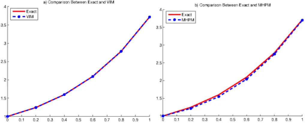
with the boundary conditions: y(0) = 1, y(1) = 1 +e, y′′(0) = 2, y′′(1) = 3e. The exact solution is y(x) = 1 +xex.

x Exact V IM M HP M 0.0 1.00000 1.00000 1.00000 0.2 1.24428 1.24411 1.21187 0.4 1.59673 1.59645 1.54312 0.6 2.09327 2.09296 2.03768 0.8 2.78043 2.78022 2.74460 1.0 3.71828 3.71828 3.70279

Table 1: Numerical Results of Example 1.

5. Conclusion

(9)

Figure 1: Numerical Results of Example 1

References

[1] R.P. Agarwal, Boundary value problems for higher order integro-differential equations, Nonlinear Analysis: Theory, Methods and Appli-cations,7, No 3 (1983), 259-270.

[2] M.A. Araghi, S.S. Behzadi, Solving nonlinear Volterra-Fredholm integro-differential equations using the modified Adomian decomposition method, Comput. Methods in Appl. Math.9 (2009), 321-331.

[3] S.H. Behiry, S.I. Mohamed, Solving high-order nonlinear Volterra-Fredholm integro-differential equations by differential transform method, Natural Science,4, No 8 (2012), 581-587.

[4] E. Babolian, Z. Masouri, S. Hatamzadeh, New direct method to solve non-linear Volterra-Fredholm integral and integro differential equation using operational matrix with Block-Pulse functions, Progress in Electromag-netic Research, B8(2008), 59-76.

[5] M. Ghasemi, M. kajani, E. Babolian, Application of He’s homotopy per-turbation method to nonlinear integro differential equations, Appl. Math. Comput.188 (2007), 538-548.

(10)

[7] A.A. Hamoud, K.P. Ghadle, Existence and uniqueness of the solution for Volterra-Fredholm integro-differential equations,J. of Siberian Federal University. Mathematics &Physics,11, No 6 (2018), 692-701.

[8] A.A. Hamoud, K.P. Ghadle, P.A. Pathade, An existence and convergence results for Caputo fractional Volterra integro-differential equations,Jordan J. of Mathematics and Statistics, 12, No 3 (2019), 307-327.

[9] A.A. Hamoud, K.P. Ghadle, Modified Laplace decomposition method for fractional Volterra-Fredholm integro-differential equations, J. of Mathe-matical Modeling,6, No 1 (2018), 91-104.

[10] A.A. Hamoud, K.P. Ghadle, Homotopy analysis method for the first order fuzzy Volterra-Fredholm integro-differential equations,Indonesian J. Elec. Eng. Comp. Sci.,11, No 3 (2018), 857-867.

[11] A.A. Hamoud, K.P. Ghadle, Some new existence, uniqueness and con-vergence results for fractional Volterra-Fredholm integro-differential equa-tions,J. Appl. Comp. Mech.,5, No 1 (2019), 58-69.

[12] A.A. Hamoud, K.P. Ghadle, Existence and uniqueness of solutions for fractional mixed Volterra-Fredholm integro-differential equations, Indian J. Math.,60, No 3 (2018), 375-395.

[13] A.A. Hamoud, K.P. Ghadle, The approximate solutions of fractional Volterra-Fredholm integro-differential equations by using analytical tech-niques,Probl. Anal. Issues Anal.,7 (25), No 1 (2018), 41-58.

[14] A.A. Hamoud, K.P. Ghadle, S.M. Atshan, The approximate solutions of fractional integro-differential equations by using modified Adomian decom-position method,Khayyam J. of Mathematics,5, No 1 (2019), 21-39. [15] A.A. Hamoud, N.M. Mohammed, K.P. Ghadle, A study of some effective

techniques for solving Volterra-Fredholm integral equations, Dynamics of Continuous, Discrete and Impulsive Systems Ser. A: Mathematical Anal-ysis,26(2019), 389-406.

(11)

[17] A.A. Hamoud, K.H. Hussain, K.P. Ghadle, The reliable modified Laplace Adomian decomposition method to solve fractional Volterra-Fredholm integro-differential equations,Dynamics of Continuous, Discrete and Im-pulsive Systems Series B: Applications and Algorithms,26(2019), 171-184. [18] A.A. Hamoud, K.P. Ghadle, Modified Adomian decomposition method for solving fuzzy Volterra-Fredholm integral equations,J. Indian Math. Soc., 85, No 1-2 (2018), 52-69.

[19] A.A. Hamoud, K.P. Ghadle, M. Bani Issa, Giniswamy, Existence and uniqueness theorems for fractional Volterra-Fredholm integro-differential equations,International Journal of Applied Mathematics,31, No 3 (2018), 333-348; DOI: 10.12732/ijam.v31i3.3.

[20] A.A. Hamoud, A.D. Azeez, K.P. Ghadle, A study of some iterative methods for solving fuzzy Volterra-Fredholm integral equations,Indonesian J. Elec. Eng. Comp. Sci.,11, No 3 (2018), 1228-1235.

[21] A.A. Hamoud, K.P. Ghadle, Usage of the homotopy analysis method for solving fractional Volterra-Fredholm integro-differential equation of the second kind,Tamkang J. of Mathematics,49, No 4 (2018), 301-315. [22] A.A. Hamoud, M. Bani Issa, K.P. Ghadle, M. Abdulghani, Existence

and convergence results for Caputo fractional Volterra integro-differential equations,J. of Mathematics and Applications,41 (2018), 109-122. [23] A.A. Hamoud, M. Bani Issa, K.P. Ghadle, Existence and uniqueness

re-sults for nonlinear Volterra-Fredholm integro-differential equations, Non-linear Functional Analysis and Applications, 23, No 4 (2018), 797-805. [24] K.H. Hussain, A.A. Hamoud, N.M. Mohammed, Some new uniqueness

results for fractional integro-differential equations, Nonlinear Functional Analysis and Applications,24, No 4 (2019), 827-836.

[25] J. Manafianheris, Solving the integro-differential equations using the mod-ified Laplace Adomian decomposition method,J. of Mathematical Exten-sion,6, No 1 (2012), 41-55.

(12)

[27] J. Morchalo, On two point boundary value problem for integro-differential equation of higher order,Fasc. Math.,9 (1975), 77-96.

[28] Y. Salih, S. Mehmet, The approximate solution of higher order linear Volterra-Fredholm integro-differential equations in term of Taylor polyno-mials,Appl. Math. Comput. 112 (2000), 291-308.

[29] S.B. Shadan, The use of iterative method to solve two-dimensional nonlin-ear Volterra-Fredholm integro-differential equations,J. of Communication in Numerical Analysis,2012 (2012), 1-20.