DOI:10.1051/0004-6361/201220959
c
ESO 2013
Astrophysics
&
Chemistry of massive young stellar objects with a disk-like
structure
?
K. Isokoski
1, S. Bottinelli
2,3, and E. F. van Dishoeck
4,51 Raymond and Beverly Sackler Laboratory for Astrophysics, Leiden Observatory, Leiden University, PO Box 9513, 2300 RA Leiden,
The Netherlands
e-mail:[email protected]
2 Université de Toulouse, UPS-OMP, IRAP, 31400 Toulouse, France
3 CNRS, IRAP, 9 Av. Colonel Roche, BP 44346, 31028 Toulouse Cedex 4, France 4 Leiden Observatory, Leiden University, PO Box 9513, 2300 RA Leiden, The Netherlands
5 Max-Planck Institut für Extraterrestrische Physik (MPE), Giessenbachstr. 1, 85748 Garching, Germany
Received 19 December 2012/Accepted 21 March 2013
ABSTRACT
Aims.Our goal is to take an inventory of complex molecules in three well-known high-mass protostars for which disks or toroids have been claimed and to study the similarities and differences with a sample of massive young stellar objects (YSOs) without evidence of such flattened disk-like structures. With a disk-like geometry, UV radiation can escape more readily and potentially affect the ice and gas chemistry on hot-core scales.
Methods. A partial submillimeter line survey, targeting CH3OH, H2CO, C2H5OH, HCOOCH3, CH3OCH3, CH3CN, HNCO,
NH2CHO, C2H5CN, CH2CO, HCOOH, CH3CHO, and CH3CCH, was made toward three massive YSOs with disk-like structures,
IRAS 20126+4104, IRAS 18089-1732, and G31.41+0.31. Rotation temperatures and column densities were determined by the rota-tion diagram method, as well as by independent spectral modeling. The molecular abundances were compared with previous obser-vations of massive YSOs without evidence of any disk structure, targeting the same molecules with the same settings and using the same analysis method.
Results.Consistent with previous studies, different complex organic species have different characteristic rotation temperatures and can be classified either as warm (>100 K) or cold (<100 K). The excitation temperatures and abundance ratios are similar from source to source and no significant difference can be established between the two source types. Acetone, CH3COCH3, is detected for the first
time in G31.41+0.31 and IRAS 18089-1732. Temperatures and abundances derived from the two analysis methods generally agree within factors of a few.
Conclusions.The lack of chemical differentiation between massive YSOs with and without observed disks suggest either that the chemical complexity is already fully established in the ices in the cold prestellar phase or that the material experiences similar physi-cal conditions and UV exposure through outflow cavities during the short embedded lifetime.
Key words.astrochemistry – line: identification – methods: observational – stars: formation – ISM: abundances – ISM: molecules
1. Introduction
Millimeter lines from complex organic molecules are widely as-sociated with high-mass star forming regions and indeed form one of the signposts of the deeply embedded phase of star for-mation (e.g.,Blake et al. 1987;Hatchell et al. 1998;Gibb et al. 2000;Fontani et al. 2007;Requena-Torres et al. 2008;Belloche et al. 2009; Zernickel et al. 2012). Many studies of the chem-istry in such regions have been carried out, either through com-plete spectral surveys of individual sources or by targetting in-dividual molecules in a larger number of sources (see Herbst & van Dishoeck 2009;Caselli & Ceccarelli 2012, for reviews). In spite of all this work, only few systematic studies of the abundances of commonly observed complex molecules have been performed across a sample of massive young stellar ob-jects (YSOs), to search for similarities or differences depend-ing on physical structure and evolutionary state of the object. Intercomparison of published data sets is often complicated by the use of different telescopes with different beams, different fre-quency ranges and different analysis techniques.
?
Appendices are available in electronic form at http://www.aanda.org
Chemical abundances depend on the physical structure of the source such as temperature, density and their evolution with time, as well as the amount of UV radiation impinging on the gas and dust. In contrast with the case of solar-mass stars, the physi-cal structures and mechanisms for forming massive (M >8M)
stars are still poorly understood. Indeed, theoretically, the pow-erful UV radiation pressure from a high-mass protostellar ob-ject (HMPO) should prevent further accretion and so inhibit the formation of more massive stars (Zinnecker & Yorke 2007). However, a number of recent studies have claimed the pres-ence of disk- or toroid-like “equatorial” structures surround-ing a handful of high-mass protostars (Cesaroni et al. 2007). These data support theories in which high-mass star forma-tion proceeds in a similar way as that of low-mass stars via a disk accretion phase in which high accretion rates and non spherically symmetric structures overcome the problem of ra-diation pressure. The best evidence so far is that for a∼5000 AU disk in Keplerian rotation around IRAS 20126+4104, claimed byCesaroni et al.(1999) on the basis of the presence of a veloc-ity gradient in the CH3CN emission perpendicular to the
direc-tion of the outflow, as predicted by the disk-accredirec-tion paradigm. Surprisingly, even in the best case of IRAS 20126+4104, the
A&A 554, A100 (2013)
Outflow
Disk
UV
56
Fig. 1.Illustration of a protostar with a spherical structure (left) and a protostar with a flattened disk-like structure (right) with enhanced UV photons illuminating the walls of the outflow cavity.
detailed chemistry of these (potential) disks has not yet been studied.
Most chemical models invoke grain surface chemistry to cre-ate different generations of complex organic molecules (Tielens & Charnley 1997). Hydrogenation of solid O, C, N and CO dur-ing the cold (Td < 20 K) prestellar phase leads to ample
pro-duction of CH3OH and other hydrogenated species like H2O,
CH4 and NH3 (Tielens & Hagen 1982). Exposure to UV
radi-ation results in photodissociradi-ation of these simple ices, with the fragments becoming mobile as the cloud core heats up during the protostellar phase. First generation complex molecules re-sult from the subsequent recombination of the photofragments, and will eventually evaporate once the grain temperature rises above the ice sublimation temperature of ∼100 K (Garrod & Herbst 2006;Garrod et al. 2008). Good examples are C2H5OH,
HCOOCH3and CH3OCH3 resulting from mild UV processing
of CH3OH ice (Öberg et al. 2009). Finally, a hot core gas phase
chemistry between evaporated molecules can drive further com-plexity in second generation species (e.g., Millar et al. 1991; Charnley et al. 1992,1995).
One of the most obvious consequences of an equatorial rather than spherical structure is that UV radiation can more eas-ily escape the central source and illuminate the surface layers of the surrounding disk or toroid as well as the larger scale envelope (Bruderer et al. 2009,2010) (Fig.1). This can trigger enhanced formation of complex organic molecules in the ices relative to methanol. Another effect of UV radiation is that it drives in-creased photodissociation of gaseous N2and CO. The resulting
atomic N and C would then be available for grain surface chem-istry potentially leading to enhanced abundances of species like HNCO and NH2CHO.
To investigate the effects of disk-like structures on the chemistry, we present here a single-dish survey using the
James Clerk Maxwell Telescope (JCMT) of three HMPOs for
which large equatorial structures (size >2000 AU) have been inferred, namely IRAS 20126+4104, IRAS 18089–1732, and G31.41+0.31. The results are compared with those of a recent survey of a sample of HMPOs byBisschop et al.(2007, here-after BIS07), targeting many of the same molecules and set-tings. The use of the same telescope and analysis method allows a meaningful comparison between the two samples of sources. BIS07 found that the O-rich complex molecules are closely correlated with the grain surface product CH3OH supporting
the above general chemical scenario. N-rich organic molecules do not appear to be correlated with O-rich ones, but overall, the relative abundances of the various species are found to be remarkably constant within one chemical family. One of the main questions is whether this similarity in abundance ratios also holds for sources with disk-like structures. Although our
observations do not spatially resolve these structures, they are sensitive enough and span a large enough energy range to de-termine abundances on scales of∼100 and thereby set the scene for future high-angular resolution observations with interferom-eters like the Atacama Large Millimeter/submillimeter Array (ALMA). Moreover, current interferometers resolve out part of the emission, which is why single-dish observations are still meaningful.
This paper is organized as follows. InSect. 2, the observed sources and frequency settings are introduced and the details of the observations are presented.Section 3 focuses on the data analysis methods. Specifically, two techniques are used to deter-mine excitation temperatures and column densities: the rotation diagram method employed by BIS07 and spectral modeling tools in which the observed spectra are simulated directly.Section 4 presents the results from both analysis methods and discusses their advantages and disadvantages. Finally,Sect. 5 compares our results with those of BIS07 to draw conclusions on simi-larities and differences in chemical abundances between sources with and without large equatorial structures.
2. Observations
2.1. Observed sources
Table1gives the coordinates, luminosity L, distanced, galac-tocentric radiusRGC, velocity of the local standard of restVLSR
and the typical line width for the observed sources. The selected sources are massive YSOs, for which strong evidence exists for a circumstellar disk structure. All sources are expected to harbor a
hot core: a compact, dense (≥107cm−3) and warm (≥100 K) re-gion with complex chemistry triggered by the grain mantle evap-oration (Kurtz et al. 2000). CH3CN emission from≥100 K gas
is present in all sources. Moreover, CH3OH 7K-6K transitions
(338.5 GHz) with main beam temperatures of≥1 K have been observed for these sources. Sources also needed to be visible from the JCMT1.
2.1.1. IRAS 20126+4104
IRAS 20126+4104 (hereafter IRAS 20126) is a luminous (∼104 L
) YSO located relatively nearby at a distance of
1.64 kpc (Moscadelli et al. 2011). It was first identified in the IRAS point source catalog by the IR colors typical of ultracom-pact HII regions and by H2O maser emission characteristic of
high-mass star formation (Comoretto et al. 1990). IRAS 20126 features a∼0.25-pc scale inner jet traced by H2O maser spots in
the SE-NW direction with decreasing velocity gradient (Tofani et al. 1995). Source and masers are embedded inside a dense, parsec-scale molecular clump (Estalella et al. 1993; Cesaroni et al. 1999). The inner jet feeds into a larger scale bipolar out-flow with the two having reversed velocity lobes (Wilking et al. 1990;Cesaroni et al. 1999). The reversal is likely to be due to precession of the inner jet caused by a companion separated by a distance of∼0.500(850 AU) (Hofner et al. 1999;Shepherd et al.
2000;Cesaroni et al. 2005; Sridharan et al. 2005). A rotating, flattened, Keplerian disk structure has been detected perpendic-ular to the inner jet. Observations of CH3CN transitions show a
1 The James Clerk Maxwell Telescope is operated by the Joint
Table 1.Coordinates, luminosity, distance, galactocentric radius, velocity of the local standard of rest,12C/13C isotope ratio and the typical line
width for the observed sources.
Sources α(2000) δ(2000) L d RGC∗ VLSR 12C/13C ∆V
[105L
] [kpc] [kpc] [km s−1] [km s−1]
IRAS 20126+4104 20:14:26.04 +41:13:32.5 0.13a 1.64b 8.3 –3.5 70 6c
IRAS 18089-1732 18:11:51.40 –17:31:28.5 0.32d 2.34e 6.2 33.8 54 5c
G31.41+0.31 18:47:34.33 –01:12:46.5 2.6f 7.9g 4.5 97.0 41 6–10h
Notes.(∗)The galactocentric radii were calculated using distancesdin this table and a IAU recommended distance from the galactic centerR 0=
8.5 kpc. The12C/13C isotope ratios are calculated from Eq. (11).
References.(a)Cesaroni et al.(1997),(b)Moscadelli et al.(2011),(c)Leurini et al.(2007),(d)Sridharan et al.(2002),(e)Xu et al.(2011),(f)Cesaroni
et al.(1994b),(g)Churchwell et al.(1990),(h)Fontani et al.(2007).
Keplerian circumstellar disk (radius∼1000 AU) with a velocity gradient perpendicular to the jet and a hot core with a diameter of∼0.0082 pc and a temperature of∼200 K at a geometric center of the outflow (Cesaroni et al. 1997,1999;Zhang et al. 1998). Direct near-infrared (NIR) observations show a disk structure as a dark line (Sridharan et al. 2005). The disk shows a temperature and density gradient and is going through infall of material with a rate of∼2×10⁻³ M
yr−1 as expected for a protostar of this
mass and luminosity (Cesaroni et al. 2005). Recent modeling of the Spectral Energy Distribution (SED) of IRAS 20126 shows indeed a better fit when a disk is included (Johnston et al. 2011).
2.1.2. IRAS 18089-1732
IRAS 18089-1732 (hereafter IRAS 18089) is a luminous (∼104.5 L, Sridharan et al. 2002) YSO located at a
dis-tance of 2.34 kpc (Xu et al. 2011). It was identified based on CS detections of bright IRAS point sources with colors simi-lar to ultracompact HII regions and the absence of significant free-free emission (Sridharan et al. 2002), and with H2O and
CH3OH maser emission (Beuther et al. 2002). The CO line
pro-file shows a wing structure characteristic of an outflow, although no clear outflow structure could be resolved from the CO maps (Beuther et al. 2002). A collimated outflow in the Northern di-rection is however seen in SiO emission on scales of 500(Beuther et al. 2004). IRAS 18089 has a highly non-circular dust core of ∼3000 AU diameter (∼100), with optically thick CH
3CN at
∼350 K (Beuther et al. 2005). HCOOCH3 was found to be
optically thin, with emission confined to the core, and show-ing a velocity gradient perpendicular to the outflow indicative of a rotating disk (Beuther et al. 2004). Also hot NH3 shows
a velocity gradient perpendicular to the outflow, although no Keplerian rotation was found, possibly due to infall and/or self gravitation (Beuther & Walsh 2008). Several hot-core molecules (HCOOCH3, CH3CN, CH3OCH3, HNCO, NH2CHO, CH3OH,
C2H5OH) were mapped byBeuther et al.(2005) but no column
densities or abundances were reported.
2.1.3. G31.41+0.31
G31.41+0.31 (hereafter G31) is a luminous (2.6 × 10⁵ L
,
Cesaroni et al. 1994b) YSO at a distance of 7.9 kpc (Churchwell et al. 1990). Preliminary evidence for a rotating disk with a perpendicular bipolar outflow was reported by Cesaroni et al. (1994a,b) and Olmi et al.(1996) showing a velocity gradient across the core in the NE-SW direction, similar to previously detected OH masers (Gaume & Mutel 1987). High-angular res-olution CH3CN observations byBeltrán et al.(2005) could not
detect Keplerian rotation typical for less luminous stars, never-theless a toroidal structure undergoing gravitational collapse and fast accretion (∼3×10⁻² M
yr−1) onto the central object was
found. The G31 hot molecular core (HMC) is part of a complex region in which multiple stellar sources are detected (Benjamin et al. 2003); indeed, it is separated from an ultracompact (UC) HII region by only∼500and overlaps with a diffuse halo of free-free emission, possibly associated with the UC HII region itself (Cesaroni et al. 1998). More recent interferometric observations confirm the velocity gradient in the NH3 (4,4) inversion
transi-tion and in CH3CN data (Cesaroni et al. 2010,2011). Line
pro-files look like a rotating toroid with infall motion. Several com-plex hot-core molecules have been observed in G31, including glycolaldehyde CH2OHCHO (Beltrán et al. 2009), but again no
abundance ratios have been presented.
2.2. Observational details
The observations were performed at the JCMT on Mauna Kea, Hawaii, between August 2007 and September 2009. The obser-vations of the 338 GHz region covering CH3OH (7K → 6K)
transitions were taken from JCMT archive. The front ends con-sisted of the facility receivers A3 (230 GHz region) and HARP-B (340 GHz region). The back-end was the digital autocorrelation spectrometer (ACSIS), covering 400 and 250 MHz of instan-taneous bandwidth for A3 and HARP-B, respectively, with a channel width of 50 kHz. The noise level for both receivers was
Trms ∼ 20 mK on aTA∗ scale when binned to 0.5 km s−1. The
integration time was∼1 h and 1.8 h for A3 and HARP-B, re-spectively. The spectra were scaled from the observed antenna temperature,T∗
A, to main-beam temperature,TMB, using main
beam efficienciesηMBof 0.69 and 0.63 at 230 GHz and 345 GHz,
respectively. We adopt aTA∗ calibration error of 20%.
The HPBW (half-power beam width, θB) for the 230 and
345 GHz band observations are 20–2100 and 1400, respectively. Emission from a volume with a source diameterθS ≤ θB
un-dergoes beam dilution described by the beam-filling factor,ηBF:
ηBF=
θ2 S
θ2 S+θ
2 B
· (1)
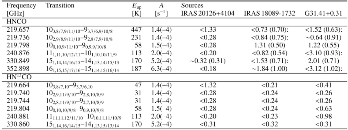
Table 2.Observed frequency settings and molecular lines.
Molecule Freq. Eup µ2S Transition Additional molecules
[GHz] [K] [D2]
CH3CN 239.1195 144.77 811.86 13K–12K CH313CN, HCOOCH3, CH3OCH3
HNCO 219.7983 58.02 28.112 100,10,11–90,9,10 H213CO, C2H5CN
240.8809 112.53 30.431 111,11,12–101,10,11 CH3OCH3, CH3OH, HN13CO
HCOOCH3 222.3453 37.89 42.100 85,4–74,3 CH3OCH3, NH2CHO
225.2568 125.50 33.070 186,12–176,12 H2CO, CH3OCH3,13CH3OH
H2CO 364.2752 158.42 52.165 53,3–43,2 C2H5OH
CH3CN 331.0716 151.11 513.924 18K–17K HCOOCH3, HNCO, CH313CN
HNCO 352.8979 187.25 43.387 161,15,17–151,14,16 C2H5CN, C2H5OH, HCOOCH3
NH2CHO 345.1826 151.59 664.219 170,17–160,16 HCOOCH3, C2H5OH,13CH3OH
HCOOCH3 354.6084 293.39 87.321 332,32–322,31 NH2CHO, C2H5CN
345 GHz, respectively. In order to determine rotation tempera-tures, we covered at least two transitions for a given species with
Eup <100 K andEup>100 K each. BIS07 used the single pixel
receiver B3, the predecessor of HARP-B, together with DAS (Digital Autocorrelation Spectrometer) as the back-end, cover-ing a larger instantaneous bandwidth of 500 MHz. Only the cen-tral receptor of HARP-B array is analyzed here as no significant offsource emission was detected in the complex molecules.
Data reduction and line fitting were done using the CLASS software package2. Line assignments were done by compari-son of observed frequencies corrected for source velocity with the JPL3, CDMS4 and NIST5 catalogs (Pickett et al. 1998; Müller et al. 2005). The line assignment/detection was based on Gaussian fitting with the following criteria: (i) the fitted line po-sition had to be within±1 MHz of the catalog frequency; (ii) the FWHM had to be consistent with those given in Table 1; and (iii) aS/N >3 is required on the peak intensity. Section A.1 in the Appendix describes in more detail the error analysis. In gen-eral, our errors on the integrated intensities are conservative and suggest a lower S/N than that on the peak intensity or obtained using more traditional error estimates.
3. Data analysis
3.1. Rotation diagrams
Rotation temperatures and column densities were obtained through the rotation diagram (RTD) method (Goldsmith & Langer 1999), when 3 or more lines are detected over a suffi -ciently large energy range. Integrated main-beam temperatures, R
TMBdV, can be related to the column density in the upper
en-ergy level by:
Nup
gup
=3k R
TMBdV
8π3νµ2S , (2)
where Nup is the column density in the upper level, gup is the
degeneracy of the upper level,kis Boltzmann’s constant,νis the transition frequency, µis the dipole moment andS is the line
2 CLASS is part of the GILDAS software package developed by
IRAM. 3 http://spec.jpl.nasa.gov/ftp/pub/catalog/catform. html 4 http://www.ph1.uni-koeln.de/vorhersagen 5 http://physics.nist.gov/PhysRefData/Micro/Html/ contents.html
strength. The totalbeam-averaged column densityNT in cm−2
can then be computed from:
Nup
gup =
NT
Q(Trot)
e−Eup/Trot, (3)
whereQ(Trot) is the rotational partition function, andEupis the
upper level energy in K.
Blended transitions of a given species with similar
Eup(∆Eup <30 K) were assigned intensities according to their
Einstein coefficients (A) and upper level degeneracies (gup):
Z
TMBdV(i)=
Z
TMBdV×
Aigi
up
P iAigiup
, (4)
where the summation is over all the contributing transitions. Blended transitions with different Eup, or with contamination
from transitions belonging to other species, were excluded from the RTD fit.
The beam averaged column density, NT, is converted to
thesource-averaged column densityNS using the beam-filling
factorηBF:
NS=
NT
ηBF
· (5)
The standard RTD method assumes that the lines are optically thin. Lines with strong optical depth, determined from the argu-ments in Sect. 4.1 as well as the models discussed in Sect. 3.2, were excluded from the fit. For CH3OH, also low-Eup lines
arising from a cold extended component (see Sect.4.4.1) were excluded.
Differential beam dilution is taken into account by mul-tiplying the line intensities in the 230 GHz range by ηBF
(340 GHz)/ηBF(230 GHz). For warm and cold molecules, beam
dilution is derived assuming source diameters θT=100 K (see
Eq. (10) below) and 1400, respectively (see Eq. (1)). All
emis-sion is thus assumed to be contained within the smallest beam size. Same approach was used in BIS07.
3.2. Spectral modeling
The alternative method for analysing the emission is to model the observed spectra directly. For this purpose, we used the so-called “Weeds” extension of the CLASS software package6, de-veloped to facilitate the analysis of large millimeter and sub-millimeter spectral surveys (Maret et al. 2011). In this model, the excitation of a species is assumed to be in LTE (Local Thermodynamic Equilibrium) at a temperatureTex. The
bright-ness temperature,TB, of a given species as a function of the rest
frequencyνis then given by:
TB(ν)=ηBF
h
Jν(Tex)−Jν
Tbg
i
1−e−τ(ν), (6) whereηBFis the beam filling factor (see Eq. (1)),Jνis the radia-tion field such that:
Jν(T)= hν/k ehν/kT−1
and Tbg is the temperature of the background emission. The
HPBW θB is calculated within the Weeds model as θB =
1.22c/νD, where cis the speed of light and Dis the diameter of the telescope7. The opacityτ(ν) is:
τ(ν)= 8πνc22 NT
Q(Tex)
X
i
Aigiupe−Eupi /kTexehνi0/kTex−1φi (7)
where the summation is over each line i of the considered species.νi
0is the rest frequency of the line andφ
iis the profile
function of the line, given by: φi= 1
∆ν√2πe
−(ν−νi 0)
2/ 2∆ν2
, (8)
where ∆ν is the line width in frequency units at 1/e height. ∆νcan be expressed as a function of the line FWHM in velocity units∆Vby:
∆ν= ν
i
0
c
√
8 ln 2∆V
. (9)
The input parameters in the model are the column density NS
in cm−2, excitation temperatureT
ex in K, the source diameter
θS in arcseconds, offset velocity from the source LSR (Local
Standard of Rest) in km s−1and the line FWHM in km s−1. All
parameters excluding the source diameter are optimized man-ually to obtain the best agreement with the observed spectra. The source diameter for emission from cold species is allowed to vary over a larger area; generally 1400is used. The emission from hot-core molecules targeted in our work is assumed to originate from the central region withTdust ≥100 K. The source diameter
for the warm emission is calculated using a relation derived from dust modeling of a large range of sources (BIS07):
RT=100 K≈2.3×10¹⁴
s L L cm, (10)
whereL/Lis the luminosity of the source relative to the solar
luminosity. Table3gives the calculatedRT=100 Kradii and
diam-eters for the observed sources.
6 CLASS is part of the GILDAS software package developed by
IRAM.
7 For JCMT with 15-m antenna diameter, the equation gives aθ B of
21.900and 14.800for the 230 GHz band and 345 GHz bands, respectively.
Table 3.Source radii and angular diameters forT=100 K.
Sources RT=100K θS,T=100 K
[AU] [00
]
IRAS 20126+4104 1753 2.2
IRAS 18089-1732 2750 2.4
G31.41+0.31 7840 2.0
In the analysis for individual molecules, the initial values for
Tex were based on the Trot from the RTD analysis in case of
optically thin species. For optically thick species the value of
Texfrom the13C-isotope was used. If Texfor the isotopologue
could not be obtained, the initial temperature was guessed. The
Texvalue was then optimized visually based on the relative
in-tensity of the emission lines. The simulated emission was not allowed to exceed the emission of optically thin lines in the spectrum in any of the observed spectral ranges. Coinciding and blended transitions, which together contribute to an optically thick line, are excluded in the analysis.
Due to the visual optimization and the possibility of overlap-ping lines (particularly in the line-rich source G31), the resulting
Texvalues are only a rough estimate (±50–100 K) and do not
dif-fer significantly from those from the RTD method. The column density for each species was constrained by optically thin, un-blended lines, where available.
For the specific case of CH3OH, which requires two
tem-perature components for a proper fit, the analysis was also done with the CASSIS analysis package8. CASSIS has the advantage that it can properly model the emission from overlapping opti-cally thick lines, as well as from nested regions of emission. For CH3OH, warm emission from the compact inner region may be
absorbed by the surrounding colder gas, which can influence the derived hot core abundances.
4. Results
4.1. General results and comparison between sources
The observed sources, IRAS 20126, IRAS 18089 and G31, differ from each other significantly in the observed chemical richness in the JCMT single-dish data. Figure2 presents two frequency ranges with lines from several observed species. For G31, strong lines of all complex organic species are detected, whereas for IRAS 20126 many targeted lines are below the detection limit. Many complex molecules are also found in IRAS 18089 but with weaker lines than for G31. Among the serendipitous discoveries acetone, CH3COCH3, is possibly seen in G31 and IRAS 18089
for the first time (see Sect. 4.5). Integrated line intensities for all detected lines and selected upper limits are given in TablesA.1– A.14. The rotation diagrams for the detected species are shown in Figs. B.1–B.13 whereas the optimized parameters in the Weeds model for each molecule and source are available online in TablesC.1–C.3.
4.2. Optical depth determinations
To assess the importance of optical depths effects, the ratio of lines of different isotopologues are compared. The expected
8 CASSIS has been developed by IRAP-UPS/CNRS (http://
Fig. 2.Spectral ranges 238.83–239.26 GHz and 339.94–340.18 GHz with lines from several targeted species for the three sources.
Table 4.Isotopologue line intensity ratios in the observed sources.
Species IRAS 20126+4104 IRAS 18089-1732 G31.41+0.31
CH3OH/13CH3OH >6 >18 6
CH3CN/CH313CN >65 4.7 4.5
Notes.Lower limits are those for which the13C-isotopologue was not detected.
12C/13C isotope ratio depends on the galactocentric radius,R GC,
according to Eq. (11) (Wilson & Rood 1994).
12C/13C=(7.5±1.9)R
GCkpc+(7.6±12.9). (11)
The isotope ratios derived for our sources using Eq. (11) are given in Table 1. The galactocentric radii were calculated trigonometrically from the galactic coordinates, using the IAU value for the distance to the Galactic centerR0 =8.5 kpc (Kerr
& Lynden-Bell 1986).
Table4lists the observed isotopologue intensity ratios for the most abundant species in our sources. The CH3OH/13CH3OH
ra-tios are derived from a low-energy transition 22,0,+0–31,3,+0with
Eup = 44.6 K. No high Eup transitions were reliably detected
for 13CH3OH in our sources in our standard settings and the
low Eup ratios are therefore taken to apply to cold methanol.
For G31.41+0.31, one additional observation was carried out to cover a transition with Eup > 100 K. A CH3OH/13CH3OH
in-tensity ratio of 4.0 is derived for a transition withEup ≈210 K
(131,12,−0–130,13,+0). This indicates that also warm methanol is
optically thick in this source.
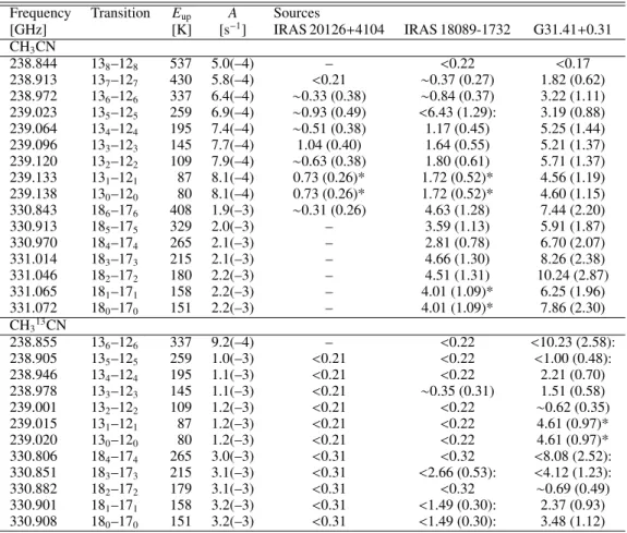
The CH3CN/CH313CN ratios are derived from the 133–123
line intensities for G31 and IRAS 18089 and indicate that CH3CN is optically thick in these two sources, but not in
IRAS 20126. For H2CO and HNCO, isotopologue lines are
de-tected but for different transitions than the main isotopologues. Thus, a model is needed to infer the optical depths. Fits to each of the isotopologues independently at a fixed temperature of 150 K using theRT=100 K source size gives column density
ra-tios that are significantly smaller than the overall isotope rara-tios, suggesting that these species are also optically thick for G31 and IRAS 18089. In practice, we have excluded the optically thick lines (as indicated by the Weeds model) from the RTD fits for all species.
4.3. Temperatures
Table5summarizes the derived temperatures from the RTD fit for the various species. As also found by BIS07, molecules can be classified intocold(<100 K) andwarm(>100 K), and our
cat-egorization is similar to theirs. The Weeds analysis is consistent with this grouping. There is however variation in temperatures within the groups, with warm species having rotation tempera-tures from 70 to 300 K, and cold species from 40 to 100 K. Some variation is seen in rotation temperatures of individual species between different sources; the rotation temperatures are gener-ally higher in G31 than in IRAS 18089, while IRAS 20126 has the lowest of the three.
The Trot value for CH3OH is ∼300 K for G31 and
IRAS 18089 and∼100 K for IRAS 20126. For G31, several lines withEup >400 K are detected, which makes the RTD fit more
robust. For IRAS 18089 and IRAS 20126 the accuracy of the RTD fits suffers from the small range ofEupin the detected
tran-sitions. In addition to optically thick lines, low-Eup lines have
been excluded from the fit. These lines are underestimated by the RTD fit and probably originate from a colder extended region also seen in the13C lines (Fig.3). TheT
rotfrom the RTD
analy-sis therefore represents the warm CH3OH alone. See Sect.4.4.1
for a more detailed discussion on the CH3OH emission.
For CH3CN, theTrotvalues range from∼200 and∼350 K for
the three sources. The CH313CN rotation diagram gives a value
ofTrotof only 53 K, however (Fig.3). This illustrates the large
uncertainties at high temperatures for optically thick species and the possibility of a cold component in addition to the warm one. Contrary to the general trend, the Trot value for H2CO is
somewhat higher (204 K) in IRAS 18089 than in G31 (157 K). The discrepancy could be influenced by the small number of lines used for the analysis. All fitted lines are those belong-ing to the para-H2CO, and the Trot fits are thus not affected
Table 5.Temperatures (K) derived from the RTD analysis and the Weeds or CASSIS (CH3OH) model.
IRAS 20126+4104 IRAS 18089-1732 G31.41+0.31
RTD Model RTD Model RTD Model
warm species
H2CO 123±21 150 204±82 (150) 157±44 (150)
CH3OH 122±17 300, 14±1 291±37 300, 15±2 323±34 200, 14±2
C2H5OH – (100) 85±18 150 120±15 100
HNCO – (200) 92±25 200 111±32 200
NH2CHO – 300 72±28 100 94±50 300
CH3CN 217±352 (200) [346±106] (200) [311±68] (300)
C2H5CN – (80) 84±33 80 105±23 80
HCOOCH3 – (200) 118±20 200 174±11 300
CH3OCH3 – (100) 66±11 100 90±6 100
cold species
CH2CO – (50) 71±11 50 97±101 50
CH3CHO – (50) – (50) – 50
HCOOH – (40) – (40) – 40
CH3CCH 40±10 35 46±12 40 67±14 80
Notes.The species are classifiedwarmandcoldaccording to BIS07. Square bracketed values areTrotvalues for optically thick species and round
bracketed values are Texvalues assumed based on temperatures derived from the other sources in this study. – Means not enough lines were
detected for a rotation diagram. Typical uncertainties in the Weeds excitation temperatures are±50 K.
!
" !
Fig. 3.Rotation diagrams for13CH
3OH (left panel) and CH313CN (right
panel) in G31. Triangles represent blended lines and are not included from the fit.
H213CO (31,2–21,1) was covered, and no information on the
ex-citation temperature can therefore be obtained from the minor isotopologue.
The Trot values of the other complex species, HNCO,
C2H5OH, C2H5CN, NH2CHO and CH3OCH3are around 100 K
and are slightly higher in G31 than in IRAS 18089. TheTrotof
HCOOCH3 stands out in both sources, in G31 being closer to
200 K. No lines belonging to these species were detected in IRAS 20126.
The species classified as cold by BIS07, CH2CO and
CH3CCH, indeed show cold rotation temperatures in all sources.
Not enough lines of CH3CHO or HCOOH, which are also
clas-sified as cold in BIS07, are observed in our sources for making rotation diagrams.
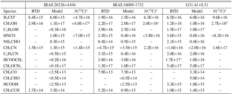
4.4. Column densities
Table 7 presents the column densities derived from the RTD analysis, Weeds or CASSIS model, and from the
13C-isotopologues for the optically thick species. Following
BIS07, the column densities for warm molecules are given as source-averaged values (see Eq. (5)). The emission from cold molecules extends over a larger volume and the values are given
as beam-averaged column densities. Typical uncertainty of the column densities derived from the RTD analysis is∼40%.
4.4.1. CH3OH
An accurate determination of the CH3OH column density is
es-sential for comparing the abundance ratios of complex organic species. For hot-core molecules, it is particularly important to quantify the warm CH3OH emission. The column densities of
CH3OH in BIS07 were determined by the RTD method
exclud-ing the optically thick lines. The same is done in our analy-sis. Our rotation diagrams however also show emission from low-Euptransitions, which are strongly underestimated by the
RTD fit on the warm lines, providing further evidence for the presence of a colder component. We have therefore also ex-cluded these transitions. The fit to the higherEup, optically thin
lines should give the warm CH3OH column density obtained in
a similar way as BIS07.
CH3OH emission was also simulated using a two-component
CASSIS model. A single-component model is not able to simul-taneously reproduce the warm and cold lines without overesti-mating the lines from intermediate energy levels. Indeed, a better agreement is obtained using a two-component model, consisting of a warm compact component and a cold extended component. Table6shows the best model parameters obtained from the fit-ting. The warm components are fixed toθT=100 Kwhile the cold
component is allowed to extend beyond the beam diameter. The warm CH3OH column densities derived from the CASSIS fit are
in agreement with the values derived from the RTD analysis. The best fits plotted onto the CH3OH 7K−6Ktransitions (338.5 GHz)
are shown in Fig.4.
Several 13CH3OH lines are detected in G31. However,
only low-Eup lines are reliably detected since the
high-Eup lines are very weak or blended. Assigning these lines
to the cold component and assuming Trot=20 K (Öberg
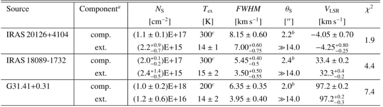
Table 6.CASSIS model parameters for CH3OH in the observed sources.
Source Componenta N
S Tex FWHM θS VLSR χ2
[cm−2] [K] [km s−1] [00
] [km s−1]
IRAS 20126+4104 comp. (1.1±0.1)E+17 300c 8.15±0.60 2.2b −4.05±0.70
1.9 ext. (2.2+−0.90.7)E+15 14±1 7.00+−0.600.75 14.0 −4.25+−0.800.25
IRAS 18089-1732 comp. (2.0+−0.10.2)E+17 300c 5.45+−0.400.5 2.4
b 33.4±0.2
4.4 ext. (2.4+−1.40.5)E+15 15±2 3.50+−0.500.55 14.0 32.3+−0.40.2
G31.41+0.31 comp. (1.0±0.2)E+18 200c 6.35±0.35 2.0b 97.2±0.2
7.4 ext. (1.2±0.6)E+16 14±2 3.95±0.40 14.0 97.2+−0.20.3
Notes.(a)“comp.” for warm, compact component; “ext.” for colder, more extended component.(b)Fixed toθ
s,T=100 K.(c)Fixed.
Fig. 4. CASSIS two-component models for CH3OH emission in the
338 GHz region covering the 7K−6Ktransitions withK=0−6.
13CH
3OH column density is 2.1×1015cm−2, corresponding to a
CH3OH column density of 1.7×1017cm−2for the 1400volume.
This is more than an order of magnitude higher than found in the Weeds model for the cold component, supporting the opti-cally thick interpretation of the cold component. Similarly, for the case of IRAS 18089, the detected13CH
3OH lines may
indi-cate a high optical depth.
As mentioned before, the13CH
3OH line withEup=211 K,
covered in additional observations for G31, reveals optical thick-ness in the warm component as well. The CH3OH column
den-sity derived from this line assuming temperature of 300 K is 2.7× 1018cm−2and the CASSIS fit as well as the RTD analysis
underestimate the warm column density by a factor of∼2.5. In principle, the CASSIS analysis could be made consistent with the 13CH3OH value by letting the warm source size vary as
well. However, since such information is not known for other molecules, as well as for consistency with BIS07, we have cho-sen to keep the warm source size fixed at the 100 K radius.
In summary, it seems plausible that at least in our sources, methanol emission arises from two temperature components, a warm (Tex≈300 K) compact component and a cold (Tex≈20 K)
significantly more extended component. At least for G31, the CH3OH emission is optically thick in both components.
4.4.2. Other molecules
Overall, the column densities of the various species follow the same pattern in all sources, and hence seem to be well correlated
relative to each other. CH3OH is the most abundant complex
molecule in all sources. The other species have in general half to one order of magnitude lower column densities.
The CH3CN emission is optically thick for G31 and
IRAS 18089. Column densities from the RTD analysis are there-fore underestimated. Due to a lack of sufficient optically thin lines, also the Weeds analysis underestimates the column den-sities. Values derived from the13C-isotopologues are thus more
reliable, even though some fraction may arise from a colder com-ponent. Indeed, the column density for CH3CN derived from the
13-isotopologue is an order of magnitude larger than that from the RTD of the main isotopologue alone. The same procedure was used by BIS07.
For H2CO, the best estimates come from the RTD analysis
on the optically thin para-H2CO lines. The derived H2CO
col-umn densities assumingTrotfrom Table5and a statistical
ortho-to-para ratio of 3 are given in Table7. The column densities de-rived from the13C-isotopologue of ortho-H
2CO are still larger
than from RTD analysis using optically thin lines, which indi-cates either larger ortho-to-para ratio in these sources (ratio of∼3 to 5 has been predicted for cold clouds byKahane et al. 1984) or non LTE excitation. BIS07 derived the H2CO column densities
from the13C-isotopologue.
The column density derived for HCOOCH3 from the RTD
diagram is significantly smaller than that derived from the Weeds model. The HCOOCH3 emission is stronger in the 230 GHz
beam (20–2100) than in the 345 GHz beam (1400) probably in-dicating significant extended emission. The RTD analysis was performed on the entire dataset, while only lines in the 230 GHz band was used in the Weeds modeling.
5. Discussion
5.1. Comparison to massive YSOs without a disk structure
Table 7. Column densities for the targeted species from the RTD analysis, Weeds or CASSIS (CH3OH) models and those derived from 13C-isotopologues.
IRAS 20126+4104 IRAS 18089-1732 G31.41+0.31
Species RTD Model N(12C)a RTD Model N(12C)a RTD Model N(12C)a
H2COb 8.4E+15 6.0E+15 <4.7E+16 1.9E+16 1.5E+16 6.3E+16 6.5E+16 6.0E+16 9.6E+16
CH3OH 2.9E+16 1.1E+17 <4.0E+17c 2.2E+17 2.0E+17 2.0E+18c 1.2E+18 1.0E+18 2.7E+18d
C2H5OH – <0.3E+16 – 3.9E+16 2.5E+16 – 1.5E+17 1.0E+17 –
HNCO – 1.0E+15 <7.0E+15 2.5E+15 0.4E+16 <3.8E+16 3.6E+15 0.6E+16 <8.2E+16
NH2CHO – 0.3E+15 – 8.4E+14 0.5E+15 – 2.1E+15 0.4E+16 –
CH3CN 1.5E+15 1.3E+15 <1.4E+15 >4.7E+15 >3.5E+15 2.2E+16 >1.6E+16 >2.0E+16 1.6E+17
C2H5CN – <0.5E+15 – 3.1E+15 0.4E+16 – 2.0E+16 2.0E+16 –
HCOOCH3 – <0.2E+16 – 2.8E+16 3.0E+16 – 1.7E+17∗ 1.0E+18 –
CH3OCH3 – <0.1E+17 – 1.3E+17 1.0E+17 – 5.4E+17 5.0E+17 –
CH2CO – <2.5E+13 – 7.9E+13 7.5E+13 – – 3.3E+14 –
CH3CHO – <0.5E+14 – – <0.5E+14 – – 5.0E+14 –
HCOOH – <2.5E+13 – – <2.5E+13 – 3.2E+15 1.0E+15 –
CH3CCH 2.7E+14 3.5E+14 – 5.2E+14 0.9E+15 – 1.0E+15 1.4E+15 –
Notes.Column densities for the warm molecules are source-averaged, while those for cold molecules are beam-averaged. Column densities where optical depth has a significant effect are labeled as lower limits.(∗)Rotation diagram fit on HCOOCH
3on all lines, while Weeds model on the 230
GHz lines only.(a)N(12C) obtained from theN(13C) adopting a12C/13C ratio equal to 70, 54 and 41 for IRAS 20126, IRAS 18089 and G31.41,
respectively.(b)Column density from13C-isotopologue from ortho-H
213CO, corrected using the statistical ortho to para ratio of 3:1.(c)Calculated
from the line intensity of transition 22,0,+0–31,3,+0at 345.084 GHz withEup=44.6 K, assuming aTrotof 300 K.(d)Calculated from the line intensity
of transition 131,12,−0–130,13,+0at 341.132 GHz withEup=206 K, assuming aTrotof 300 K.
Fig. 5.Source-averaged column densities for the targeted warm species inθT=100 Kvolume. Column densities from the RTD analysis are marked in
black bars. The red and blue bars show column densities from the Weeds or CASSIS (CH3OH) models and from13C-isotopologue, respectively.
Arrows indicate upper limits.
5.1.1. Rotation temperatures
Figure7shows the rotation temperatures of the complex species for the observed sources together with those from BIS07. As in BIS07, we find that the complex molecules can be divided into warm and cold species based on their rotation temperatures. The rotation temperatures obtained for the molecules in our sources agree with the division; CH3OH, H2CO, C2H5OH, HCOOCH3,
CH3OCH3, HNCO, NH2CHO, CH3CN and C2H5CN show
ro-tation temperatures generally≥100 K while CH2CO, CH3CHO,
HCOOH and CH3CCH have rotation temperatures<100 K.
The rotation temperatures of the cold molecules show a very small scatter (±25 K) from source to source, with or without a disk structure, ignoring the one outlier for HCOOH. Of the
warm species, C2H5OH has a consistent rotation temperature of
100–150 K from source to source. The RTD analysis for these species is reliable due to low optical depths and lack of anoma-lous excitation.
The other warm species show more scatter in the de-rived rotation temperatures. This is particularly the case for CH3OH and CH3CN, which have rotation temperatures
rang-ing from 100 to 350 K. No systematic difference is seen be-tween the two source types. Moreover, the HCOOCH3rotation
Fig. 6.Beam-averaged column densities for the targeted cold species. Column densities from the RTD analysis are marked in black bars while the red bars show column densities from the Weeds model. Arrows in-dicate upper limits.
temperatures, but it may also be caused by optical depth ef-fects (H2CO, HNCO, CH3OH and CH3CN) and (anomalous)
ra-diative excitation. The latter has been previously seen for, e.g., NH2CHO and HCOOCH3 (Nummelin et al. 2000) as well as
HNCO (Churchwell et al. 1986). For species with significant ra-diative excitation, e.g., HCOOCH3, the scatter of the data points
in the RTD plots is higher and results in additional uncertainty since the linear fits do not properly capture this scatter.
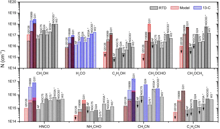
5.1.2. Column densities
Figures 8 and 9 show the column densities for the targeted species in our sources and those from BIS07 for warm and cold molecules, respectively. For the warm species the column densi-ties within the sources vary by 1–2 orders of magnitude. There is also a significant variation between sources. G31 is chemi-cally richest of the sources, with highest column densities of all the targeted species, compared to other sources. IRAS 20126 is among the chemically poorest sources. The pattern of column densities is remarkably similar, however, and the disk sources do not stand out.
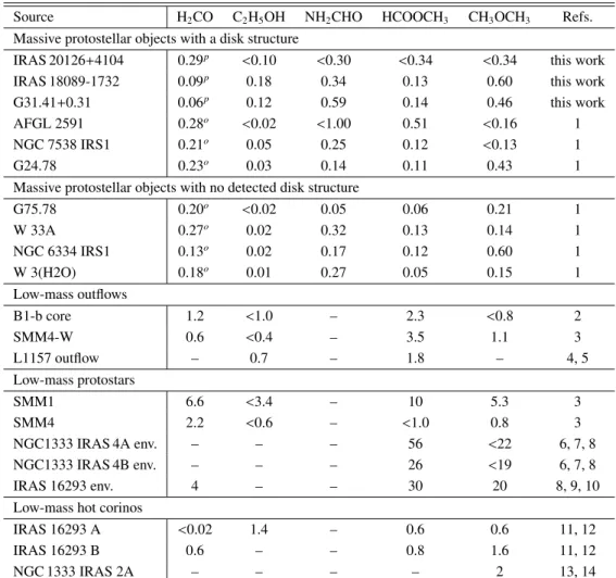
5.1.3. Abundance ratios
Table8gives the abundance ratios for the targeted species with respect to CH3OH for oxygen-bearing species and HNCO for
nitrogen-bearing species. Column densities from the RTD anal-ysis are primarily used. In cases where column densities are not available from the RTD analysis (mainly for IRAS 20126) the values are taken from the Weeds analysis.
The resulting abundance ratios are presented in Fig. 10. Values from the RTD method are shown in black bars and can thus be directly compared to BIS07, whereas those from the Weeds model and 13C-isotopologue are in red and blue bars. In general, the abundance ratios in different sources have larger variations within the source types than between them. For ex-ample, H2CO has both lowest and highest abundance ratio for
two disk candidates, G31 and IRAS 20126, respectively. The H2CO results depend somewhat on the analysis method used.
C2H5OH, HCOOCH3 and CH3OCH3 abundances peak for
G31 and IRAS 18089, and are generally lower for other sources. CH3OCH3also peaks for some diskless sources. The N-bearing
species NH2CHO has a large variation in the abundance ratio
with respect to HNCO. Among our sources, NH2CHO peaks for
G31, the source with largest abundance of O-bearing species, and the least clear disk structure.
Figure11shows the abundance ratios of N-bearing species with respect to CH3OH. Again, a lot of variation is seen within
each source type, with no specific trend found for sources with a disk-like structure.
We stress that the absolute inferred column densities and abundance ratios are uncertain by a factor of a few up to an or-der of magnitude, as already indicated by the different analysis techniques. An independent assessment of the accuracy of the re-sults can be made by comparison with the inferred column den-sities and abundances ofZernickel et al.(2012) for NGC 6334 I (=NGC 6334 IRS), who observed a completely different set of lines of the same molecules withHerschel-HIFI and the SMA in beams ranging from 2–4000. Comparison with the results of BIS07 shows good agreement within a factor of a few for the abundances of several species (CH3OH, CH3OCH3, CH3OCHO,
C2H5OH, C2H5CN) whereas others differ by an order of
mag-nitude (H2CO, CH3CN). The species that show the largest
dis-crepancy are those with highly optically thick lines and without a large set of isotopologue lines. Thus, a combination of dif-ferences in adopted source sizes and optical depth effects can account for the discrepancies. Because our approach is the same for all sources, the relative values from source to source should be more reliable.
5.2. Chemical and physical implications
The main goal of this study is to investigate similarities and differences between sources with and without a disk-like struc-tures. The presence of a flattened accretion disk should allow the UV radiation from the central object to escape more read-ily and then impinge on the gas and dust in the outer walls of a flared disk or outflow cavity (Bruderer et al. 2010). Increased UV radiation could manifest itself as enhancement in the com-plex organic species produced through UV photodissociation from CH3OH in the solid state, such as CH3OCH3, C2H5OH
and CH3OCHO (Öberg et al. 2009). In this scenario, CH3OH is
photodissociated into various radicals such as CH3, CH3O and
CH2OH which can become mobile at higher ice temperatures
(20–40 K) and form the observed complex organic molecules (Garrod & Herbst 2006). Higher temperatures favor diffusion of larger radicals resulting in the formation of larger complex organic molecules compared with small molecules like H2CO.
Another related parameter that plays a role is the CO content of ices, with H2CO, CHO- and COOH-containing species enriched
in cold, CO-rich CH3OH ices in which CO has not evaporated.
IndeedÖberg et al.(2011) show that the increased abundance of HCOOCH3in low-mass YSOs compared with the high-mass
sample of BIS07 may be due to this effect. Although only lim-ited laboratory experiments exist on N-containing molecules, the abundance of N-bearing complex organic molecules could be en-hanced due to photodissociation of N2or NH3.
Our results show that there is no consistent enhancement of complex organic species produced through CH3OH
Fig. 7.Rotation temperatures for selected species in massive YSOs with (open stars) and without (asterisks) observed disk structure.
Fig. 8.Source-averaged column densities for warm molecules. Column densities from the RTD analysis are marked in black bars. Sources without disk structure are marked with an asterisk. The red and blue bars show column densities from the Weeds or CASSIS (CH3OH) models and from 13C-isotopologue, respectively. Upper limits are indicated with arrows.
which UV radiation can escape and affect the chemistry, whether or not they have a large disk-like structure. This scenario can be tested with future high angular resolution data on<100 scale
with ALMA which should then reveal the emission from com-plex molecules coating the walls of the outflow cavities.
An alternative explanation is that enhanced temperature in the YSO environment is not needed for the production of com-plex organic molecules and that they are already formed in the prestellar stage through UV- and cosmic-ray processing of cold ices, using just the internal UV field produced by interaction of cosmic rays with H2(Prasad & Tarafdar 1983) rather than that of
the star. This scenario has gained support over the last few years
with the detection of HCOOCH3 and CH3OCH3 in cold
low-mass cores away from the YSO where the molecules are either released by shocks (Arce et al. 2008;Öberg et al. 2010) or by photodesorption (Bacmann et al. 2012) although the precise for-mation mechanisms are still unclear. Gas-phase processes may also contribute in some cases. Again, high spatial resolution and sensitivity such as ALMA will be key to testing this scenario.
6. Summary and conclusions
Fig. 9.Beam-averaged column densities for cold molecules in sources observed in this study and those from BIS07. Sources without disk structure are marked with an asterisk. Column densities from the RTD analysis are marked in black bars while the red bars show column densities from the Weeds model. Upper limits are indicated with arrows.
Table 8.Abundance ratios of complex species in the observed sources and those in other chemically rich environments.
Source H2CO C2H5OH NH2CHO HCOOCH3 CH3OCH3 Refs.
Massive protostellar objects with a disk structure
IRAS 20126+4104 0.29p <0.10 <0.30 <0.34 <0.34 this work
IRAS 18089-1732 0.09p 0.18 0.34 0.13 0.60 this work
G31.41+0.31 0.06p 0.12 0.59 0.14 0.46 this work
AFGL 2591 0.28o <0.02 <1.00 0.51 <0.16 1
NGC 7538 IRS1 0.21o 0.05 0.25 0.12 <0.13 1
G24.78 0.23o 0.03 0.14 0.11 0.43 1
Massive protostellar objects with no detected disk structure
G75.78 0.20o <0.02 0.05 0.06 0.21 1
W 33A 0.27o 0.02 0.32 0.13 0.14 1
NGC 6334 IRS1 0.13o 0.02 0.17 0.12 0.60 1
W 3(H2O) 0.18o 0.01 0.27 0.05 0.15 1
Low-mass outflows
B1-b core 1.2 <1.0 – 2.3 <0.8 2
SMM4-W 0.6 <0.4 – 3.5 1.1 3
L1157 outflow – 0.7 – 1.8 – 4, 5
Low-mass protostars
SMM1 6.6 <3.4 – 10 5.3 3
SMM4 2.2 <0.6 – <1.0 0.8 3
NGC1333 IRAS 4A env. – – – 56 <22 6, 7, 8
NGC1333 IRAS 4B env. – – – 26 <19 6, 7, 8
IRAS 16293 env. 4 – – 30 20 8, 9, 10
Low-mass hot corinos
IRAS 16293 A <0.02 1.4 – 0.6 0.6 11, 12
IRAS 16293 B 0.6 – – 0.8 1.6 11, 12
NGC 1333 IRAS 2A – – – – 2 13, 14
Notes.The abundances are column densities with respect to CH3OH for oxygen-bearing species and with respect to HNCO for nitrogen-bearing
species. The CH3OH and HNCO column densities are taken from the RTD analysis when available.(p)Para-H2CO.(o)Ortho-H2CO.
Fig. 10.Abundance ratios of complex species with respect to CH3OH for oxygen-bearing species and HNCO for nitrogen-bearing species. The
black bars indicate abundance ratios calculated with the CH3OH and HNCO column density derived from the RTD analysis similar to BIS07.
The red and blue bars indicate abundance ratios where CH3OH and HNCO column densities are derived from CASSIS or Weeds (HNCO) model,
respectively. Upper limits are marked with arrows.
Fig. 11.Abundance ratios of N-bearing species HNCO, CH3CN, C2H5CN and NH2CHO with respect to CH3OH (from RTD analysis). Arrows
indicate upper limits.
YSOs with strong evidence of circumstellar accretion disks, IRAS 20126+4104, IRAS 18089-1732 and G31.41+0.31. This is the first time that molecular abundances are reported for these well-known sources. The analysis is performed using both the rotation diagram method and spectral modeling. The inferred rotation temperatures and molecular abundances are compared to sources without reported disk structures analyzed using the same techniques. The molecules can be divided into two diff er-ent groups based on their rotation temperatures, independer-ent of source type. In particular, the cold (<100 K) species have re-markably constant rotation temperatures from source to source. The warm (>100 K) species exhibit more scatter possibly due to optical depth effects, non-LTE conditions and radiative ex-citation. The column densities peak for the same sources, with G31.41+0.31 being chemically the richest of the studied sources.
Acknowledgements. Astrochemistry in Leiden is supported by the Netherlands Research School for Astronomy (NOVA), by a Spinoza grant from the Netherlands Organisation for Scientific Research (NWO), and by the European Community’s Seventh Framework Programme FP7/2007-2013 under grant agreement 238258 (LASSIE) and 291141 (CHEMPLAN).
References
Arce, H. G., Santiago-García, J., Jørgensen, J. K., Tafalla, M., & Bachiller, R. 2008, ApJ, 681, L21
Bachiller, R., & Perez Gutierrez, M. 1997, ApJ, 487, L93
Bacmann, A., Taquet, V., Faure, A., Kahane, C., & Ceccarelli, C. 2012, A&A, 541, L12
Belloche, A., Garrod, R. T., Müller, H. S. P., et al. 2009, A&A, 499, 215 Beltrán, M. T., Cesaroni, R., Neri, R., et al. 2005, A&A, 435, 901
Beltrán, M. T., Codella, C., Viti, S., Neri, R., & Cesaroni, R. 2009, ApJ, 690, L93
Benjamin, R. A., Churchwell, E., Babler, B. L., et al. 2003, PASP, 115, 953 Beuther, H., & Walsh, A. J. 2008, ApJ, 673, L55
Beuther, H., Schilke, P., Sridharan, T. K., et al. 2002, A&A, 383, 892 Beuther, H., Hunter, T. R., Zhang, Q., et al. 2004, ApJ, 616, L23 Beuther, H., Zhang, Q., Sridharan, T. K., & Chen, Y. 2005, ApJ, 628, 800 Bisschop, S. E., Jørgensen, J. K., van Dishoeck, E. F., & de Wachter, E. B. M.
2007, A&A, 465, 913 (BIS07)
Bisschop, S. E., Jørgensen, J. K., Bourke, T. L., Bottinelli, S., & van Dishoeck, E. F. 2008, A&A, 488, 959
Blake, G. A., Sutton, E. C., Masson, C. R., & Phillips, T. G. 1987, ApJ, 315, 621 Bottinelli, S., Ceccarelli, C., Williams, J. P., & Lefloch, B. 2007, A&A, 463, 601 Bruderer, S., Benz, A. O., Doty, S. D., van Dishoeck, E. F., & Bourke, T. L.
2009, ApJ, 700, 872
Bruderer, S., Benz, A. O., Stäuber, P., & Doty, S. D. 2010, ApJ, 720, 1432 Caselli, P., & Ceccarelli, C. 2012, A&ARv, 20, 56
Cazaux, S., Tielens, A. G. G. M., Ceccarelli, C., et al. 2003, ApJ, 593, L51 Cesaroni, R., Churchwell, E., Hofner, P., Walmsley, C. M., & Kurtz, S. 1994a,
A&A, 288, 903
Cesaroni, R., Olmi, L., Walmsley, C. M., Churchwell, E., & Hofner, P. 1994b, ApJ, 435, L137
Cesaroni, R., Felli, M., Testi, L., Walmsley, C. M., & Olmi, L. 1997, A&A, 325, 725
Cesaroni, R., Hofner, P., Walmsley, C. M., & Churchwell, E. 1998, A&A, 331, 709
Cesaroni, R., Felli, M., Jenness, T., et al. 1999, A&A, 345, 949 Cesaroni, R., Neri, R., Olmi, L., et al. 2005, A&A, 434, 1039
Cesaroni, R., Galli, D., Lodato, G., Walmsley, C. M., & Zhang, Q. 2007, Protostars and Planets V, 197
Cesaroni, R., Hofner, P., Araya, E., & Kurtz, S. 2010, A&A, 509, A50 Cesaroni, R., Beltrán, M. T., Zhang, Q., Beuther, H., & Fallscheer, C. 2011,
A&A, 533, A73
Charnley, S. B., Tielens, A. G. G. M., & Millar, T. J. 1992, ApJ, 399, L71 Charnley, S. B., Kress, M. E., Tielens, A. G. G. M., & Millar, T. J. 1995, ApJ,
448, 232
Churchwell, E., Wood, D., Myers, P. C., & Myers, R. V. 1986, ApJ, 305, 405 Churchwell, E., Walmsley, C. M., & Cesaroni, R. 1990, A&AS, 83, 119 Comoretto, G., Palagi, F., Cesaroni, R., et al. 1990, A&AS, 84, 179 Estalella, R., Mauersberger, R., Torrelles, J. M., et al. 1993, ApJ, 419, 698 Fontani, F., Pascucci, I., Caselli, P., et al. 2007, A&A, 470, 639
Garrod, R. T., & Herbst, E. 2006, A&A, 457, 927
Garrod, R. T., Weaver, S. L. W., & Herbst, E. 2008, ApJ, 682, 283 Gaume, R. A., & Mutel, R. L. 1987, ApJS, 65, 193
Gibb, E., Nummelin, A., Irvine, W. M., Whittet, D. C. B., & Bergman, P. 2000, ApJ, 545, 309
Goldsmith, P. F., & Langer, W. D. 1999, ApJ, 517, 209
Hatchell, J., Thompson, M. A., Millar, T. J., & MacDonald, G. H. 1998, A&AS, 133, 29
Herbst, E., & van Dishoeck, E. F. 2009, ARA&A, 47, 427
Hofner, P., Cesaroni, R., Rodríguez, L. F., & Martí, J. 1999, A&A, 345, L43 Huang, H.-C., Kuan, Y.-J., Charnley, S. B., et al. 2005, Adv. Space Res., 36, 146 Johnston, K. G., Keto, E., Robitaille, T. P., & Wood, K. 2011, MNRAS, 415,
2953
Jørgensen, J. K., Bourke, T. L., Myers, P. C., et al. 2005, ApJ, 632, 973 Kahane, C., Lucas, R., Frerking, M. A., Langer, W. D., & Encrenaz, P. 1984,
A&A, 137, 211
Kerr, F. J., & Lynden-Bell, D. 1986, MNRAS, 221, 1023
Knez, C., Lacy, J. H., Evans, II, N. J., van Dishoeck, E. F., & Richter, M. J. 2009, ApJ, 696, 471
Kuan, Y.-J., Huang, H.-C., Charnley, S. B., et al. 2004, ApJ, 616, L27 Kurtz, S., Cesaroni, R., Churchwell, E., Hofner, P., & Walmsley, C. M. 2000,
Protostars and Planets IV, 299
Leurini, S., Schilke, P., Wyrowski, F., & Menten, K. M. 2007, A&A, 466, 215 Maret, S., Ceccarelli, C., Tielens, A. G. G. M., et al. 2005, A&A, 442, 527 Maret, S., Hily-Blant, P., Pety, J., Bardeau, S., & Reynier, E. 2011, A&A, 526,
A47
Millar, T. J., Herbst, E., & Charnley, S. B. 1991, ApJ, 369, 147
Moscadelli, L., Cesaroni, R., Rioja, M. J., Dodson, R., & Reid, M. J. 2011, A&A, 526, A66
Müller, H. S. P., Schlöder, F., Stutzki, J., & Winnewisser, G. 2005, J. Mol. Struct., 742, 215
Nummelin, A., Bergman, P., Hjalmarson, Å., et al. 2000, ApJS, 128, 213 Öberg, K. I., Garrod, R. T., van Dishoeck, E. F., & Linnartz, H. 2009, A&A, 504,
891
Öberg, K. I., Bottinelli, S., Jørgensen, J. K., & van Dishoeck, E. F. 2010, ApJ, 716, 825
Öberg, K. I., van der Marel, N., Kristensen, L. E., & van Dishoeck, E. F. 2011, ApJ, 740, 14
Olmi, L., Cesaroni, R., & Walmsley, C. M. 1996, A&A, 307, 599
Pestalozzi, M. R., Elitzur, M., Conway, J. E., & Booth, R. S. 2004, ApJ, 603, L113
Pestalozzi, M. R., Elitzur, M., & Conway, J. E. 2009, A&A, 501, 999 Pickett, H. M., Poynter, R. L., Cohen, E. A., et al. 1998,
J. Quant. Spec. Radiat. Transf., 60, 883 Prasad, S. S., & Tarafdar, S. P. 1983, ApJ, 267, 603
Requena-Torres, M. A., Martín-Pintado, J., Martín, S., & Morris, M. R. 2008, ApJ, 672, 352
Schilke, P., Groesbeck, T. D., Blake, G. A., & Phillips, T. G. 1997, ApJS, 108, 301
Shepherd, D. S., Yu, K. C., Bally, J., & Testi, L. 2000, ApJ, 535, 833
Sridharan, T. K., Beuther, H., Schilke, P., Menten, K. M., & Wyrowski, F. 2002, ApJ, 566, 931
Sridharan, T. K., Williams, S. J., & Fuller, G. A. 2005, ApJ, 631, L73 Sutton, E. C., Blake, G. A., Masson, C. R., & Phillips, T. G. 1985, ApJS, 58, 341 Tielens, A. G. G. M., & Charnley, S. B. 1997, Origins of Life and Evolution of
the Biosphere, 27, 23
Tielens, A. G. G. M., & Hagen, W. 1982, A&A, 114, 245
Tofani, G., Felli, M., Taylor, G. B., & Hunter, T. R. 1995, A&AS, 112, 299 van der Tak, F. F. S., Walmsley, C. M., Herpin, F., & Ceccarelli, C. 2006, A&A,
447, 1011
van Dishoeck, E. F., Blake, G. A., Jansen, D. J., & Groesbeck, T. D. 1995, ApJ, 447, 760
Wang, K.-S., van der Tak, F. F. S., & Hogerheijde, M. R. 2012, A&A, 543, A22 Widicus Weaver, S. L., Butler, R. A. H., Drouin, B. J., et al. 2005, ApJS, 158,
188
Wilking, B. A., Blackwell, J. H., & Mundy, L. G. 1990, AJ, 100, 758 Xu, Y., Moscadelli, L., Reid, M. J., et al. 2011, ApJ, 733, 25
Zernickel, A., Schilke, P., Schmiedeke, A., et al. 2012, A&A, 546, A87 Zhang, Q., Hunter, T. R., & Sridharan, T. K. 1998, ApJ, 505, L151 Zinnecker, H., & Yorke, H. W. 2007, ARA&A, 45, 481
Appendix A: Detected lines per species for all sources
The line assignment and detection is based on Gaussian fitting with the following criteria: (i) the fitted line position has to be within±1 MHz of the catalog frequency; (ii) the FWHM is con-sistent with the those given in Table1; and (iii) the peak intensity has at least aS/N = 3. The errors on the integrated intensities are computed as follows.
The integrated main beam temperatures,R TMBdV, were
ob-tained by Gaussian fits to the lines (Eq. (A.1)). Z
TMBdV=cstT0∆V (A.1)
with
cst=
√
π/ln 2 2
whereT0is the peak intensity and∆Vis the FWHM of the line.
The error,dR TMBdV, is calculated from Eq. (A.2).
d
Z
TMBdV=cst[∆Vd(T0)+T0d(∆V)] (A.2)
with
d(T0)=
q
rms2+(cal×T
0)2+σ2T0
and
d(∆V)=σ∆V
where rms is the root mean square amplitude of the noise in the spectral binδv, cal is the calibration uncertainty of the telescope, andσ’s are the statistical errors onT0and∆Vfrom the Gaussian
fits.
The errors on the integrated intensities derived from Eq. (A.2) include all statistical errors from the Gaussian fit. d
Z
TMBdV=cst∆V
p
rms2+(cal×T
0)2. (A.3)
For undetected transitions the upper limits were determined as 3σlimits (Eq. (A.4)) using:
σ=1.2√δv∆Vrms, (A.4)
where 1.2 is the coefficient related to the calibration uncertainty of 20%.
CLASS was used to determine the Gaussian fits and the un-certainties in the individual parameters. The formal errors on the integrated intensities derived from Eq. (A.3) in some cases yield aS/N<2.5. This is caused by: (i) a conservative estimate of the
statistical error on the FWHM parameter in the Gaussian fitter of CLASS; (ii) all statistical errors are included into our error calculation. Considering the higher S/N on the peak intensity, a more traditional error estimate without the statistical errors from the Gaussian fit (Eq. (A.3)) would result in a S/N > 3 for the integrated intensity as well. All weak line fits were confirmed by visual inspection.
Table A.1.Observed line fluxesR TMBdV(K km s−1) for H2CO and its isotopic species.
Frequency Transition Eup A Sources
[GHz] [K] [s−1] IRAS 20126+4104 IRAS 18089-1732 G31.41+0.31
H2CO
218.222p 3
0,3–20,2 21 2.8(–4) 2.82 (0.65) – >7.14 (1.71)
218.476p 3
2,2–22,1 68 1.6(–4) – – 4.15 (1.03)
363.946p 5
2,4–42,3 100 1.2(–3) 4.65 (1.08) 9.92 (2.15) >20.29 (3.31)
364.103p 5
4,1/2–44,0/1 241 5.0(–4) 1.90 (0.58) 4.25 (1.07) 10.97 (2.88)
364.275o 5
3,3–43,2 143/158 8.9(–4) >5.08 (1.50) >12.62 (3.34) >21.56 (5.08)
364.289o 5
3,2–43,1 143/158 8.9(–4) >5.78 (1.71) >10.68 (2.83) >20.46 (4.85)
H213CO
219.909o 3
1,2–21,1 33 2.6(–4) <0.34 1.08 (0.60) 1.60 (0.55)
Notes. The notationa(−b) stands fora×10−b. >Means lower limit (optically thick line). – Means frequency not observed.(p) Para-H 2CO. (o)Ortho-H
Table A.2.Observed line fluxesR TMBdV(K km s−1) for CH3OH and its isotopic species.
Frequency Transition Eup A Sources
[GHz] [K] [s−1] IRAS 20126+4104 IRAS 18089-1732 G31.41+0.31
CH3OH
218.440 42,0– 31,0 45 6.9(–5) – – 10.10 (2.22)::
219.984 253,0–244,0 802 3.0(–5) <1.33 <0.24 <0.45 (0.24):
219.994 235,0–226,0 776 2.6(–5) <1.33 <0.24 <1.74 (0.56):
240.739 263,−0–262,+0 864 1.1(–4) <0.20 <0.40 (0.32) <0.78 (0.47):
240.818 51,2–41,2 834 8.5(–5) <0.20 <0.23 <3.58 (0.88):
240.861 5−4,2–4−4,2 779 3.2(–5) <0.20 <0.27 <0.81 (0.37):
240.870 50,2–40,2 769 8.9(–5) <0.20 <0.90 (0.71): <3.26 (1.06):
240.916 53,−2/+2–43,−2/+2 693 5.7(–5) <0.20 <1.17 (0.46): 1.43 (0.45)
240.932 54,−2/+2–44,−2/+2 649 3.2(–5) <0.20 <0.57 (0.20) ∼0.42 (0.21)
240.937 5−2,2–4−2,2 680 7.4(–5) <0.20 <1.03 (0.69): ∼0.49 (0.24)
240.939 50,+2–40,+2 543 1.2(–4) <0.20 <1.03 (0.69): 2.54 (0.86)
240.948 53,2–43,2 656 5.6(–5) <0.20 ∼0.24 (0.12)∗ ∼
0.74 (0.30)∗
240.952 52,2–42,2 621 7.5(–5) <0.20 ∼0.24 (0.12)∗ ∼
0.74 (0.30)∗
240.959 5−1,2–4−1,2 567 8.5(–5) <0.20 1.18 (0.42): 1.74 (0.61):
240.961 51,+1–41,+1 360 8.5(–5) <0.20 1.18 (0.42): 1.74 (0.61):
241.043 22−6,0−23−5,0 776 3.4(–5) – ∼0.35 (0.48) <0.38 (0.54):
330.794 8−3,0–9−2,0 146 8.0(–5) ∼0.28 (0.57) 3.23 (1.12) 8.06 (2.43)
331.220 16−1,0−15−2,0 321 7.8(–5) <0.39c 2.66 (0.79) >3.19 (0.91)b
338.124 70,0–60,0 78 2.5(–4) —- – 30.57 (11.11)::
338.345 7−1,0–6−1,0 70 2.5(–4) 7.29 (2.05):: 10.34 (2.58):: 38.03 (9.06)::
338.405 76,0–66,0 244 6.7(–5) <8.90 (2.54): <12.95 (3.14): <44.10 (10.87):
338.409 70,+0–60,+0 65 2.5(–4) 8.90 (2.54):: 12.95 (3.14):: 44.10 (10.87)::
338.431 7−6,0–6−6,0 254 6.7(–5) ∼0.72 (0.14) ∼2.23 (1.06) 8.49 (2.90)
338.442 76,−0/+0–66,−0/+0 259 6.7(–5) ∼1.20 (0.79): ∼2.29 (1.27) 8.80 (3.44)
338.457 7−5,0–6−5,0 189 1.2(–4) 1.80 (0.66): ∼2.55 (1.44) 10.12 (3.74)
338.475 75,0–65,0 201 1.2(–4) ∼1.43 (0.94): ∼1.89 (1.21) 9.22 (3.46)
338.486 75,−0/+0–65,−0/+0 203 1.2(–4) ∼2.86 (0.94): >3.40 (3.00) >13.31 (5.28)
338.504 7−4,0–6−4,0 153 1.7(–4) ∼1.78 (0.85) ∼3.39 (1.88) >12.14 (4.99)
338.5126 74/4,−0/+0–64/4,−0/+0 145 1.7(–4) >2.61 (0.94): >5.87 (1.81): >26.88 (9.59):
338.5129 72,−0–62,−0 103 2.3(–4) >2.61 (0.94): >5.87 (1.81): >26.88 (9.59):
338.530 74,0–64,0 161 1.7(–4) ∼1.34 (0.59) ∼3.69 (2.22) 11.33 (4.40)
338.541 73,+0/−0–63,+0/−0 115 2.1(–4) >3.75 (1.24) >8.71 (2.71) >29.00 (8.01)
338.560 7−3,0–6−3,0 128 2.1(–4) ∼2.14 (0.95) >4.50 (1.87) 14.94 (4.70)
338.583 73,0–63,0 113 2.1(–4) 2.74 (1.17) >4.02 (1.61) 18.35 (5.14)
338.615 71,0–61,0 86 2.5(–4) 4.48 (1.33):: 9.01 (2.57):: 28.49 (6.87)::
338.640 72,+0–62,+0 103 2.3(–4) >2.99 (1.07) >6.46 (2.36) 21.12 (5.79)
338.722 72,0–62,0 87 2.3(–4) 2.60 (0.70):: 5.24 (1.36):: 17.99 (8.33)::
338.723 7−2,0–6−2,0 91 2.3(–4) 2.60 (0.70):: 5.24 (1.36):: 17.99 (8.33)::
340.141 22,+0–31,+0 45 4.1(–5) 1.56 (0.71):: 3.31 (1.04):: 12.35 (2.83)::
342.730a 13
1,12,−0–130,13,+0 147 2.4(–5) – – 14.19 (3.54)
344.971 127,1–116,1 762 1.3(–4) <0.12 – ∼2.27 (1.07)
364.159 93,1–92,1 522 6.5(–5) ∼0.20 (0.41) 2.97 (1.10): 2.66 (0.77)
13CH 3OH
222.468 211,20,0–210,21,0 544 3.6(–5) <0.23 <0.32 <0.59
225.404 162,14,0–153,12,0 331 2.0(–5) <0.19 <0.45 (0.35): <3.49 (1.55):
338.760 130,13,+0–121,12,+0 206 2.2(–4) <0.20 <0.39 ∼5.55 (2.36)
341.132a 13
1,12,−0–130,13,+0 211 2.4(–5) – – 3.55 (2.22)
345.084 22,0,+0–31,3,+0 45 2.9(–5) <0.29 <0.24 <1.69 (0.77):
345.133 40,4,0–3−1,3,0 36 8.2(–5) <0.29 1.81 (0.70) 4.06 (1.25)
354.446 41,3,0–30,3,0 44 1.3(–4) <0.18 1.68 (0.65) 6.32 (1.59)
363.924 143,12,1–142,13,1 655 4.7(–5) <0.24 <2.06 (0.94): <1.40 (0.92):
Notes.The notationa(−b) stands fora×10−b.(a)From additional observations on G31 only.(b)Line close to the edge of the frequency band. (c)Used to constrain the RTD fit.>Means lower limit (optically thick line).<Means upper limit.∼Means uncertain detection,S/N
.2. – Means frequency not observed. : Means blended frequency. :: Cold (Eup<100 K) CH3OH line (treated as a blend with cold component).(∗)Calculated