Strengths and Weaknesses of Prominent Data
Dissemination Techniques in Wireless Sensor
Networks
Mohamed Guerroumi
1, Al-Sakib Khan Pathan
2, Nadjib Badache
3, and Samira Moussaoui
11
Electronic and Computing Department, USTHB University, Algiers, Algeria 2
Computer Science Department, International Islamic University Malaysia, Kuala Lumpur, Malaysia 3
DTISI, CERIST Research Center, Algiers, Algeria
[email protected], [email protected], [email protected], and [email protected]
Abstract: Data dissemination is the most significant task in a
Wireless Sensor Network (WSN). From the bootstrapping stage to the full functioning stage, a WSN must disseminate data in various patterns like from the sink to node, from node to sink, from node to node, or the like. This is what a WSN is deployed for. Hence, this issue comes with various data routing models and often there are different types of network settings that influence the way of data collection and/or distribution. Considering the importance of this issue, in this paper, we present a survey on various prominent data dissemination techniques in such network. Our classification of the existing works is based on two main parameters: the number of sink (single or multiple) and the nature of its movement (static or mobile). Under these categories, we have analyzed various previous works for their relative strengths and weaknesses. A comparison is also made based on the operational methods of various data dissemination schemes.
Keywords: Data, Dissemination, Mobility, Sensor, Sink,
Wireless.
1. Introduction
Wireless sensor networks can be applied in several application domains. In fact, a wide range of real-world deployments have been observed in the last few years [1-9]. This kind of network is constructed with a large number of tiny and smart sensor nodes deployed in an ad-hoc manner over an Area of Interest (AoI) for collecting the expected information [10-11], [96-97]. These nodes are expected to be inexpensive and can be deployed in a large number in harsh environments, which implies that the sensors are typically operating unattended without any human intervention for most of the network’s lifetime. The communications from and to the network are performed using wireless technologies. Each sensor node has its control area to monitor the surrounding environment by perception equipment, optical equipment, chemical analysis equipment, and electromagnetic equipment. Some special functions can also be achieved by setting some functional equipment [12]. Among various roles and objectives of WSN, the most crucial objective is data dissemination [13-14], [98] which is also one of the key problems faced by the sensor nodes. In this environment, the network supervisor (or, administrator) may need to interrogate the sensors by spreading his interests over the whole network, whereas a sensor node needs to notify the supervisor when interested event occurs. During data dissemination processes, sensor nodes communicate with each other to deliver the sensed data to the supervisor via the sink node. Each node in the network acts as a router
and may sense the data directly or receive it through other intermediate nodes.
One of the major barriers of a Wireless Sensor Network is that the sensor nodes have limited transmission range. Also their processing and storage capabilities as well as their energy resources are limited [15]. Hence, the limitations of resources are often noted as the key challenge to tackle for designing any operational protocol. Data dissemination within WSN is not an exception to this. In practice, data dissemination protocol for WSNs is responsible for delivering the sensed data using a valid path between source and destination node and has to ensure reliable multi-hop communications. Because of the relentless efforts of hundreds of researchers, several data dissemination protocols have been proposed for wireless sensor networks by this time. Considering all the inherent challenges in WSN as noted above, it is an interesting issue to investigate how the data disseminations are modeled for such networks. This is the core intent of this paper to analyze various aspects of the design methodologies of data dissemination of the most significant protocols. We describe the achievements so far in this area and highlight the relative strengths and weaknesses of the data dissemination models of various protocols for WSNs.
The rest of the paper is organized as follows: Following the Introduction, Section 2 describes the WSN data dissemination mechanism, notes the previous related surveys and provides new taxonomy of WSN data dissemination. Based on the classification of data dissemination protocols presented in Section 2, Section 3 and Section 4 present an overview of the major data dissemination strategies with static and mobile sinks respectively. The issues of single and multiple sinks are investigated in detail in separate subsequent sections. Section 5 resumes and compares the studied data dissemination protocols. Finally, Section 6 presents concluding remarks with directions on open research issues.
2. Data Dissemination Protocols
dissemination protocols have ignored other performance metrics such as the data transmission time, latency, and have put more emphasis on energy consumption [16-27], [51].The goal of a data dissemination protocol is to find and maintain a valid path towards sink or base station by which data forwarding process would consume minimum of energy. Several data dissemination strategies have been proposed for wireless sensor networks. Their principal ideas mainly are related to the class to which they belong. In literature, these approaches have been classified [10], [28-30], according to the network architecture, the initiator of communication, the path establishment, and so on. In [14], the authors highlight the special features of sensor data collection in WSNs, by comparing with both wired sensor data collection network and other WSN applications. The authors describe a basic taxonomy and propose to break down the networked wireless sensor data collection into three major stages: namely, the deployment stage, the control message dissemination stage, and the data delivery stage. A literature survey on data collection in WSNs with mobile elements has been presented in [31]. In this work, the data collection issue has been studied through three separate phases. Discovery phase allows nodes to detect the presence of the mobile elements; data transfer phase defines the communication process between a mobile element (ME) and its one-hop neighbors. In the last phase of routing to mobile elements, the authors present and discuss some data dissemination protocols with mobile elements into flat routing and proxy-based routing classes.
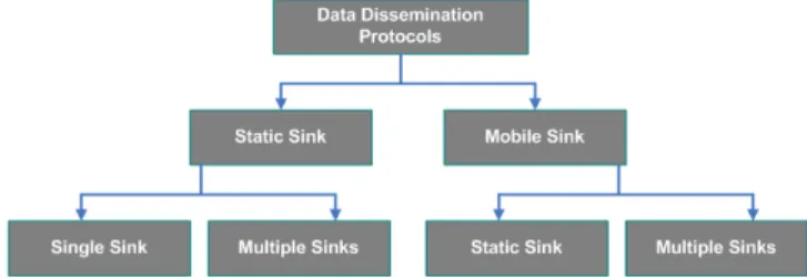
Our classification in this work is mainly based on the number of sink(s) (single or multiple) and their nature (static or mobile). Some protocols require that the sink node has to be static and sensor nodes cannot achieve their requirements without this assumption. Other protocols support the mobile sink concept and try to exploit this possibility to provide a good performance. Moreover, in these kinds of protocols, some use more than one sink which requires additional management and coordination operations.
Figure 1. Taxonomy of data dissemination protocols in wireless sensor network.
Considering these key parameters, we suggest classifying the existing data dissemination protocols according to the taxonomy shown in Figure 1. Two great classes can be found; (i) Static sink data dissemination protocols and (ii) Mobile sink data dissemination protocols. Each class is again divided into two subclasses related to the number of sink(s).
3. Static Sink Data Dissemination Protocols
Sink node in a WSN is the most important entity. The collected sensor readings from sensory field have to be disseminated to a predefined sink for analysis and processing. The data dissemination strategies with single static sink try to prolong the network lifetime by unbalancing
the traffic load using multiple data dissemination paths. Nevertheless, sensor nodes near the sink still deplete their energy faster than that of other nodes due to their heavy overhead of relaying messages. This uneven energy depletion phenomenon causes degraded network performance and limits network lifetime. If all sensors around the sink consume their energy, the sink will be isolated from the network, and then the entire network would fail. Using multiple static sinks can significantly improve the network performance in terms of latency and energy consumption. Having multiple sinks in the network reduces the distance between sensor nodes and a sink, thus can improve both energy consumption and latency [32-37]. A WSN with multiple sinks can be regarded as set of sub-networks, each of which is composed of a single sink. The number and the locations of sinks should be thoroughly studied as they could directly affect the network lifetime [38-41].
3.1 Single Static Sink Data Dissemination Protocols
3.1.1 Low Energy Adaptive Clustering Hierarchy (LEACH)
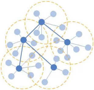
LEACH [42] is the first and most commonly known energy-efficient hierarchical clustering algorithm for wireless sensor networks. LEACH is a cluster-based protocol, which includes distributed cluster formation (Figure 2). LEACH randomly selects a few sensor nodes as cluster-heads and rotates this role to evenly distribute the energy load among the sensors in the network. In LEACH, the cluster-head node aggregates the sensed data arriving from nodes that belong to its cluster, and sends an aggregated data to the base station in order to reduce the amount of information that must be transmitted to the base station.
LEACH process starts with the entire nodes organizing themselves through the clustering algorithm to form a cluster where one node will be elected as a head node or cluster head. Energy will be depleted more if the cluster head is fixed into one node, thus LEACH has the ability to rotate the cluster head among the nodes in the local cluster. LEACH protocol uses aggregation method to gather all information from the sensor nodes in the local cluster where the cluster head will collect the information for sending to the base station. LEACH protocol design can be divided into three different angles:
- Nodes clustering,
- Data gathering for aggregation, - Cluster head rotation.
In node clustering setup, each sensor node will select in which cluster it belongs based on the distance between the node and cluster head. The process needs the cluster head to broadcast a message to all its neighboring nodes which alerts them that it is a cluster head. After receiving all the messages from the nodes that would like to be included in the cluster and based on the number of nodes in the cluster, the cluster-head node creates a TDMA (Time Division Multiple Access) schedule and assigns each node a time slot to transmit its data. This schedule is broadcast to all the nodes in the cluster. This schedule permits the nodes to turn off their transmitters if there is no activity in the cluster. Hence, this mechanism reduces inter-cluster collision and energy consumption.
is being gathered from the sensor nodes in local cluster. The most important part in LEACH cluster head is the way it handles the rotation among the nodes for cluster head elects. Nodes have to elect the head by themselves based on the energy remaining in the nodes and some given probability calculated individually by each node.
Figure 2. LEACH architecture.
Although LEACH is able to increase the network lifetime, there are still a number of issues about the assumptions used in this protocol. LEACH assumes that all nodes can transmit with enough power to reach the base station (BS) if needed and that each node has computational power to support different MAC (Medium Access Control) protocols. Therefore, it is not applicable to networks deployed in large regions. It also assumes that nodes always have data to send, and nodes located close to each other have correlated data. It is not obvious how the number of the predetermined cluster-head is going to be uniformly distributed throughout the network. Therefore, there is the possibility that the elected cluster heads will be concentrated in one part of the network. Hence, some nodes will not have any cluster-head. Furthermore, the idea of dynamic clustering brings an extra overhead, which may increase the energy consumption. In [27], a centralized cluster formation version of LEACH has been proposed, where the base station organizes and controls the network. This protocol provides a centralized cluster formation, local processing for aggregation of sensed data and the rotation of cluster heads for every round. These activities are aimed at achieving uniform energy consumption among sensor nodes and maximizing network lifetime. Since, the base station does not have energy constraint, centralized cluster formation methods can be attractive alternatives. In this protocol [27], the cluster formation is formulated as a p-median problem [43], which is one of the well-known facility location problems (Just to clarify a bit here, the p-median problem can be stated very simply, like this: given a set of customers with known amounts of demand, a set of candidate locations for warehouses, and the distance between each pair of customer-warehouse, choose p warehouses to open that minimize the demand-weighted distance of serving all customers from those p warehouses [44]). This algorithm produces better clusters by dispersing the cluster head nodes throughout the network.
3.1.2 Threshold-sensitive Energy Efficient Protocols (TEEN and APTEEN)
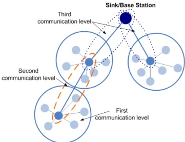
Threshold-sensitive Energy Efficient sensor Network protocol (TEEN) [45], and (Adaptive Periodic Threshold-sensitive Energy Efficient sensor Network protocol (APTEEN) [46] are two hierarchical dissemination protocols proposed for real-time application. In TEEN, the authors assume that base station and sensor nodes have same initial energy and base station can communicate directly with each sensor nodes in the network. In this protocol, the sensor nodes sense their environment continuously, but the transmission is done less frequently. As shown in Figure 3, the network consists of three communication levels: simple nodes communicate directly with their cluster head and constitute the first communication level; then, cluster head can communicate directly with the base station, or via another intermediate cluster head.
Cluster head sends two parameters to its neighbors, hardware threshold and software threshold - the hardware threshold being the minimum value of an attribute permitting a sensor node to power-on its transmitter and transmit to its cluster head. It permits reducing the number of transmissions by allowing a sensor node to transmit its data if the sensed attribute is in the range of interest. The software threshold reduces the number of transmissions which could have differently occurred when there is little or no change of the sensed attribute.
Figure 3. TEEN and APTEEN architecture.
Based on the two thresholds, data transmission can be controlled and reduced which decreases the energy consumption and improves the effectiveness and usefulness of the receiving data. However, in TEEN, a sensor node may waste its time slot if it does not have any data to transmit. Also, cluster head has to keep its transmitter power “on” to receive data from its members; thus, more energy would be consumed.
After creating the clusters and selection of the cluster heads by the base station in each round, the cluster head sends to its member nodes some parameters concerning the physical parameters; the hard threshold and soft threshold values, the time slot to each node using TDMA and the maximum time period between two successive reports sent by a node. In APTEEN, the cluster head aggregates all the data received from its member nodes and sends it to its higher level cluster head or to the base station which allows reducing the network overhead and the overall energy consumption. Moreover, APTEEN is suitable in both proactive and reactive applications. However, this protocol generates an additional cost and more overhead to organize the sensor nodes in complex multiple levels of clusters.
3.1.3 Power Efficient Gathering in Sensor Information Systems (PEGASIS)
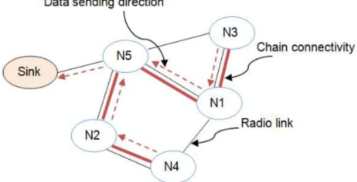
In LEACH [42], each node sends the collected data to its cluster-head, which unnecessarily implies a transmission of a great mass of information and it consumes much energy especially if these data are redundant. PEGASIS [47] is proposed to solve this problem and improve the LEACH protocol. In this protocol, each node communicates only with its nearest neighbor and only one node is selected to transmit to the sink which creates a chain communication shape. The chain is constructed in greedy way by assuming that all nodes have global knowledge of the network. The chain construction is started by the farthest node from the sink (node N3) to ensure that nodes farther from the sink have close neighbors.
Figure 4. Chain construction and data passing approach.
Figure 4 shows a chain example (N3, N1, N5, N2, N4) after executing the greedy algorithm. When a node dies, the chain is reconstructed in the same manner to bypass the dead node. Node N5 presents the chain-head and it is responsible to transmit the gathered data to the sink. The chain-head is equitably rotated among the nodes of the chain. Chain-head is selected randomly, and each node has the chance to be the leader once every N round (N is the number of nodes). For gathering data in each round, the chain-head sends a control packet to its neighbor to start the data transmission from the end of the chain. In Figure 4, node N5 sends this control packet along the chain to node N3. Node N3 will send its data towards node N5. After node N5 receives data from node N1, it will pass the control packet to node N4, and node N4 will pass its data towards node N5 via node N2. Each intermediate node has to aggregate the received data with its local data before sending it to its next neighbor node in the chain. Thus, chain-head sends only one message to the sink by round.
This technique of communication used by PEGASIS allows saving more energy compared to that of LEACH [42] to increase the lifetime of the network and to reduce the bandwidth consumed by using local collaboration between the nodes and by tolerating the failure of the sensor nodes. However, the direct communication between chain-head and sink consumes more energy especially when the distance between them is longer. Moreover, the latency is more important; thus, this protocol cannot be used for real-time applications.
3.1.4 Simple Energy-Efficient Routing (SEER)
SEER’s [48] data dissemination is source-based which eliminates the need for the sink to flood an interest for data through the network. Nodes only transmit data when new data are observed. Data are routed along a single path, which is dynamically established. Every time when a node needs to send data, it selects one neighbor to send the message based on the neighbor’s hop count and available energy.
Once the network has been deployed, the sink transmits a broadcast packet with header field of 64 bits. 16 bits are reserved for node, each node in the network is assumed to have a unique address within the network and the header field contains source and destination node addresses. 8 bits are reserved to identify new broadcast messages using a sequence number. The sink increments the sequence number every time it sends a new broadcast message. Nodes store the sequence number locally and forward the broadcast messages only if the sequence number of the message is different from the stored one. The sequence number permit to avoid redundant forwarding of old broadcast messages. An 8 bit hop count ensures that nodes can be up to 255 hops away from the sink.
When a node receives this initial broadcast message, it checks whether it has an entry in its neighboring table for the node that transmitted the message. If not, it adds an entry that consists of the neighbor’s address, hop count, and energy level. The node then increments the hop count stored in the message and stores this hop count as its own hop count. It then retransmits the broadcast message, but changes the source address field to its address and the energy level field to its remaining energy level. Every node in the network retransmits the broadcast message once, to all of its neighbors. If a node receives a broadcast message with a lower hop count than the hop count it currently has, it updates its hop count. When this initial broadcast has been flooded throughout the network, each node knows its hop count and has the address, hop count, and energy level of each of its neighbors.
Before the message is sent, the remaining energy entry for the selected neighbor is decreased in the neighboring table. If the message is a critical one, a second neighbor will be selected using the same process. Here, using hop count as the routing metric ensures that the message is always sent to the direction of the sink.
When nodes receive a data message, they update the remaining energy value of the sending node in their neighboring table and forward the data using the same dissemination process; the sending node has to be excluded from the list of the neighboring nodes to avoid any routing loop in the network. When a node’s remaining energy decreases than a certain threshold, it transmits an energy message to all of its neighbors to inform them about its energy level.
3.1.5 Energy Aware routing Protocol (EAP)
In [49], authors proposed a novel energy-aware routing protocol (EAP) to prolong the lifetime of sensor networks. EAP introduces a new clustering parameter for cluster head election. As LEACH, EAP is divided into rounds, each round begins by a set-up phase in which clusters are organized and routing tree is constructed, followed by a working phase to collect and send data to the sink node. In EAP protocol, each node needs to maintain a neighborhood table to store the information about its neighbors. Each node located in the cluster range is seen as neighbor. At the beginning of each round, each node broadcasts its residual energy (E) to its neighbors and setup its state as cluster head candidate. Each node receives the residual energy from all the neighbors in its cluster range. Then, accordingly it updates its neighborhood table and calculates the average residual energy (E ) of the cluster range and the broadcasting delay time T using the following equations:
∑
where is the number of neighbors in the cluster range.
T K P ,
where K is a real value uniformly distributed between 0 and 1, and P is the time duration for cluster heads election. During the T time, a sensor waits to receive any proposed cluster head message from its neighbors. If it does not receive any proposition, it proposes itself and broadcasts its proposition to be cluster head to its neighbor nodes. After broadcasting its cluster head proposition, it has to wait 2 ∆t, where ∆t is the time interval which can ensure that all neighbor nodes can receive the cluster head proposition message, to make sure whether there exists another cluster head proposition broadcasted by other nodes in its cluster range. If it does not receive any proposition from its neighbors over ∆t, it sets its state as “Head”, or else, it compares its weight with the weights of other broadcasting neighbors. If its weight is the largest one, it sets its state as Head and other broadcasting neighbors give up the competition. Otherwise, the node sets its state as member sensor of this cluster.
To reduce energy consumption, EAP adopts the same intra-cluster coverage scheme introduced in [50]. This scheme permits the cluster head to choose randomly active nodes to ensure a certain required coverage limit. The remaining
nodes perform as redundant nodes and turn their radios off to minimize energy consumption.
To define the routing tree after clustering (Figure 5), each cluster head broadcasts within a cluster range a weight message, which contains node ID and its weight W defined as below:
D RSS!" E
D RSS# $" E
where RSS! is the node %’s received signal strength for the
signal broadcasted by the base station, RSS# $ is a constant
which is determined by the location of the base station, and the function D is used to estimate the distance between node
% and the base station. After the deployment of sensors, the base station broadcasts probing message to all sensors and sensors acquire the RSS according to the received signal strength. RSS remains constant during the network lifetime unless base station varies its location or sensor nodes are mobile.
The cluster head compares its own weight and the received weight of the other neighbor cluster heads. If it has smaller weight, it selects the node that has the largest weight as its parent and sends a message to notify the parent node. After a specified time, a routing tree is constructed. The root node has the largest weight among all cluster heads in the same independently connected component. The node that is closer to the base station and located in a sub-region with full energy would be the root node of routing tree due to its higher weight. After routing tree construction, cluster heads broadcast a TDMA schedule to their active member nodes to be ready for data gathering.
Figure 5. EAP architecture.
3.1.6 Directed Diffusion dissemination protocol (DD)
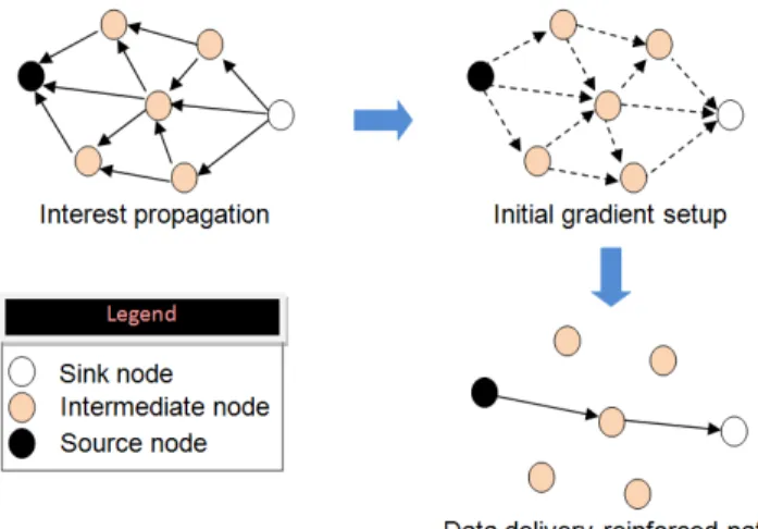
Directed Diffusion data dissemination protocol [53-54] is the first proposed data-centric communication protocol for wireless sensor scenarios. The data generated by the producer is named using attribute-value pairs. Figure 6 shows the operation of data-centric communication protocol. Directed diffusion is based on query, where sink queries the sensors in an on-demand fashion by disseminating an interest. As shown in Figure 6, DD consists of three phases: Interest propagation, initial gradient setup, and data delivery along reinforced path.
In directed diffusion, the data generated by the nodes are named by attribute-value pairs and the data dissemination process is a destination-initiated reactive routing technique in which routes are established when requested.
In the Interest propagation phase, the sink node broadcasts its interest message to all its neighbors. All nodes have an interest table in which the received interest message has to be saved. Each entry in this table has several fields. The most important fields are timestamp field which contains the last received matching interest, gradient fields which contain the data rate specified by each neighbor and duration field which contains the lifetime of the interest. When a node receives an interest, it checks its interest cache to check if it has an entry.
Figure 6. Directed diffusion phases.
It creates one if there is no matching interest and a single gradient field is created towards the neighbor from which the interest is received and forwards the requested interest message to its neighbors. A gradient is removed from its interest entry when it expires. A gradient specifies both the data rate as well as the direction in which the events are to be sent. If the interest exists, the timestamp and the duration fields are updated in the entry and the second step starts. In the initial gradient setup, the sensor node which has a matching interest entry generates event samples and sends an event to all its neighboring nodes for which it has gradients. The last phase begins when the sink starts receiving this event, possibly along multiple paths. The sink then sends a reinforced packet to the neighbor node which is the first one receiving the target data. The neighbor node which receives the reinforced packet can also reinforce and select the neighbor node which can receive the new data first. Consequently, a path with maximum gradient is formed; hence, in future, received data packets can be transmitted along the best reinforced path. Finally, the real data are sent from the source to the sink using the selected path.
3.2 Multiple Static Sinks Data Dissemination Protocols
3.2.1 A Stateless Protocol for Real-Time Communication in Sensor Networks (SPEED)
SPEED [48] is a real-time communication protocol designed for sensor networks. Speed provides three types of real-time communication services namely: real-time unicast, real-time area-multicast, and real-time area-anycast. These communication types are defined as follows.
Real-time unicast. This is “more to one” communication mode which occurs when one part of a network detects some activity that needs to be reported to a remote base station. Real-time area-multicast. Contrary to the first communication type, real-time area-multicast is “one to more” communication mode. This type of communication occurs when the base station initiates the communication by sending its query to an area in the sensor network.
Real-time area-anycast. This communication mode can be used when the response of any sensor node is sufficient. SPEED is specifically customized to be a stateless protocol. That means, it only maintains immediate neighbor information and does not require a routing table. SPEED provides a uniform delivery speed across the sensor network to meet the requirement of real-time applications such as disaster and emergency surveillance in sensor networks. To avoid congestion, SPEED uses a novel backpressure re-routing scheme to re-route packets around large-delay links with minimum control overhead. It also uses non-deterministic forwarding to balance each flow among multiple concurrent routes.
The routing module in SPEED is called Stateless Non-deterministic Geographic For- warding (SNGF) and it works with four other modules at the network layer [55]. Figure 7 shows these different modules.
The beacon exchange mechanism is used to collect information about nodes and their locations. Delay estimation at each node is made by calculating the elapsed time when an ACK is received from a neighbor as the response to a transmitted data packet. SNGF scheme selects nodes that would meet the speed requirement by estimating delay values.
Figure 7. SPEED modules.
performs better in terms of end-to-end delay and miss ratio. SPEED reduces transmission energy consumption, control packet overhead, and traffic distribution. It is also able to achieve load balancing in the network to a great extent. SPEED, although is a successful real-time WSN routing protocol based on simple routing algorithm, it is not really energy efficient. SPEED uses only one delay threshold overall to manage transmission of data packets at the highest transmission velocity. As a result, it cannot satisfy different requirements for transmission delay and causes huge energy consumption.
The protocol indeed results in energy exhaustion of nodes quickly because it selects nodes having high transmission velocity without considering the remaining energy of nodes. Therefore, for a more realistic understanding of SPEED’s energy consumption, there is a need for comparing it to a routing protocol, which is energy-aware.
In addition to these issues, the idea of per-flow reservation appears to be non-scalable in SPEED due to the highly dynamic links and route characteristics. So, SPEED might not be scalable well for large WSNs. There is an extension of SPEED, called FT-SPEED [58], which is proposed to handle the void problem caused by high sensor failure probability in WSN. In FT-SPEED, a “void announce” scheme is designed to prevent packets from reaching the void through other routing paths. It also introduces a void bypass scheme to route the packets around two sides of a void to guarantee that the packets are delivered rather than just being dropped. 3.2.2 Multi path Multi SPEED (MMSPEED)
Multi-path and Multi-SPEED Routing Protocol (MMSPEED) [59], an extension of SPEED is designed to support multiple communication speeds, which provides differentiated reliability. A key feature of MMSPEED is that it addresses both real-time issue and reliability separately. The main goals of MMSPEED design are.
• Localized packet routing decision without global network state update or a priori path setup. • Providing differentiated QoS (Quality of
Service) options in isolated timeliness and reliability domains.
For the first goal, geographic routing mechanism based on location awareness is used. Each sensor node is assumed to be aware of its geographical location. This location information can be exchanged with immediate neighbors with “periodic location update packets”. Thus, each node is aware of its immediate neighbors within its radio range and their locations.
For the second goal, MMSPEED provides multiple delivery speed options that are guaranteed network-widely. For this, the idea of SPEED protocol [48] which can guarantee a single network-wide speed is used. MMSPEED assumes a few important assumptions.
(1) All nodes know their geographical location. (2) Location of the packet destination is known.
(3) The underlying MAC protocol allows prioritizing between different classes at least stochastically.
(4) Each speed level is mapped onto a MAC layer priority class.
Associating messages with deadlines focuses on the problem of providing timeliness guarantees for multi-hop transmissions in a real-time sensor application. In such application, each message is associated with a deadline and
may need to traverse multiple hops from the source to the destination. Message deadlines are derived from validity of the accompanying sensor data and start time of the consuming task at the destination. The protocol reduces deadline misses by scheduling message based on their per-hop timeliness constraints. It supports a probabilistic QoS guarantee by provisioning QoS in two domains -Timeliness and Reliability. QoS differentiation in timeliness is provided through multiple network-wide packet delivery speed guarantees. The scheme employs localized geographic packet forwarding augmented with dynamic compensation, which compensates for local decision inaccuracies as a packet travels towards its destination. The intermediate nodes can lift speed level if they find that the packet may miss the delay deadline with current speed but may meet it at a higher level. To reduce the number of collisions, the QoS has been enhanced in [60] by adapting the Contention Window Adapter (CWA) mechanism in which a dynamic contention window has been used.
In supporting service reliability, probabilistic multi-path forwarding is used to control number of delivery paths based on the required end-to-end reaching probability. In this scheme, each node in the network calculates the possible reliable forwarding probability value of each of its neighbors to a destination by using the packet loss rate at the MAC layer. According to the required reliable probability of a packet, each node can forward multiple copies of it to a group of selected neighbors from the forwarding neighbor set to achieve the desired level of reliability. These mechanisms for QoS provisioning are realized in a localized way without global network information, which is desirable for scalability and adaptability to large scale dynamic sensor networks.
Though, MMSPEED [59] does some improvements over SPEED and differentiates among different real-time levels, it does not dynamically adjust routing paths according to the node’s energy state. Both SPEED and MMSPEED have a common deficiency that is they do not take into account the energy consumption metric. This metric has been considered by EAMMSPEED protocol [61] which tries to balance the load and energy consumption of individual nodes in the network and improve the overall network lifetime. Therefore, each node makes routing decisions based on the following four parameters: geographic progress towards the destination sink, required end-to-end total reaching probability, delay, and residual energy at the candidate forwarding node. The performance evaluation shows that EAMMSPEED protocol provides stable service in the sensor network and maximizes the lifetime of the entire network while maintaining the QoS guarantees provided by MMSPEED.
3.2.3 Sequential Assignment Routing (SAR)
SAR [62] is the first protocol for WSN-oriented QoS. SAR calculates multiple paths from the source nodes to the sink, by building trees rooted from a 1-hop neighbor from the sink (Figure 8) and growing outward until it reaches leaf nodes while avoiding paths with low energy or low QoS guarantees. At the end of this process, each leaf node would belong to multiple trees and thus, would have multiple paths to reach the sink.
(1) Energy resource estimated by the maximum number of packets that can be routed before all of the energy is depleted.
(2) Additive QoS metric, where higher metric implies lower QoS.
Each node generating packets makes a decision about which path to choose. This decision is based on the energy resource and a weighted QoS metric which is the additive QoS metric multiplied by a weight coefficient associated with the priority level of the packet.
SAR shows an optimized performance focusing on lowering of the energy consumption of each packet without considering its priority. A routing table update revolves around the network so as to update all the routing tables of the network in order to find out the depleted nodes in the network and ignore any further communication through the ruined path.
Figure 8. SAR architecture.
The objective of the SAR algorithm is to maximize the lifetime of the network while minimizing the average weighted QoS metric. One of the drawbacks of this protocol is the high overhead due to the large number of tables being kept on each node, especially when the number of nodes becomes huge.
3.2.4 Hierarchy-Based Multipath Routing Protocol for Wireless Sensor Networks (HMRP)
In HMRP [63], sensor nodes are assumed to be fixed for their lifetimes, and the identifier of sensor nodes is determined a priori. Additionally, these sensor nodes have limited processing power, storage and energy, while sink nodes have powerful resources to perform any task or communicate with the sensor nodes.
HMRP is based on the hierarchical tree architecture, in which the sink nodes serve as root nodes. Each sensor node must be a member of the architecture. The protocol has two phases: Layer Construction Phase (LCP) and Data Dissemination Phase (DDP).
In the first phase, HMRP forms hierarchical relations by broadcasting a network construction packet (NCP) to all its neighbors. This packet contains Seq_Number, Hop_Count, Source_ID, Sink_ID, Packet_Type. The sink node initiates the Hop_Count by one, updates the other fields and broadcasts the packet with Layer Construction Request type to discover the one hop nodes. Each sensor node that receives this packet compares the Hop_Count field with its hop value in its routing path formation table. If Hop_Count field is smaller than its own hop value, then it keeps the
packet during some period and updates its routing path formation table, else it drops the packet. If the time of the period duration is finished, the node selects the Source_ID of the received packets with the lowest Hop_Count values as its candidate parents. If the node receives more packets with the same lowest Hop_Count, it saves all Source_ID of the received packets as its candidate parents. This node then updates the Hop_Count and the Source_ID fields in the packet and rebroadcasts it again. Every node continues flooding the Layer Construction Request type packet until the network level is constructed.
In the second phase, Sensor nodes can start disseminating the sensed data to the sink via the parent node. A Received Data Acknowledge (RDACK) packet is sent when the data packet is successfully transmitted to the parent node. The parent node then replies with this packet to notify the source node, and forwards the data packet to next hop. In case of several parents, the source node chooses the parent node as next hop using Round Robin Scheduling when it wishes to send a data packet to a sink. When the source node receives an ACK from the selected parent, it moves this record of this parent in its routing path formation table to the last position and transfers the data packet to the next parent. If no ACK reply is obtained from the parent during some period of time, the source node deletes the record of the concerned parent from its routing path formation table.
The main advantage of HMRP is that the sensor node needs only to know to which parent node to transfer, without maintaining the whole path information. This can reduce the overhead of sensor node. Furthermore, HMRP supports multipath data forwarding path which distributes the energy and prolongs the lifetime of network. However, this protocol has some weaknesses like using an ACK to notify the reception of each data packet increases the network overhead and consumes energy too. This information can be recorded from MAC layer. Moreover, HMRP supports multiple sink nodes scenario, but it does not specify any sink node management procedure - in fact, sink nodes work without any coordination among them, and thus, it has an impact on the overall network performance.
3.2.5 Sinks Accessing data From Environment (SAFE)
SAFE [64-65] is a data dissemination protocol for wireless sensor networks. In this protocol, sensor node can disseminate its sensed data to sinks that explicitly present their interests by sending data requests. Each data sink is allowed to specify its own desired data update rate. SAFE has two major phases: query transfer and dissemination path setup.
In query transfer phase, user sends -via sink node- its query specifying the location, the sensor data type, the desired data update rate, and the service duration. Every node maintains a recent query table and a data management table. The query table records the most recent queries that have been received, and the data table keeps the status of sensor data being or to be distributed by the node. Each node that receives the query performs the tasks as noted below.
• Check the query table if the same query has recently been dealt with. If so,
• Ignore the new query, Otherwise, • Save the query into its query table
the source but on a dissemination path, which is called a junction node, it sends a JunctionInfo message to the sink via unicast. When the node is neither the data source nor a junction, it forwards the query to the next hop, as long as it is not farther away from the queried location than the previous hop node. The hop sender information might be extracted from the packet header filled by the routing protocol in use, or injected by this data dissemination protocol before forwarding a query.
In the second phase of dissemination path setup, each intermediate node has already inserted the necessary information in its data management table while receiving the PathSetup message during the last phase. The intermediate node sets a timer for waiting an Ack message from its descendant, which confirms the path is activated. When the sink node receives the PathSetup and the JunctionInfo messages, it waits for a certain amount of time and then subscribes to the node that sent the best feedback until then. If the best one is a junction node, the sink sends a Subscribe message to this node. When junction node receives this message, it sends a TrailSetup message to that sink and establishes the dissemination path. Otherwise, when the source is eventually the best subscription point, the sink sends an Ack to its progenitor and every progenitor acknowledges its progenitor in turn until the source gets an Ack message and establishes the dissemination path.
4. Mobile Sink Data Dissemination Protocols
Mobile sink wireless sensor network has recently attracted a lot of attention from the research community. Recent works [66-72] have shown that the use of mobile sink can enhance connectivity and lifetime of WSNs. Mobility has been proposed as an alternative way in the literature for reducing the communication distance between sensor nodes and sinks. Network lifetime can be improved with mobile sinks by reducing multi-hop communication and avoiding the bottleneck problem, which appears on the nodes close to the static sink.
In wireless sensor networks, mobility can appear in three main forms [73]: mobility of the sensor nodes that sense the environment and transmit the sensing data, mobility of sinks that gather the information from the network and forward data to the applications, and mobility of the observed event. Sinks can adopt mobility schemes according to the nature of WSN application and its requirements. This mobility can be classified into three categories [66].
(1) Uncontrolled or Random Mobility [74-77]. (2) Predictable Mobility [70], [78-79]. (3) Controlled Mobility [66], [68-69], [80]. 4.1 Single Mobile Sink Data Dissemination Protocols
4.1.1 Congestion Avoidance Energy Efficient routing protocol (CAEE)
In [81], the authors tried to solve the problems of data loss due to congestion around the static sink, and the high energy consumption of the sensor nodes located in the vicinity of the static sinks. Therefore, the authors present a routing protocol that is based on an in-network storage model [82], and a mobile sink.
In an environment where the sensor nodes are uniformly but randomly deployed, the authors assume the following points. • Sensor nodes are grouped into clusters, where
cluster head is designated for each cluster.
• Cluster head forwards the received data from neighboring head nodes and the nodes of its cluster towards the sink.
• Depending on the node density and sensor field coverage requirements, the cluster head manages the nodes of its cluster by assigning them “awake” or “sleep” status.
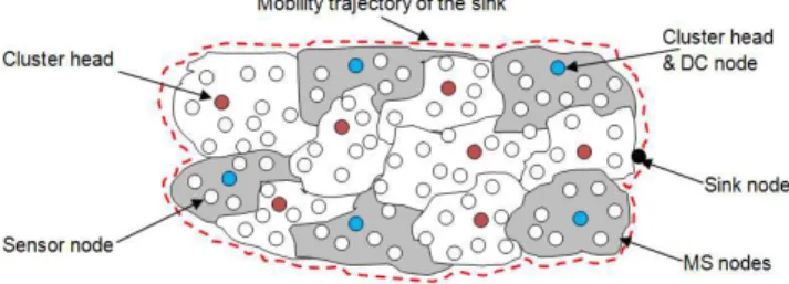
• Each node has a list of all its neighboring nodes. CAEE is based on discrete sink mobility along a fixed trajectory. In CAEE, Mini-sinks (MS) are created utilizing the in-network storage model [82] along the mobility trajectory of the sink. Each MS (Figure 9) is considered as a cluster of sensor nodes managed by cluster head called a data collector node (DC). The DC node receives the collected data from the sensor field and stores it in the MS nodes. The mobile sink periodically visits each MS and retrieves the stored data.
The CAEE protocol does not impose any restriction on the shape of the mobility trajectory of the sink. The mobility path of the sink is along the periphery of the sensor field. During its first trip along the periphery of the sensor field, the sink selects a subset of sensors as DC nodes. Each DC node sets up its MS, and broadcasts this information to the sensor nodes. The sink node starts its first mobility round along the periphery of sensor field to select the DC nodes. It chooses the first or the starting node as DC1 if the last one is cluster head. Otherwise, the sink queries the start node about its cluster head node. On retrieval of the required information, the sink assigns the status of DC1 to the obtained cluster head node. Thus, the sink starts its mobility along the periphery of the sensor field, and selects the second data collector node DC2 that is located at least H hops away from DC1. Similarly, the third data collector node DC3 is located at least H hops away from DC2, and so on. In this way, a set of DC nodes are created along the periphery of the sensor field.
To create the MS nodes, each DC node broadcasts a message to invite the sensor nodes to joint its K-hop cluster. The message contains the ID of the DC node and the hop count that is initialized with 1. Each sensor node receiving this message does the following tasks:
• Compares the available routing path to a data collector node with the newly reported route and keeps the shortest one.
• Increments the hop count by 1 in the received message and forwards it.
After a certain period of time, each node knows a shortest possible route to one of the data collector nodes as shown in Figure 9.
Figure 9. CAEE architecture.
In this protocol, the collected data from the sensor node to the MS node are transmitted over the shortest path which increases the lifetime of the network. Also, congestion and data delivery delay have been improved because of the mobility of sink and the multiple MSs. However, this protocol may suffer from latency which can be increased as the number of MSs in the network increases. Hence, this protocol is not recommended for a large scale sensor network and real-time applications.
4.1.2 Sink Mobility Protocols for Data Collection (SMPDC)
Sink mobility has been investigated as a method for efficient and robust data delivery in wireless sensor networks [83], [84]. The authors proposed four mobility patterns for the sink, mostly randomized (such as the simple random walk, biased random walks, and walks on spanning sub graphs), as well as predictable mobility (moving on a straight line or cycle). These patterns assume and exploit different degrees of freedom, simplicity and network knowledge. To get data from sensors, the sink movement is combined with three data collection strategies: a passive, a multi-hop, and a limited multi-hop.
The authors consider an environment composed of a huge number of small homogeneous sensor devices with limited capabilities. They suppose that the sensor devices are randomly deployed in a flat square area. The sink does not have any resource limitation, it can calculate accurately its position using Global Positioning System (GPS) and it is aware of the dimension of the network area.
The first proposition called Random Wall and Passive Data Collection (RWPDC) is a simple mobility pattern in which the mobile sink moves randomly towards a chosen direction with constant speed. The mobile sink selects a random uniform angle in [&π, π] radians. This angle defines the deviation of the mobile sink’s current direction. To determine the new position, the mobile sink selects a uniform random distance d * 0, dmax" which is the distance to travel along the newly defined direction. If the new position is outside the network area, the sink decreases the distance to the network area border. The data are collected in passive manner. The sink broadcasts periodically a beacon message. Each sensor node that receives this message replays by transmitting its data to the sink. RWPDC presents the simplest possible movement, guarantees visiting all sensors in the network, and thus, collects data even from disconnected areas in case of few/faulty sensors or in the presence of obstacles. However, the latency is the biggest problem of this method.
The second proposition is called Partial Random Walk with Limited Multi-hop Data Propagation (PRWLMDP). In this proposition, the authors assume that the network area is partitioned as equal square regions. The center of each region
is connected to the center of the adjacent regions. Initially, the mobile sink is positioned on or near one of the center nodes. Then, it calculates the next position by selecting randomly one of the neighbors of the current center. Thus, the sink moves toward this new position with predefined constant speed.
The data collection protocol forms propagation trees. The sink periodically broadcasts a beacon message and indicates the depth of the propagation trees by setting a TTL (Time To Live) parameter. This process creates a number of propagation trees within the network with the roots of these trees being one hop away from the sink. Sensor nodes that belong to propagation tree may begin immediately forwarding their data to the sink.
As the sink moves on, the propagation trees may become disconnected. When the root node loses the communication with the sink, it simply caches all data both generated and relayed, and waits to hear another beacon message to begin the propagation process again.
In this scheme, the distance traveled by the sink is reduced and the time to visit network nodes is accelerated. However, PRWLMDP uses more knowledge of the network which is more expensive in terms of communication and computational costs on the sensor devices.
The third proposition called Biased Random Walk with Passive Data Collection (BRWPDC) extends the previous one (PRWLMDP). The authors use the same assumptions and the same data collection protocol. In this proposition, the sink calculates its next position based on two parameters: the visiting frequency of the region and the number of sensor nodes in the region. The center of the region that has the low visiting frequency and the high number of sensor nodes will be selected as the next position to move toward it. The low visiting frequency is preferred to speed up the coverage of new areas. To increase data delivery in areas with many nodes, the region of high number of sensor nodes is preferred.
The last proposition is called Deterministic Walk with Multihop Data Propagation (DRWMDP), in which the sink’s movement is predefined. The trajectory is characterized by its length (L). The authors use a particular trajectory (line or circle trajectory). The linear trajectory consists of a horizontal or vertical line segment passing through the center of the network. The sink moves from one edge of the line to other and returns along the same path. The circle is centered at the center of the network and its radius is defined as /
0
12. Initially, the sink is positioned on the perimeter of the
circle and continues along this path. In this kind of sink mobility, the authors use a data collection protocol similar to the one presented in the second proposition (PRWLMDP), without the timeout and TTL mechanism, thus paths are created according to minimum hop distance and span throughout the whole network area. The deployment of this protocol imposes a high cost on the sensor devices that perform tree formation and multi-hop propagation. However, it seems that the delivery latency is lower than any of the three previous propositions. Furthermore, the selection of the trajectory length introduces a trade-off between the cost at the sink and the cost at the sensors.
is important, the second proposition is more appropriate. For the applications where the mobility capabilities of the sink are limited but can tolerate some loss of information and increased energy consumption, the last proposition is more suitable.
4.1.3 Density-based Proactive Data Dissemination Protocol (DEEP)
In [85], the sensing data are proactively distributed and stored throughout the network. The mobile sink is free to choose its own trajectory in any way and at any time. The only condition imposed on the mobile sink in order to retrieve a representative view of the monitored data is on the total number of nodes the mobile sink needs to visit. In DEEP, data dissemination strategy uses a combination of density sensitive probabilistic forwarding with deterministic corrective measures, as given in [86].This technique permits to ensure a predefined average number of transmissions and retransmissions of each message. Based on calculated probability, each node can decide to broadcast any message after receiving it for the first time. If the node does not decide to retransmit the message, it should wait for a given delay and if it does not receive this message from any of its neighbors, then this node retransmits the message. Moreover, in this protocol, the node can store the received message based on another calculated probability.
The simulation results show that DEEP [85] is the more viable solution, especially for sparse networks, when the frequency of sending messages is low, and when the amount of sensed data reported in each message is large. However, the simulation results illustrate that the data storage is well distributed in the network.
4.1.4 Data Collection with Adaptive Stopping Times (DCAST)
In this protocol, the authors propose biased sink mobility with adaptive stop times, as a method for data collection in wireless sensor networks [87-88]. The system model contains a single mobile sink and a vast number of ultra-small homogeneous static sensor devices. Each sensor is a fully-autonomous computing and communication device, characterized mainly by its limited power supply. The sensors are deployed randomly in flat square area. The authors assume the existence of some regions, called pockets, in the network with high sensor node density. Each pocket represents a circular area and does not overlap with another pocket. Moreover, the authors suppose that the mobile sink is not resource constrained. This sink is assumed to be powerful enough in terms of computing, memory, and energy supplies. The sink can accurately calculate its position using GPS and it is aware of the dimensions and the boundaries of the network area. Also, it moves with constant speed according to a given mobility function. The mobility function can be invoked at anytime even before reaching the designated point.
As shown in Figure 10, the network area is partitioned, during the network initialization, as equal square regions, called cells. The center of each cell is connected with unidirectional edges only to the four centers corresponding to adjacent cells.
Figure 10. CAEE architecture.
Thus, when the sink is located at the center of a cell, it can communicate with every sensor node within the cell area. The sink collects the data in a passive manner and broadcasts beacon messages within the cell. Nodes that receive a beacon start transmitting the data stored in their memory to the sink. Initially, the mobile sink is positioned on one of the central nodes. In the Figure 10, two sink mobility schemes proposed by the authors: deterministic walk and biased random walk are represented by the blue-thin and the red-thick arrow lines respectively.
In the deterministic walk, the sink visits cells from left to right and vice versa according to the blue-thin arrow. By moving on this trajectory, the sink can communicate with each node in the network. This walk assumes some global network knowledge to know the boundaries of the cells and the network. It avoids visit overlaps and multi-hop communication, which optimizes the time needed to cover the network. However, in this kind of walk, it may not be feasible to traverse the network with the presence of obstacles that may hinder the movement of the sink. Also, the network topology may not be known to the sink or may change dynamically. To avoid these inconveniences, the authors proposed the second sink mobility scheme (biased random walk) represented by the red-thick arrows in the Figure 10.
In this walk, the next position of the sink is determined by selecting the center of one of the neighboring cells. A frequency is associated with each cell - the sink increases this frequency for each visit to the corresponding cell. The selection of the next area to visit is done in a biased random manner depending on this frequency and the less frequently visited regions are favored.
4.2 Multiple Mobile Sinks Data Dissemination Protocols
4.2.1 Coordination-based data dissemination protocol for wireless sensor network (CODE)
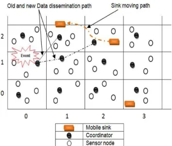
CODE [89] considers energy efficiency and network lifetime, especially for sensor networks with high node density. In this protocol, all sensor nodes are stationary except the sinks nodes. The authors assume that each sensor is aware of its residual energy and its location using the Global Positioning System (GPS) [90]. As shown in the Figure 11, the sensor network field in CODE is divided into grids. Each grid is indexed based on its geographical location. During the data dissemination process, each grid participates by only one coordinator node. The other sensors remain in the sleeping mode using GAF (Geographical Adaptive Fidelity) protocol [91]. The coordinator acts as an intermediate node to cache and relay data.
CODE has two major phases: query transfer phase and data dissemination phase. For example in Figure 11, if an event is detected (grid [1, 0]) the source generates a data-announcement message and sends the message to all coordinators using a simple flooding mechanism. Then, the interested sink sends a query (query transfer phase) to the source node along the path [2, 2] [1, 1] [1, 0] which will be used to transport the sensing data during the data dissemination phase. However, the sink checks its geographical location periodically. If the sink moves out of the grid (from [2, 2] to [2, 1]), it has to send a message to remove the previous data dissemination path and then re-sends a query to set up a new one ([2, 1] [1, 0]).
CODE establishes a better data dissemination path based on the grid ID without flooding and additional phase. The sinks do not need to periodically propagate their geographical location to the sources. Moreover, CODE takes into account query and data aggregation to reduce the amount of data transmitted from multiple sensor nodes to sinks. However, the random sink mobility presents the major inconvenience of this protocol. The mobile sink can move at anytime, goes away from the source node. Thus, it may increase the latency and energy consumption.
Figure 11. CODE architecture.
Figure 12. TTDD structure.
4.2.2 Two-Tier Data Dissemination Protocol (TTDD)
This protocol [77] provides data delivery to multiple mobile sinks based on a decentralized architecture. TTDD uses homogeneous sensors and assumes that each sensor is aware of its own location using GPS [90]. TTDD is grid-based structure. A virtual grid should be created at any new sensed data by the source node. As shown in Figure 12, when the source (S) senses new data, it calculates the locations of its four forecasted neighboring dissemination points (D) based on its geographical position and cell size. The source node then sends a data-announcement message to these neighbors to select the real four dissemination nodes (D). Each dissemination node resends the data-announcement message with the same manner until the construction of the virtual grid as shown in Figure 12.
Instead of broadcasting the location information of mobile sinks to all sensor nodes, TTDD uses a two-tier data dissemination model to deal with the sink mobility problem and reduces energy consumption.
Only sensors located at a cell boundary need to forward the data. The sink proactively builds the two-tier grid structure throughout the network and sets up forwarding points in the sensors closest to the dissemination nodes. The lower tier is the cell at the sink's current location and the higher tier contains the dissemination nodes at cell boundaries. The sink broadcasts its query within its own cell. When the nearest dissemination node in the cell receives the query, it forwards it to its adjacent dissemination node in another cell. This process continues until the query reaches the source node or one of the dissemination nodes that have the corresponding data. During the query propagation, the network establishes the reverse path towards the sink so that the data could be forwarded on the same path as that of the query propagation. TTDD exploits local flood within a local cell of a virtual grid which sources build proactively. However, it does not optimize the path from the source to the sinks. When a source communicates with a sink, the restriction of grid structure may increase the length of a straight-line path. Also, TTDD creates new virtual grid for each new data source. It therefore, increases energy consumption and connection loss ratio. Moreover, sink mobility in this protocol has random scheduler like CODE [89] which affects negatively on the network performance.
dissemination node is selected based on its residual energy. Hence, it can be replaced by another one when its energy becomes equal to the predefined energy threshold. Moreover, EGDD network model ensures query and data forwarding through the shortest path between source and sink. However, sink mobility in this protocol is uncontrolled which brings other challenges for this protocol.
4.2.3 Pseudo-Distance Data Dissemination protocol (PDDD)
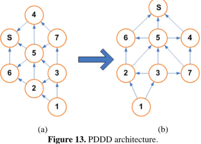
In PDDD [93], network partitioning is not considered and mobile sink nodes are assumed to have unlimited battery power. Also, it is assumed that the links between sensor nodes are bidirectional and no control messages are lost. The main idea of this protocol is to create and maintain a Totally Ordered Graph (TOG) using pseudo-distance. As depicted in the Figure 13(a), when a sink node (S) wants to collect data from sensor nodes, it broadcasts an interest message. By receiving this message, each node can set its pseudo-distance and corresponding level from the sink, and then it broadcasts the received interest message to its neighbor nodes with its own level metric. At the end of this operation, the hierarchical levels of communication are created (Figure 13 (b)). Thus, each sensor node uses this TOG to disseminate the requested data.
Mobile sink nodes generate periodical heartbeat messages to their direct neighbors. Therefore, if the mobile sink nodes move, the direct sink’s neighbors can detect the sink mobility by losing the heartbeat messages. For the other sensor nodes, PDDD uses ACK packet. Each sensor node that transmits data packets to its next hop should receive an ACK from the latter one. If it is not the case, then the link is considered as failed link. Therefore, the sensor node has to choose another redundant path. However, if a node loses all of its parent nodes, then it has to update its own level locally to find new parent.
(a) (b) Figure 13. PDDD architecture.
This protocol can achieve an acceptable data dissemination level in stable sensor network. However, PDDD needs many control messages (interest, heartbeat and ACK messages) to create and maintain the TOG graph. The number of control messages increases when the number of mobile sinks increases. Thus, this fact affects directly and negatively on the network performances like latency and energy consumption. Also, PDDD did not consider the energy parameter in its data dissemination process. Some nodes may be more soliciting than others which would accelerate the death of these nodes. Moreover, like CODE [89] and TTDD
[77], PDDD did not give any strategy of sink mobility which is still random and uncontrolled.
4.2.4 Topology-based Rendezvous Data Dissemination (TRDD)
This protocol [94] assumes a network model of three tiers. Sensor nodes are deployed randomly in the lower tier, each sensor is assumed to be aware of its geographical position using GPS [90]. Sink nodes are placed randomly on the periphery and they constitute the middle tier. The higher tier represents the administration site. TTDD consists of two phases: the events propagation phase and query propagation phase. The dissemination structure of TRDD is based on a simple geometric idea. It considers the network perimeter as a polygon that provides a closed region for the interior nodes called query region (QR). TRDD adapts a modified version of the algorithm presented in [95] to identify dynamically the outer boundary nodes. As shown in Figure 14, the construction of the QR starts once the sinks receive the query from the management site and after discovering the boundary nodes. Thus, QR contains the sensor nodes of the network perimeter and their one-hop neighbors.
When the sensor nodes of one-hop neighbors of the boundary nodes in the QR region receive the query packet, a beacon packet has to be transmitted by those nodes. This beacon allows interior nodes located outside QR to update their neighbor table, to be informed about the creation of the QR region, and to start sending their sensing data toward the QR. After selecting a direction’s path (TRDD proposed eight possible directions) based on three policies: Random-based, Round Robin-based or centroid-based, sensor node selects its closest next hop in this direction. In the first policy, sensor node randomly selects one direction. In the second policy, sensor node selects its direction in order after selecting the first one randomly.
In the last policy, sensor node calculates its position relative to the virtual gravity center of the network and selects the contrary direction relative to this center. Intermediate nodes use the same direction chosen by the initiator node except in failure case, where the intermediate nodes should change the direction. Thus, the sensed data will intersect the QR region and will be transmitted in the reverse path to the root sink. In TRDD, the authors consider and evaluate two sink mobility patterns: random and controlled mobility. In the controlled mobility, sinks move along the network diagonal or along the network periphery.