MICRORHEOLOGY AND HETEROGENEITY IN BIOLOGICAL FLUIDS: APPROACHES, MODELS AND APPLICATIONS
John William Ryckman Mellnik
A dissertation submitted to the faculty of the University of North Carolina at Chapel Hill in partial fulfillment of the requirements for the degree of Doctor of Philosophy in the Curriculum for Bioinformatics and Computational Biology.
Chapel Hill 2015
©2015
ABSTRACT
John William Ryckman Mellnik: Microrheology and Heterogeneity in Biological Fluids: Approaches, Models and Applications
(Under the direction of M. Gregory Forest)
Fluids play an important role in a wide range of biological processes. They facilitate cellular activities, protect us from infection and propagate nutrients throughout the body, to name a few. In each case, the properties of the fluid are finely tuned to the task at hand, and understanding those properties can afford a deeper understanding of the underlying biology. Furthermore, knowing how disease or environmental factors alter the properties of these fluids can provide a means to interpret, and forecast, downstream deleterious effects.
To this end, microrheology is an increasingly popular means of investigating biological fluids. This technique, whereby tracer particles are embedded in the fluid of interest and their diffusive movements are used to infer the viscous and elastic moduli of the surrounding fluid, offers insight into properties of the fluid at a spatial and temporal resolution unmatched by traditional macrorheology approaches.
To my family, past and present
William D. Ryckman, Jr. 1924 – 2003
ACKNOWLEDGEMENTS
This work represents a small facet of a much broader research effort, and would not have been possible without the collaborative spirit, and scientific selflessness, that I have encountered during my seven years at Carolina. It is to those individuals, male and female, whose names I do not know, who established this culture long before I came along, that I would like to offer thanks.
Few people have done more to uphold this culture than the individuals with whom I have been fortunate enough to work, and so, I would like to sincerely thank Paula Vasquez, who introduced me to this research, and David Hill, who introduced me to its applications. I would like to thank Martin Lysy, for his infectious enthusiasm, and Scott McKinley, for his thoughtful guidance. I am thankful for the opportunities afforded by my adviser, Greg Forest, who, despite me, has always demonstrated the most prolific patience and offered the most sage advice.
Early lessons often stick with us the longest, growing as we grow, and so I would like to thank Keith Hale and Mark Aspland, exemplar Corinthians.
CONFLICT OF INTEREST DISCLOSURE
TABLE OF CONTENTS
LIST OF TABLES . . . xi
LIST OF FIGURES . . . xii
LIST OF ABBREVIATIONS AND SYMBOLS . . . xv
1 Introduction . . . 1
1.1 Rheology . . . 1
1.1.1 A brief introduction to micro and macrorheology . . . 2
1.1.2 Generalized Stokes-Einstein Relation . . . 3
1.2 Motivations and objectives . . . 5
1.3 Overview . . . 7
2 Brownian Diffusion Models and Simulation Algorithms . . . 9
2.1 Introduction. . . 9
2.2 Standard Brownian motion . . . 10
2.3 Weyl fractional Brownian motion . . . 11
2.3.1 Theory . . . 11
2.3.2 Simulation techniques . . . 13
2.3.2.1 Direct algorithm . . . 13
2.3.2.2 Frugal Cholesky updates . . . 13
2.3.2.3 Hypergeometric Discrete algorithm . . . 15
2.4 Riemann-Liouville fractional Brownian motion . . . 17
2.4.1 Theory . . . 17
2.4.2.1 Direct algorithm . . . 18
2.4.2.2 Exact Discrete algorithm . . . 19
2.4.2.3 Improved Discrete algorithm . . . 20
2.5 Multi-fractional Brownian motion . . . 25
2.5.1 Theory . . . 25
2.5.2 Simulation techniques . . . 25
2.6 Amnesiac Brownian motion . . . 28
2.6.1 Theory . . . 28
2.6.2 Simulation Techniques . . . 31
2.6.2.1 Path Splicing . . . 31
2.6.2.2 Modified Discrete Algorithms . . . 32
2.7 Local estimations ofH . . . 33
2.8 Conclusion . . . 36
3 Dealing with Drift . . . 38
3.1 Introduction. . . 38
3.2 Mean squared displacement. . . 41
3.3 Fractional Brownian motion and drift . . . 47
3.4 Simulation design . . . 47
3.5 Approaches to parameter estimation . . . 48
3.6 Results . . . 51
3.6.1 Simulated data . . . 51
3.6.2 Experimental data . . . 59
3.7 Conclusion . . . 61
4 Methods for the Quantification of Heterogeneity . . . 63
4.1 Introduction. . . 63
4.2 Current metrics to detect heterogeneity in PPTM data . . . 66
4.2.2 Stage 2 metrics for decomposition of paths into clusters . . . 69
4.3 Materials and methods. . . 70
4.3.1 Materials . . . 70
4.3.2 Particle tracking . . . 71
4.4 Mathematical protocol. . . 71
4.4.1 Calculation of displacements and standard deviations of individual step size distributions . . . 72
4.4.2 Determining the number of clusters. . . 72
4.4.2.1 Hierarchical cluster . . . 73
4.4.2.2 Optimal number of clusters and the gap statistic . . . 73
4.4.2.3 Cluster refining . . . 79
4.4.3 Cluster distribution fitting . . . 79
4.4.4 Algorithm to simulate numerical data . . . 81
4.4.5 Metric comparison. . . 81
4.5 Results and discussion . . . 82
4.5.1 Homogeneous data: simulated and experimental . . . 82
4.5.1.1 Newtonian paths and data analysis . . . 82
4.5.1.2 Viscoelastic paths and data analysis . . . 86
4.5.2 Heterogeneous data: simulated and experimental . . . 89
4.5.2.1 Newtonian paths and data analysis . . . 89
4.5.2.2 Viscoelastic paths and data analysis . . . 93
4.6 Conclusions. . . 99
5 First Passage Times . . . 102
5.1 Introduction. . . 102
5.2 Theory . . . 103
5.3 Simulations and analysis. . . 105
5.4 Results . . . 109
6 Analysis of Pediatric Bronchoalveolar Lavage
Samples . . . 113
6.1 Introduction. . . 113
6.2 Materials and methods. . . 115
6.2.1 Sample collection . . . 115
6.2.1.1 HBE Mucus . . . 115
6.2.1.2 AREST CF . . . 116
6.2.2 Particle tracking . . . 116
6.2.3 Initial path filtering . . . 116
6.2.4 The Background Fluid Problem . . . 118
6.3 Results . . . 127
6.3.1 HBE data . . . 127
6.3.2 AREST CF data . . . 128
6.4 Conclusion . . . 134
LIST OF TABLES
4.1 Sensitivity test of existing heterogeneity metrics . . . 77
4.2 Cluster results for the NGHN data set . . . 81
4.3 Cluster results for simulated homogeneous Newtonian data . . . 83
4.4 Cluster results for experimental homogeneous Newtonian data . . . 83
4.5 Cluster results for simulated homogeneous viscoelastic data . . . 86
4.6 Cluster results for experimental homogeneous viscoelastic data . . . 86
4.7 Cluster results for simulated heterogeneous Newtonian data . . . 89
4.8 Cluster results for experimental heterogeneous Newtonian data . . . 90
4.9 Cluster results for simulated heterogeneous viscoelastic data . . . 94
4.10 Cluster results for experimental heterogeneous viscoelastic data . . . 94
4.11 Cluster results for experimental agarose data. . . 95
4.12 Cluster results for experimental 2.5wt% mucus data . . . 95
6.1 Comparison of the diffusive properties of BAL-derived data points to the expected parameter values based on the background fluid. . . 120
6.2 Cluster results for pediatric bronchoalveolar lavage samples from the AREST CF study with Background Fluid Points . . . 124
6.3 Cluster results for pediatric bronchoalveolar lavage samples from the AREST CF study without Background Fluid Points. . . 125
6.4 Cluster results for 1µm diameter particles in 2.5 wt% HBE mucus . . . 127
6.5 Cluster results for 1µm diameter particles in 3 wt% HBE mucus . . . 127
6.6 Cluster results for 1µm diameter particles in 4 wt% HBE mucus . . . 127
LIST OF FIGURES
2.1 Cholesky weights of three paths forH = 0.1, H = 0.3andH = 0.5
based on the W-fBm covariance . . . 14
2.2 Comparison of weights for the Direct and Hypergeometric Descrete W-fBm algorithms . . . 16
2.3 Weights for threeN = 500step paths generated via the Exact Discrete RL-fBm algorithm. . . 19
2.4 Comparison of weights for the Improved and Exact Discrete RL-fBm algorithms. . . . 20
2.5 Comparison of weights for the Direct, Exact Discrete and Improved Dis-crete RL-fBm algorithms . . . 22
2.6 Comparison of position processes from the W-fBm and RL-fBm algorithms . . . 23
2.7 Comparison of position processes from the W-fBm and RL-fBm algo-rithms, inset. . . 24
2.8 Example mBm path . . . 26
2.9 Illistration of diffusion through a spatially heterogeneous fluid . . . 30
2.10 Comparison of aBm and mBm position process. . . 30
2.11 Example aBm path with sinosodialHgenerated using a modified Improved Discrete algorithm . . . 33
2.12 Local estimates ofHfor an aBm process withHvarying sinosodially. . . 35
2.13 Local estimation of an aBm process with variableDandH. . . 36
3.1 Pathwise MSD for simulated Brownian and subdiffusive particles. . . 43
3.2 Impact of drift-subtraction on the distribution of displacements and MSD.. . . 44
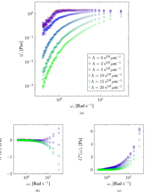
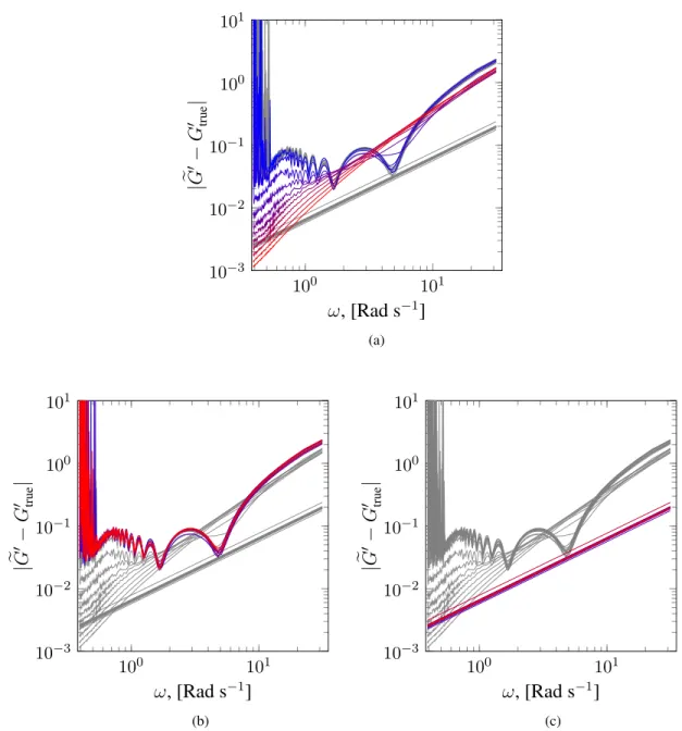
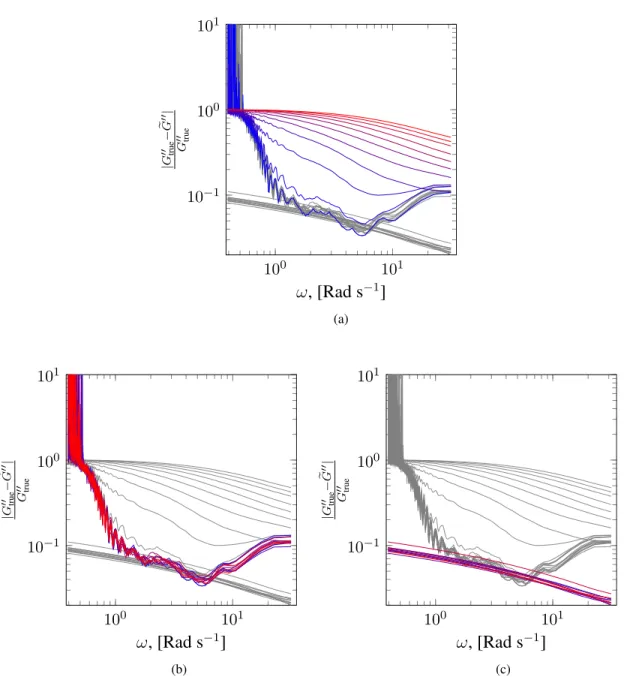
3.3 Impact of linear drift on complex viscosity and dynamic storage and loss moduli for Brownian motion. . . 45
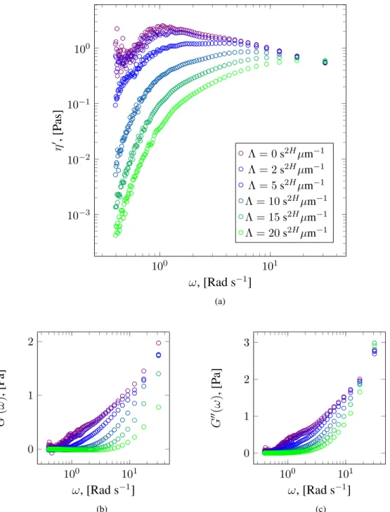
3.4 Impact of linear drift on complex viscosity and dynamic storage and loss moduli for subdiffusive data. . . 46
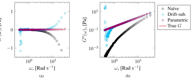
3.5 Dynamic storage,G0, and loss,G00, moduli for simulated Brownian data . . . 52
3.6 Dynamic storage,G0, and loss,G00, moduli for simulated subdiffusive data . . . 52
3.7 Absolute error in the estimation ofG0from the BMdata set . . . 53
3.9 Absolute error in the estimation ofG0from theFBMdata set . . . 55
3.10 Relative error in the estimation ofG00from theFBMdata set . . . 56
3.11 Comparison of Hurst parameter estimation techniques . . . 57
3.12 Comparison of diffusivity estimation techniques . . . 58
3.13 Relative error in estimates ofηgiven by the Stokes-Einstein equation for the BMdata set. . . 58
3.14 Relative error in estimates ofηgiven by the Stokes-Einstein equation for theFBMdata set. . . 59
3.15 Ensemble average estimates of the dynamic storage, G0, and loss,G00, moduli for 1µm diameter particles in 4 wt% HBE mucus. . . 60
3.16 Ratio of the NLS and DLS predictions to the MLE prediction for diffusive parameter values of 1µm diameter particles in 4 wt% mucus. . . 61
4.1 Example of hierarchical clustering. . . 74
4.2 Example clustering applied to the Numerically Generated Heterogeneous Nestonian (NGHN) data set. . . 76
4.3 Test of gap statistic sensitivity . . . 78
4.4 Cluster refinement for the NGHN data set . . . 79
4.5 Final clustering the NGHN data set. . . 80
4.6 Simulated homogeneous Newtonian cluster results . . . 84
4.7 Experimental (sucrose) homogeneous Newtonian cluster results . . . 85
4.8 Simulated homogeneous viscoelastic cluster results . . . 87
4.9 Experimental (HA) homogeneous viscoelastic cluster results . . . 88
4.10 Simulated heterogeneous Newtonian cluster results . . . 91
4.11 Experimental (sucrose) heterogeneous Newtonian cluster results . . . 92
4.12 Simulated heterogeneous viscoelastic cluster results. . . 96
4.13 Experimental (HA) heterogeneous viscoelastic cluster results . . . 97
4.14 Clustering of experimental Agarose data. . . 98
5.1 Approximate scaling of the leading weighting term for the Exact Discrete
approximation to Riemann-Liouville fBm . . . 107 5.2 Ratio of the initial step size for the Exact Discrete approximation to
Riemann-Liouville fBm . . . 109 5.3 Theoretical expected mean FPT from the interval[0,1]starting fromx0=
0.5as a function ofHfor Riemann-Liouville fBm. . . 110 5.4 Scaling of mean FPT from the interval[0,1]with initial locationx0, for
variousH. . . 110 5.5 Time required to achieve a specified bioavailability at the interval boundary
for three values ofH, for three intervals . . . 111
6.1 Overlay of the initial positions of a representative sample of the particle
paths from the AREST CF data set. . . 117 6.2 Example particle path exhibiting no movement over multiple time steps. . . 118 6.3 Initial filtered data points from the AREST CF data set. . . 119 6.4 Example maximum likelihood estimates (MLE) of H and D for two
particles from the AREST CF data set . . . 121 6.5 Representative distribution of the AREST CF data points, grouped based
on their distinguishability from the background fluid. . . 122 6.6 Clustering of pediatric bronchoalveolar lavage samples from the AREST
CF study Background Fluid Points. . . 123 6.7 Clustering of pediatric bronchoalveolar lavage samples from the AREST
CF study without Background Fluid Points.. . . 126 6.8 Maximum likelihood estimates of diffusive parameters with 95%
confi-dence intervals for the AREST CF data set. . . 129 6.9 Comparison of bronchoalveolar lavage sample results from the AREST
CF study to clustering of HBE data. . . 130 6.10 Inter-subject comparison of total cell count inD-Hspace. . . 131 6.11 Patient-level distributions of diffusive parameters from the AREST CF data set. . . 132 6.12 Subject-level predictions of the bioavailability of a 1µm diameter particle
through an airway surface liquid layer . . . 133 6.13 Predicted bioavailability of a 1µm diameter carboxylated particle through
LIST OF ABBREVIATIONS AND SYMBOLS
aBm Amnesic Brownian motion
API Active pharmaceutical ingredient BAL Bronchoalveolar lavage
D Diffusivity
fBm Fractional Brownian motion
FPT First passage time
GSER Generalized Stokes-Einstein relation
H Hurst parameter
HBE Human bronchial epithelial (mucus) iMSD Individual mean squared displacement mBm Multifractional Brownian motion MSD Mean squared displacement
PPTM Passive particle tracking microrheology PC(A) Principal component (analysis)
RL-fBm Riemann-Liouville fractional Brownian motion sBm Standard Brownian motion
CHAPTER 1
Introduction
1.1 Rheology
Fluids are ubiquitous. Their physical properties impact a wide range of processes, from the quotidian (mixing cake batter), to the essential (preventing infections). Rheology is the study of the physical properties of fluids and how those properties respond to applied stress. Newtonian fluids, such as water, exhibit a purely viscous response to stress, dissipating energy, while solids exhibit an elastic response, storing energy. Between these two extremes, there are many synthetic and biological fluids that exhibit properties of both solids and liquids. These are referred to as viscoelastic fluids.
Often, the relative viscous and elastic response to an applied stress is dependent upon the frequency (ω) with which the stress is applied. For purely viscous fluids, the viscosity is the ratio of stress to strain upon deformation, while for viscoelastic fluids, the viscosity is replaced with the complex viscosity,η∗, or the complex shear modulusG∗(s)that divides the frequency dependent stress-to-strain ratio into an in-phase storage component (G0), representing the elastic response, and an out-of-phase, loss component (G00), representing the viscous response. The complex viscosity is directly proportional to the complex shear modulus:iωη∗(ω) =G∗(ω) =G0(ω) +iG00(ω). Fluids may exhibit shear-thickening or shear-thinning depending on which moduli dominates at the relevant frequencies. A mixture of cornstarch and water is a well known fluid that exhibits viscous properties at low frequency forcing and elastic properties at high frequency forcing.
1.1.1 A brief introduction to micro and macrorheology
Rheology may be divided into two main categories. The first, macrorheology, concerns a fluid’s response to an applied stress at the length scales of the fluid volume. A rheometer, consisting of two horizontal plates between which a volume of fluid is placed, is used to apply a controlled stress to the trapped fluid and measure the resulting strain. While protocols for bulk characterization of many fluids have been rigorously established, this approach has three main limitations. First, microliters of the fluid are often required to engender a response above the noise floor of the rheometer while experimental conditions may limit the volume of fluid available for characterization. Second, a rheometer’s noise floor and the fluid’s surface tension, which acts as an elastic force at low driving stress, limits the types of fluids and stress regimes that may be investigated. Third, the physical geometry of the rheometer naturally measures a mean response, spatially averaged over the area of contact between the fluid and the rheometer’s plates. This removes any heterogeneities within the fluid, potentially masking highly discerning information.
Microrheology is an alternative to bulk rheology that is well suited to the characterization of fluids that may be available in limited volumes or exhibit heterogeneity. Furthermore, as we will demonstrate, microrheology may be used to analyze the viscoelastic response of fluids to stresses below the noise floor of most rheometers. Microrheology focuses on the movement of tracer particles embedded in the fluid of interest, informing the linear viscoelastic response of the material across a wide range of frequencies [1–5]. In purely viscous fluids, the viscosity is related to the diffusivity of the embedded tracer particle through the Stokes-Einstein equation,
D= kBT
6πηr, (1.1)
wherekBis the Boltzman’s constant,T is temperature andris the radius of the embedded particle.
and elastic components, provides the foundation for all modern microrheological investigations. In the following section we present Mason and Weitz’s derivation of the GSER.
1.1.2 Generalized Stokes-Einstein Relation
Diffusion refers to the stochastic movement of solute through a fluid and arises from the bombardment of the particles composing the solute by the molecules of the surrounding fluid. The Stokes-Einstein relation (1.1) formally relates the stochastic motion of an individual particle, represented by the diffusivity,D, to the viscosityη of the local fluid. We may think of viscosity as a dampening force, dissipating energy and decreasing the stochastic fluctuations of the particle. Conversely, an increase in the innate energy of the fluid, represented bykBT, serves to increase the
stochastic fluctuations. Following Newton’s second law, the thermal and drag forces acting on a particle must balance, i.e.,
mV˙(t) =Fdrag(t) +Fthermal(t). (1.2) In their generalization of the Stokes-Einstein relation, Mason and Weitz begin with the generalized Langevin equation that presentsFdrag(t)in terms of a damping function with memory kernelζ(t), and Fthermal as a stochastic term representing the random bombardment of the particle with the surrounding molecules [7, 8]:
mV˙(t) =fR(t)−
Z t
0
ζ(t−u)V(u)du. (1.3)
wheremandV are the probe mass and velocity, respectively. Stokes’ law relates the viscosity of the the fluid to the memory kernel,
ζ = 6πηr. (1.4)
LettingL{-}be the standard Laplace transform such that
˜
f(s) =L{f(t)}= Z ∞
0
we may take the Laplace transform of (1.3) and solve for the velocity:
˜
V(s) = mV(0) + ˜fR(s)
ms+ ˜ζ(s) (1.6)
=⇒ V˜(s)V(0) =V(0)mV(0) + ˜fR(s)
ms+ ˜ζ(s) . (1.7)
Taking the ensemble average,h-i, and assuming we are in the zero-mass limit, we find,
hV˜(s)V(0)i= kBT ˜
ζ(s). (1.8)
In practice, the increment process is typically measured, not the velocity process. The time domain mean squared increments,hx2(t)iare directly related to the velocity autocorrelation function through the Laplace transform,
hV˜(s)V(0)i= s
2
2Lhx
2(s)i:= s2
2hx˜
2(t)i. (1.9)
Thus, by substituting into (1.8), the memory kernel may be directly related to the observed increments,
˜
ζ(s) = 2kBT
s2hx˜2(s)i, (1.10)
which is in turn proportional to the complex viscosity of the fluid,
˜
η(s) = ζ(s)˜
6πa. (1.11)
The complex shear modulus may then be related to the mean squared increments of the diffusing particle as,
˜
G(s) =s˜η(s) = kBT
sπahx˜2(s)i. (1.12)
time and subsequently transformed according to (1.12) to estimate the viscous and elastic moduli of the fluid.
Both the generalized (1.12) and non-generalized (1.1) Stokes-Einstein relations are based on two key assumptions. First, the Einstein component relating the thermally activated motion of the probe particle to its mobility requires that the system is in equilibrium, i.e., the particle is not experiencing a net force. This net force may arise from convective flow within the fluid volume, active manipulation of the particle, either by internal or external forces, or induced by technical deficiencies such as drift of the microscope stage [6, 9, 10]. Second, the Stokes component of (1.12) and (1.1) require that the fluid under investigation is homogeneous, isotropic and incompressible. The homogeneity requirement is often invalidated in gels and synthetic polymer solutions [11–15], as well as various biofluids [16–19], however Squires and Mason [6] point out in their excellent review that the conditions under which the Stokes component fails are themselves important indicators of a material’s properties and are worth investigating. Importantly, heterogeneity may arise from three distinct sources, temporal changes in the fluid or probe particle, spatial variations in fluid constituents and length-scale dependent structural variations within the fluid. Incongruities in any of these variable, time, location, or length-scale, have the potential to engender disparate estimations of a heterogeneous fluid’s viscoelastic properties.
1.2 Motivations and objectives
particularly micron-scale drug delivery particles and dry powder formulations that are large enough to interact with the elastic network of mucin proteins that make up mucus, and endow it with its viscoelastic properties.
The impact of the mucosal layer on the distribution of micron-scale drug delivery particles and dry powder formulations is a complex function of the compound’s surface chemistry and size, as well as the physical properties of the mucosal layer itself. The mucosal layer dictates the movement of these compounds as they dissolve or decompose, significantly influencing the concentration time profile of the embedded active pharmaceutical ingredients (API). It is increasingly recognized that the diffusive properties of microscopic particles in viscoelastic fluids are not only anomalous, and poorly described by Brownian motion [23–28], thus invalidating a central assumption of most pharmacokinetic models, but they exhibit potentially biologically relevant inter-patient variability due to age, genetics, disease progression and environmental conditions [22, 23, 29, 30]. The design of therapeutics for controlled delivery of an API through the mucosal layer requires statistical and mathematical tools to analyze experimental data, perform model selection, fit model parameters, and forecast outcomes. No current methodology adequately address the unique and highly variability properties of the mucosal layer that can significantly influence diffusion, API uptake and subsequent bioavailability of therapeutic compounds. Here, we seek to provide a first step toward such a methodology.
The application of this research to pulmonary drug delivery is of particular interest because pulmonary drug delivery has been shown to lead to a reduction in side effects and faster drug onset times [31, 32]. Pulmonary drug delivery has been identified as a potentially superior method of drug delivery for a range of conditions such as chronic obstructive pulmonary disease, asthma and cystic fibrosis. Inhalation has also been proposed as a delivery route for vaccines, gene therapies, insulin treatments and cancer treatments [31]. The rigorous analysis of the diffusive movements ofspecifictherapeutic compounds through the pulmonary mucosal layer ofspecificpatients will facilitate personalized medical treatments for a wide range of conditions. The ability to perform these evaluations transiently holds great promise to couple patient characteristics and drug treatments, and to modify treatments in real time.
and how those properties change depending upon the characteristics of the therapeutic compound. The GSER significantly advanced the field of microrheology beyond its initial applications and the seminal work of Mason and Weitz has been been adapted to the study of a wide variety of viscoelastic fluids across a range scientific disciplines [33–36]. However, as microrheology techniques are applied to increasingly complex fluids such as mucus, two hurdles must be addressed: the differentiation of thermally-activated motion from driven motion in the probe particle’s trajectory, and the presence of spatial or temporal heterogeneity due to changes in the local physical properties of the fluid, or changes in the surface chemistry or physical size of the particle itself. Furthermore, to make the this methodology practical, more accurate models for particle diffusion must be developed, and a theoretical framework is required to predict particle passage times, and subsequent bioavailability, beyond experimentally-observable time scales.
1.3 Overview
In the remaining chapters, we propose best practices addressing the hurdles outlined above. Chapter 2 presents existing Brownian models for the diffusive movements of particles in homoge-neous and heterogehomoge-neous, viscous and viscoelastic fluids, with a focus on simulation algorithms for each model. We conclude with a novel model based on fractional Brownian motion for diffusion in heterogeneous viscoelastic fluids and demonstrate how its simulation algorithm may be adapted to address the inverse problem of parameter estimation given a single realization of such a stochastic process.
In Chapter 3 we discuss approaches to diffusive parameter estimation when driven motion is coupled to a particle’s thermally-activated movements. We demonstrate the impact of driven motion on traditional parameter estimation techniques, as well as the recovery of the storage and loss moduli, and viscosity of the fluid.
the proposed algorithm is able to accurately and consistently quantify heterogeneity in complex fluids.
No explicit formula currently exists for the first passage time of a fractional Brownian process from the unit interval. In Chapter 5 we motivate a functional form for this quantity through analysis of the simulation algorithms discussed in Chapter 2. This analysis highlights an initially unintuitive feature of fractional Brownian motion–that subdiffusive processes travel faster over short distances than superdiffusive processes. These results emphasize the importance of accurately estimating diffusive parameter values and quantifying the spacial dimensions over which diffusion occurs.
CHAPTER 2
Brownian Diffusion Models and Simulation Algorithms
In this chapter we discuss several models for the diffusive movements of nano- and micro-scale particles. We begin with Brownian motion, a well-known model appropriate for homogeneous, purely viscous fluids, and progress toward models suitable for diffusion in heterogeneous, viscoelastic fluids. Simulation techniques for each model are detailed.
2.1 Introduction
Following its formal mathematical description by Einstein in 1905 [37], Brownian motion has become a foundational model, linking the mobility exhibited by a particle to the physical properties of the surrounding fluid via the Stokes-Einstein relation (1.1). However, similar to the breakdown of the Stokes-Einstein relation in the presence of both viscous and elastic components, requiring the GSER (1.12), a generalization of Brownian motion, or an alternative model, is required to adequately describe the movement of particles in viscoelastic fluids. To this end, several Brownian processes have been proposed to address diffusion in viscoelastic, and heterogeneous viscoelastic fluids. Developing appropriate descriptions for the diffusive movement of particles is essential for the accurate forecasting of desired statistics such as, in the context of transmucosal drug delivery, the concentration time profile of an inhaled formulation at the mucus-epithelial interface, or the time course of systemic exposure. The absence of closed-form diffusive transport equations applicable to heterogeneous viscoelastic fluids requires the development of efficient methods to generate diffusive trajectories of individual particles and the pursuit of the desired statistics through rigorous simulations.
subcategories, Weyl (Section 2.3) and Riemann-Liouville (Section 2.4) based on the definitions of their respective fractional derivatives. In viscoelastic fluids, the elastic modulus introduces memory, i.e., correlation, in the probe particle’s increment process. For fBm processes of both types, this memory is characterized by a unitless constant known as the Hurst parameter,H ∈ [0,1]where H >0.5andH <0.5correspond to positive correlation (superdiffusion) and negative correlation (subdiffusion) in the particle’s increments. WhenH = 0.5, the increments are uncorrelated and sBm dynamics are recovered. mBm is the generalization of fBm for time-varyingHcaused by the movement of the probe particle between regions of a fluid with different elastic moduli (Section 2.5). In this chapter, we present strengths, weaknesses and simulation techniques for each model. We con-clude by introducing amnesiac Brownian motion, an alternative model for diffusion in heterogeneous viscoelastic fluids (Section 2.6).
2.2 Standard Brownian motion
sBm, the most common Brownian model, was first formulated by Einstein based on his observa-tions of pollen particles in water [37]. While sBm is a ubiquitous model for diffusion, it is best suited for “ideal” diffusion through homogeneous, purely viscous, i.e., non-viscoelastic, fluids. A sBm process, denoted{S(t)}, is a Gaussian process with stationary increments. The following properties also hold:
(i) S(0) = 0 (ii) E[S(t)] = 0 (iii) E[S2(t)]∼t
A continuous-time sBm process may be written as
S(t) = Z t
0
ξ(u)du, (2.1)
are Gaussian and uncorrelated. sBm may be easily simulated by computing the cumulative sum of normally distributed iid numbers. A particle position process with inter-observational time∆tis
Xn=X(n∆t) = n
X
i=0
ξi, ξ ∼ N(0,∆t), (2.2)
whereN(0,∆t)is the normal distribution with mean zero and variance∆t.
Because the increments are uncorrelated, sBm is not well suited for modeling subdiffusive processes that exhibit correlation in the increment process. A common scenario engendering subdiffusion is the passive, thermally activated movement of particles in viscoelastic fluids where the elasticity of the fluid’s gel-structure introduces correlation in the particle’s movement. To model such phenomena for which sBm is poorly suited, we turn to fBm.
2.3 Weyl fractional Brownian motion
2.3.1 Theory
Weyl fractional Brownian motion (W-fBm) is a generalization of sBm based on the Weyl fractional integral and allows for correlation in the increment process. W-fBm was first formulated by Kolmogorov in 1940 [38] and later popularized by Mandelbrot and Van Ness [39]. A W-fBm continuous time position process{B(t)}may be write as,
BH(t) = 1
Γ(H+1/2)
Z 0
−∞ n
(t−u)H−1/2
−(−u)H−1/2o
ξ(u)du+ Z t
0
(t−u)H−1/2 ξ(u)du
. (2.3) Similar to sBm, W-fBm is a Gaussian process and exhibits the following properties:
(i) BH(0) = 0
(ii) E[BH(t)] = 0
(iii) E[B2
H(t)]∼t2H
whereHis the Hurst Parameter. As noted earlier, W-fBm processes may exhibit negative correlation (H < 0.5), giving rise to sub-diffusion, or positive correlation (H > 0.5), giving rise to super-diffusion, i.e., persistent motion, and whenH = 0.5the increment process is uncorrelated and standard Brownian dynamics are recovered. From (2.3) we see that W-fBm may be thought of as an infinite history, represented by the integral from−∞to 0, combined with a finite moving average, represented by the integral from 0 tot. While the increment process resulting from only the later integral is non-stationary, the summation of both integrals leads to stationarity of the increments [40].
The correlation in the position process for W-fBm is given by
ACFB(t1, t2) =E[BH(t1)BH(t2)] =
1 2 t
2H
1 +t22H− |t2−t1|2H (2.4)
and autocorrelation of the discrete incrementsbn=Bn+1−Bnis
ACFb(n) =cov(bk, bk+n) =
1 2σ
2∆t2H |n+ 1|2H +|n−1|2H −2|n|2H (2.5)
where the subscriptHhas been dropped for clarity.
W-fBm has been used to model processes as diverse as river flow [41–44] and network traffic [45, 46]. In a biological setting, it has been used to describe the movements of 1µm diameter particles in human bronchial epithelial mucus [23] and intra-cellular biopolymers [47], among other applications. For particle diffusion, the following stochastic model for the particle’s position processX(t)has been proposed [25]:
X(t) =µt+σBH(t). (2.6)
Here,BH(t)is a zero-mean Gaussian process specified by (2.3) andσis a scaling factor that may be
2.3.2 Simulation techniques
2.3.2.1 Direct algorithm
Direct algorithms for W-fBm generate sample paths by multiply a decomposition of the cor-relation matrix specified by (2.4) with vectors of normally distributed random numbers [48, 49]. This approach may be implemented using the square root decomposition of the correlation matrix, however it is more computationally efficient to consider the Cholesky decomposition. To generate a position process of lengthN, we first build the correlation matrixΛ. Entryi, jofΛis
Λi,j =
1 2 t
2H
i +t2jH − |ti−tj|2H, (2.7)
fori, j= 1, ..., N. LetLbe the lower triangular matrix resulting from the Cholesky decomposition
ofΛsuch thatLL0 =Λ. The position process of a particle diffusing via W-fBm is then generated as
X =σ1/2(Lξ), whereξ iid∼ N(0,∆t)is aN ×1vector. The matrixLserves to weight the white noise terms in order to produce a processXtwith the desired correlation structure. In general we
have,
Xj =σ
1/2
[ξ1L1,j+ξ2L2,j+...+ξjLj,j]. (2.8)
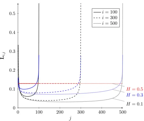
Figure 2.1 shows the Cholesky weights of paths of lengthN = 500for three values ofHat various points in the path.
The Direct W-fBm simulation algorithm is straight forward, however, in its current presentation, the length of the path must be specified a priori. This makes the algorithm poorly suited for adaptive implementations where the simulated path is extended until a stopping condition is met. Furthermore, Cholesky decomposition is computationally expensive since most algorithms exhibit
O(N3)complexity [50].
2.3.2.2 Frugal Cholesky updates
0 100 200 300 400 500 0 0.1 0.2 0.3 0.4 0.5
H= 0.1 H= 0.3
H= 0.5
j
Li,j
i= 100 i= 300 i= 500
Figure 2.1: Cholesky weights of threeN = 500step paths(∆t = 1/60) based on the Weyl-fBm
covariance (2.7). The Hurst parameter of the paths areH = 0.1 (black), H = 0.3 (blue) and H = 0.5(red).Thei≤jweightsLi,jused to constructXj are shown for three points in the path,
j= 100,j= 300andj= 500. For the Brownian path (H= 0.5), all weights are equivalent.
givenΛ∈RN×N only requires the computation of one additional row. Le, the resulting Cholesky decomposition ofΛe, is a lower triangular matrix of size(N + 1)×(N+ 1)such thatLeLe0 = Λe.
Similar to the relationship betweenΛandΛe,LeandLdiffer only in their last row, i.e.Lei,j =Li,j for
i, j= 1,2, ...N. Therefore, calculatingLe, the new Cholesky matrix, based onL, the old Cholesky
matrix, andΛe, the correlation matrix at the current time step, isO(N)times more efficient than directly computing the full Cholesky decomposition ofΛe. The elements in theNthrow ofLe are
given by
e
LN,j =
1 e
Lj,j
" e
ΛN,j − j−1
X
k=1
e
LN,kLej,k
#
, (2.9)
e
LN,N =
" e
ΛN,N −
NX−1 k=1
e
L2N,k
#1/2
Importantly, the Direct algorithm has the property that rowj−1ofLis not a subset of rowjof
L, therefore at each stage of the algorithm,jnew weights must be explicitly calculated leading to
O(N2)complexity.
2.3.2.3 Hypergeometric Discrete algorithm
Discrete algorithms are based on discrete approximations to the continuous time position process (2.3). They have the form,
XN = N
X
i=1
Z i∆t
(i−1)∆t
f(u, t, H)ξidu, (2.11)
where the weighting function f(u, t, H) depends on the version of the algorithm. The general approach is to find a set of weights that produce W-fBm when multiplied by the noise termsξi. The
primary benefit of Discrete algorithms compared to Direct algorithms is that they are well suited for adaptive simulation schemes since the weights forXN are a subset of the weights forXN−1 and
new positions can be appended to the existing position process simply by evaluating the appropriate weight function.
The hypergeometric Discrete algorithm is based on an alternative representation of the continuous time W-fBm process described by (2.3). It is written as [51]:
BH(t) =
Z t
0
KH(t, u)ξ(u)du (2.12)
where
KH(t, u) = (t−u)
H−1/2 Γ(H+1/2) ×2F1
H−1
2, 1
2−H;H+ 1 2; 1−
t u
, t > u. (2.13)
As an aside, the above equation is presented as it is in Carmona et al. [52] who cite the work of Decreusefond [51]. Decreusefond however, defines the Gaussian hypergeometric function as
F
2 1(a, b;c;z), |z|<1. (2.14)
The condition onzis clearly not satisfied in the presentation given by Carmona et al. ift > u. F
F
2 1(a, b;c;d) =
∞ X
n=0
(a, n)(b, n) (c, n)
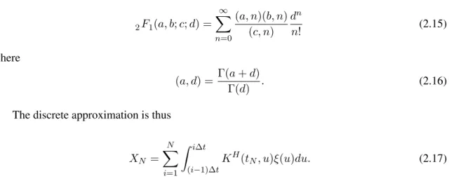
dn
n! (2.15)
where
(a, d) = Γ(a+d)
Γ(d) . (2.16)
The discrete approximation is thus
XN = N
X
i=1
Z i∆t
(i−1)∆t
KH(tN, u)ξ(u)du. (2.17)
Exact calculation of the above integral is inefficient to compute, but for sufficiently small∆t, the integral may be approximated with techniques such as the Mid Point method, the Trapezoidal method or Gaussian quadrature. For the simulations presented here, we utilize the Trapezoidal method.
0 600 1,200 1,800
10−1.4
10−1.2 10−1 10−0.8
10−0.6 10−0.4
H = 0.2 H = 0.3
H = 0.4
j wj
Direct Discrete Hyp.
The weights for the Direct and Hypergeometric Discrete W-fBm algorithms are presented in Fig. 2.2. We make two observations: First, the Direct weights for points early in the time series are larger than the weights for points in the middle of the time series and thus have a larger influence onXN.
Second, the Hypergeometric Discrete approximation does not capture this trend. The pronounced influence of the initial noise terms for W-fBm processes is intimately linked to the representation of W-fBm as an infinite memory process. In simulating such processes, it is assumed that the first data point incorporates the infinite “pre-history”. This initial pre-history, whatever it may be, is then perpetuated throughout the length of the simulated path via the large weights assigned to the initial noise components. While this may seem like a reasonable approach in theory, many physical phenomena, such as diffusion processes, have a well defined commencement at somet = 0, at which point there is no memory in the process. W-fBm as a model for diffusion incorporates infinite memory att= 0that we do not expect to exist in the physical phenomena itself. We will refer to this as the Starting Point Problem. As noted by others [40, 53–55], this fundamental difference between the model and the physical phenomena it is tasked with describing, calls into question the use of W-fBm in this context. To address this miss-match caused by the Starting Point Problem, we turn to Riemann-Liouville fractional Brownian motion.
2.4 Riemann-Liouville fractional Brownian motion
2.4.1 Theory
Riemann-Liouville fractional Brownian motion (RL-fBm), is a an alternative representation of fBm based on the Riemann-Liouville fractional integral [56]. A RL-fBm continuous time position process{B(t)}may be written as,
BH(t) = 1
Γ(H+1/2)
Z t
0
(t−u)H−1/2
Correlation of the RL-fBm position process [54] is given by
E[BH(t1)BH(t2)] =
tH+1/2
1 t
H−1/2
2
(H+1/2)[Γ(H+1/2)]2 ×2F1
1
2 −H,1, H+ 3 2, t1 t2 , (2.19)
where0< t1 < t2and2F1is the Gaussian hypergeometric function defined in (2.15).
To get the variance of the RL-fBm position process, we sett1 =t2, thus
E[BH2(t)] = 2t
2H
(H+1/2)[Γ(H+1/2)]2 ×2F1
1
2 −H,1, H+ 3 2,1
(2.20)
= 2t
2H
(H+1/2)[Γ(H+1/2)]2
Γ(H+3/2)Γ(2H)
Γ(2H+ 1)Γ(H+1/2)
(2.21)
= t
2H
H[Γ(H+1/2)]2, (2.22)
and we recognize that the variance scales witht2H as expected.
Given a RL-fBm process with total path lengthtand inter-observational time∆tsuch that we may assume the increments are locally asymptotically stationary, their correlation is given by [40]
ACFb(n) =
σ2+{2H(Γ(H+1/2)}2−1
(n∆t)2H (2.23) whereσ2 =hB2
H(1)i.
2.4.2 Simulation techniques
2.4.2.1 Direct algorithm
We can easily implement a Direct algorithm for the simulation of RL-fBm using the same method described in Section 2.3.2.1 for W-fBm. Whereas for W-fBm the covariance matrix was defined by (2.4), here we simply substitute (2.19) to form a covariance matrix for RL-fBm, denoted
Φ. Thei, jelement ofΦis
Φi,j =
tH+1/2
i t
H−1/2
j
(H+1/2)[Γ(H+1/2)]2 ×2F1
1
2 −H,1, H+ 3 2,
tj
ti
2.4.2.2 Exact Discrete algorithm
The Exact Discrete RL-fBm algorithm is based on the discrete position process [57]
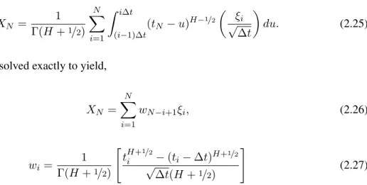
XN =
1 Γ(H+1/2)
N
X
i=1
Z i∆t
(i−1)∆t
(tN −u)H−
1/2 ξi √ ∆t du. (2.25)
The integral can be solved exactly to yield,
XN = N
X
i=1
wN−i+1ξi, (2.26)
wi =
1 Γ(H+1/2)
" tH+1/2
i −(ti−∆t)H+1/2 √
∆t(H+1/2)
#
(2.27)
Figure 2.3 shows the weightswN−i+1 for three paths with three different Hurst parameters.
0 100 200 300 400 500
0 0.1 0.2 0.3 0.4 0.5 0.6 0.7
H = 0.1
H = 0.3
H = 0.5
j wi,j
i= 100 i= 300 i= 500
Figure 2.3: Weights for threeN = 500step paths (∆t = 1/2) generated via the Exact Discrete
RL-fBm algorithm. The paths have Hurst parameterH= 0.1(black),H= 0.3(blue) andH= 0.5 (red). The weights used to construct XN are shown for three points within each path, j = 100,
2.4.2.3 Improved Discrete algorithm
Rambaldi et al. [57] and Muniandy et al. [54] utilize an improved weighting method that exactly satisfies the local scaling behavior of the covariance. Specifically,
XN = N
X
i=1
ξiweN−i+1 (2.28)
where,
e wi =
1 Γ(H+1/2)
t2iH −(ti−∆t)2H
2H∆t
1/2
. (2.29)
1 2 3 4 5
2 2.5 j W eight wj e wj (a)
1 2 3 4 5
−0.2 0 0.2 tj X ( tj ) (b)
Figure 2.4: Comparison of weights for the Improved and Exact Discrete RL-fBm algorithms. (A) The newest Brownian noise component,ξN receives a higher weight for the Improved algorithm
compared to the Exact algorithm. (B) The impact of the increased weight for trailing Brownian noise components in the Improved algorithmm is that the position process of the resulting path is slightly more extreme compared to the Discrete algorithm.
A comparison of the Exact and Improved weights over the length of a short path (N = 5) is shown in Fig. 2.4. The newest Brownian noise component,ξN, receives a higher weight for the
Improved algorithm compared to the Exact algorithm. The two weighting functions are monotonic and convergent for earlier time points, i.e., asN−i+ 1increases. The increased weight onξN in
W-fBm algorithms. Within RL-fBm algorithms, the Discrete approaches have the advantage that they are straightforward to compute and do not require the evaluation of the Gaussian hypergeometric function, which is unwieldy, requiring different algorithms for different parameter values.
0 600 1,200 1,800 10−1.4
10−1.2 10−1 10−0.8 10−0.6 10−0.4
H= 0.2 H= 0.3
H= 0.4
j wj
Direct Exact Disc. Improved Disc.
Figure 2.5: Comparison of weights for the Direct, Exact Discrete and Improved Discrete RL-fBm algorithms forH = 0.2(black),H = 0.3(blue) andH = 0.4(red). The weights are for a path of temporal lengthT = 30s, inter-observational time∆t=1/60andN = 1,800steps. The difference
0 200 400 600 800 1,000 1,200 1,400 1,600
−5
−4
−3
−2
−1 0 1 2 3
tj
X
(
tj
)
Direct, W-fBm Direct, RL-fBm Hyp. Disc., W-fBm Exact Disc., RL-fBm Imp. Disc., RL-fBm
Figure 2.6: Comparison of position processes from W-fBm and RL-fBm algorithms. The paths have a temporal lengthT = 30s with inter-observational time∆t=1/60andN = 1,800steps. The gray
400 405 410 415 420 425 430 435 440 445 450
−2
−1.8
−1.6
−1.4
−1.2
−1
−0.8
−0.6
−0.4
−0.2
tj
X
(
tj
)
Direct, W-fBm Direct, RL-fBm Hyp. Disc., W-fBm Exact Disc., RL-fBm Imp. Disc., RL-fBm
Figure 2.7: Comparison of position processes from W-fBm and RL-fBm algorithms. The paths have a temporal lengthT = 30s with inter-observational time∆t=1/60andN = 1,800steps. The data
2.5 Multi-fractional Brownian motion
2.5.1 Theory
Multi-fractional Brownian motion (mBm) is a generalization of fractional Brownian motion that allows for a time-varying Hurst parameter [58, 59]. Here, we focus on Riemann-Liouville mBm although various representations of mBm exist [60, 61]. The continuous time (RL) mBm process is defined as [55]
BH(t)(t) = 1 Γ(H(t) +1/2)
Z t
0
(t−u)H(t)−1/2
ξ(u)du, t≥0, (2.30)
and has covariance,
ACFB(t1, t2) =
2tH(t1)+1/2
1 t
H(t2)−1/2
2
[2H(t1) + 1] Γ(H(t1) +1/2)Γ(H(t2) +1/2)×2F1
1
2 −H(t2),1, H(t1) + 3 2,
t1
t2
, (2.31) wheret2 > t1. We observe that the key difference between mBm and RL-fBm is the substitution of
the functionH(t)for the constantH.
2.5.2 Simulation techniques
Muniandy et al. [55] propose Exact and Improved Discrete algorithms for mBm using the same weighting functions described by (2.29) and (2.27), without modification. Their approach is as straight forward as it is computationally expensive. The position process is simulated as
Xj =BH(tj)(tj), 0≤j≤N. (2.32)
Forkdiscrete values ofH, we recognize that (2.32) calls for the simulation ofkdistinct RL-fBm processes, whose elements are then selectively recombined according toH(tj). For example, given
H(tj), we use the appropriate RL-fBm Discrete algorithm to generateBH(ti)(ti),0 ≤i≤j, and
store the final positionB(tj)asX(tj). At the next time step, ifH(tj+1) 6= H(tj) we generate
H(tj+1) =H(tj), we simply extend the current path by one step and store the result in the same
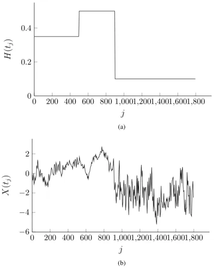
manner. Let
H(tj) =
0.35 0≤j≤500 0.5 500≤j≤900 0.1 900≤j≤1800
(2.33)
Figure 2.8 shows the position process resulting from this choice ofH(t).
0 200 400 600 800 1,0001,2001,4001,6001,800 0 0.2 0.4 j H ( tj ) (a)
0 200 400 600 800 1,0001,2001,4001,6001,800
−6 −4 −2 0 2 j X ( tj ) (b)
Figure 2.8: Example mBm path simulated using Discrete Improved weights. The paths have a temporal lengthT = 30s with inter-observational time∆t=1/60andN = 1,800steps. (A) The
input functionH(tj)is defined by (2.33). (B) The resulting possition process givenH(tj).
However, mBm is not without limitations. To understand these, consider a biphasic fluid, the left volume of which is a purely viscous fluid and the right volume of which is a viscoelastic fluid.Within each region, the fluid is homogeneous. Consider a particle that has been deposited in the purely viscous half of the volume at timet= 0. While the particle diffuses within the viscous fluid, we would apply standard Brownian motion to model its movements since there would be no correlation in the increment process. As soon as the particle transits to the viscoelastic half of the volume, we would instinctively apply RL-fBm to account for the correlation in the increment process created by the non-zero storage modulus of the fluid in that region. Within the viscoelastic region, we note that the diffusive movements of the embedded particle does not meet the formal definition of a long memory process. The formal definition of a long memory process is a process such that
ACF(t)∼ct2d−1 ast→ ∞, (2.34)
wherec6= 0andd <0.5[62]. In the case of RL-fBm (and W-fBm), the covariance scales asct2H, andH ∈ [0,0.5] =⇒ d∈ [0.5,1], thus, formally, there is no long-time memory. The weights however,do decayasct2d−1withd <1/2. To see this, consider the formula for the Exact Discrete
weights given in (2.27). Ignoring the leading gamma term, we have,
wi ={ √
∆t(H+1/2)}−1/2htH+1/2
i −(ti−∆t)H+
1/2i
(2.35)
={√∆t(H+1/2)}−1/2
tiH+1/2−tiH+1/2−∆t(H+1/2)tH−1/2
i +
1 2∆t
2(H−1/
2)(H+1/2)tiH−3/2+O(∆t3)
(2.36) = ∆t1/2tH−1/2+1
2∆t 3/2(H
−1/2)tH−3/2+
O(∆t5/2) (2.37)
Asti → ∞, the first two terms satisfy the scaling relation in (2.34) when H < 1/2. Thus, even
though RL-fBm is not formally a long memory process, we would be remiss to neglect any of the noise terms in the calculation ofXN, even wheniN.
particle in the viscoelastic fluid is dependent upon its previous behavior in the purely viscous fluid. Furthermore, under the mBm model, the movement of the particle in the viscoelastic half of the fluid volume would depend on the stochastic movements of the particle in the purely viscous halfas if the purely viscous half had been viscoelastic.We know this is inconceivable since there is no physical mechanism in the viscous fluid to store and transmit the particle’s movements to the viscoelastic region for perpetuity, or otherwise. We refer to this as the “Agency Problem.” This phenomena is manifested in mBm through the use ofH(t)as the exponent of the integrand in (2.30) and gives rise to discontinuity in the position processX(t)whenH(t)is not a smooth function, and for many fluids, we have no reason to suspect this to be true. To address the Agency Problem, we introduce amnesiac Brownian motion.
2.6 Amnesiac Brownian motion
2.6.1 Theory
Continuous time amnesiac Brownian motion (aBm), presented here for the first time, is gener-alization of RL-fBmn which addresses the Agency Problem. It may be used to simulate processes with both constant and variable Hurst parameter, i.e., diffusion in heterogeneous and homogeneous, viscous and viscoelastic fluids. An aBm position process may be written as
BH(t)(t) =
1 Γ(Ht(t) +1/2)
Z t
0
(t−u)Ht(u)−1/2
ξ(u)du, t≥0 (2.38) The key difference between aBm and mBm is the use ofH(u)in the integrand, as opposed toH(t).
To develop an intuitive understanding of aBm consider a volume of fluid with four regions, each region containing a different fluid with an storage modulus characterized by the appropriate corresponding Hurst parameter. From left to right, the respective values ofHfor each region are, H = 0.4,H = 0.5,H = 0.1andH = 0.2. A particle, initially in the first region, is allowed to diffuse through the fluid and six observations of its location are made. This scenario is illustrated in Fig. 2.9.
For an mBm process, we would write the positionYn=Y(n∆t)as
Y2 =ξ1w1,H=0.4+ξ2w2,H=0.4 (2.40)
Y3 =ξ1w1,H=0.5+ξ2w2,H=0.5+ξ2w3,H=0.5. (2.41)
Note that the weightsware a function ofHat the particle’s current position. Under an aBm model, we may similarly write the first three positions as
X1 =ξ1w1,H=0.4 (2.42)
X2 =ξ1w1,H=0.4+ξ2w2,H=0.4 (2.43)
X3 =ξ1w1,H=0.4+ξ2w2,H=0.4+ξ2w3,H=0.5. (2.44)
Up to this point, the aBm and mBm processes for this scenario differ only by the third position. At this point, for the mBm process,Y3is generated as if the particle had only inhabited theH = 0.5
region, as evidenced by the use of the weightsw,H=0.5. According to the formulation of mBm (2.32)
the fourth position should be written as
Y4 =ξ1w1,H=0.1+ξ2w2,H=0.1+ξ3w3,H=0.1+ξ4w4,H=0.1. (2.45)
Here, an even more extreme change in behavior has happened, the fourth position is calculated assuming that all previous behavior had happened in theH = 0.1region. In contrast to mBm, the fourth position, under an aBm model, is simply
X4 =ξ1w1,H=0.5+ξ2w2,H=0.5+ξ3w3,H=0.5+ξ4w4,H=0.1. (2.46)
The remaining aBm positions are,
X5 =ξ1w1,H=0.5+ξ2w2,H=0.5+ξ3w3,H=0.5+ξ4w4,H=0.2+ξ5w5,H=0.2 (2.47)
X6 =ξ1w1,H=0.5+ξ2w2,H=0.5+ξ3w3,H=0.5+ξ4w4,H=0.2+ξ5w5,H=0.2+ξ6w6,H=0.1. (2.48)
H = 0.4 H = 0.5 H = 0.1 H = 0.2
X1
X2 X
3
X4 X5
X6
Figure 2.9: Illistration of diffusion through a spatially heterogeneous fluid. A particle, beginning in the first region, is allowed to diffuse through the volume of fluid. Each region exhibits a different level of memory characterized by their respective Hurst parameters.
1 2 3 4 5 6
−1.2
−1
−0.8
−0.6
−0.4
−0.2 0 0.2 0.4
j Xj
aBm mBm
Figure 2.10: Example aBm and mBm paths corresponding toH(tj)presented in Fig. 2.9. Both
2.6.2 Simulation Techniques
2.6.2.1 Path Splicing
The path splicing algorithm relies on the assumption that, in nature, the bombardment of the diffusing particle by the molecules of the surrounding fluid, represented here by the noise termξ, cannot impact the position of the particle for an infinite amount of time, i.e., we assume there exists a ψsuch that
Pψ i=1wi
PN i=ψ+1wi
≈0. (2.49)
This allows us to write the current state of an aBm process as a function of a finite number of previous states. Adjacent segments can then be “spliced” together by incorporating the noise terms used in the finalψsteps of the previous path segment into the initialψsteps of the next path segment. To construct a position process of lengthN made of segments of lengtha > ψ, we need only compute thea×acorrelation matrix. The first segment is given by,
{X}1 =σ1/2
ξ1
1 ξ21 · · · ξa1
VH(t1), (2.50)
whereVH(t1)is thea×aweight matrix of the first segment andξ∼ N(0,1). The elements of the weight matrix may be specified using any of the RL-fBm methods previously discussed. Here we use the Discrete Improved weights defined in (2.29). The superscripts on theξterms indicate that they are associated with the first segment. Each subsequent segmentb6= 1is constructed as follows,
{X}b =σ1/2
ξab−−1q+1 ξab−−1q+2 · · · ξb−1
a ξqb+1 ξqb+2 · · · ξba
VH, (2.51)
whereq≥ψis a measure of the overlap between adjacent segments. Note that for uniformH, the correlation matrix for each segment is the same, thus we only need to computeVonce. To use this
algorithm to simulate diffusion through heterogeneous media, we simply keep track of the Hurst parameter along the length of the segment and use this record to build the appropriate correlation matrix. At each time step whereH(tj)6=H(tj−1), only theaweights in the final row ofVH(tj)
need to be calculated.
g
{X}b ={Xqb+1· · ·Xab}+ζ (2.52) and
ζ =Xab−1−Xqb. (2.53)
The shift of segmentbbyζensures that the paths are continuous.
2.6.2.2 Modified Discrete Algorithms
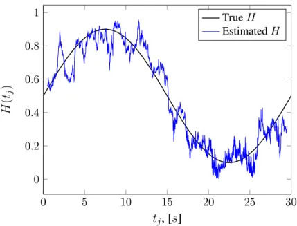
Both the Improved Discrete and Exact Discrete algorithms may be modified to efficiently generate aBm process without resorting to path splicing if the assumption that the impact of noise increments exhibit a finite duration does not hold. To do so, we only need to keep track of the values ofHassociated with each previously time step. Figure 2.11 shows an example aBm path generated using a modified Improved Discrete algorithm where
H(tj) = 0.4 sin
j2π
N
+ 0.5. (2.54)
0 5 10 15 20 25 30 0
2·10−2 4·10−2
6·10−2
8·10−2
0.1
tj, [s]
Xj
,[
µ
m]
Figure 2.11: Example aBm path with sinosodialH specified by (2.54). The path was generated using a modified Improved Discrete algorithm and hasN = 1,800steps and inter-observational time ∆t=1/60s, andD= 0.005µm2s−2H.
2.7 Local estimations ofH
There are many alternative approaches to simulating exact and approximate fBm processes, such as the spectral, wavelet-based and Random Midpoint Displacement methods (for an excellent review, see [63, 64]). However, in this chapter, we have focused on a subset of methods that involve multiplication of a weight matrix by a vector of noise increments because they naturally give rise to efficient methods for local estimation ofHandD.
LetBH(t)be fractional Gaussian noise with Hurst parameterHdefined. The position process
of a particle undergoing diffusion may be modeled as
X(t) =σBH(t), (2.55)
with inter-observational time∆t,Xn:=X(n∆t)andxn:=Xn=1−Xn,n= 1,2, ...N+ 1. The
distributed and the corresponding log-likelihood function, givenxandHis
`(σ|x, H) =−1
2 (
x0VH−1x
σ2 +Nlog(σ
2) + log(|V H|)
)
, (2.56)
whereVH is the correlation matrix of the increment process. The derivative of (2.56) with respect to
σis
d
dσ`(σ|x, H) =− 1 2
(
−2x0VH−1x σ3 +
2N σ
)
(2.57)
= x 0V−1
H x
σ3 −
N
σ (2.58)
Setting (2.57) equal to zero and solving forσ2, we get
b σ2 = x
0V−1 H x
N (2.59)
Given this maximum likelihood estimationsσ, the probability of observing the data isp(x, H|σ) = `(σ|x, H). Substitutingbσinto (2.56), we see
p(x, H|bσ) =`(σb|x, H) =−1
2 (
x0VH−1x b
σ2 +Nlog(bσ
2) + log(|V H|)
)
(2.60)
=−1
2 (
N x0VH−1x x0V−1
H x
+Nlog(bσ2) + log(|VH|)
)
(2.61)
=−N 2
1 + log(σb2) + 1
N log(|VH|)
(2.62)
We have the Cholesky decompositionLofVH such thatLL0 =VH. We also know that
|VH|=|L|2=
hY Li,i
i2
(2.63)
If we assume thatHis constant, thenL1,1=Li,i∀i= 2,3, ...N when using the Improved Discrete
or Exact Discrete weighting scheme. Therefore
=⇒ 1
N log(|VH|) = 2N
N log(L1,1) = 2 log(L1,1). (2.65) A local estimation ofHandDcan be computed by maximizing (2.60) for a subset of the path. Here, we have implemented a simple local estimator ofHfor overlapping neighborhoods ofn= 60 steps in width. The algorithm was applied to the path shown in Figure 2.11 whereH(tj) varies
sinusoidally. A path with bothH(tj)andD(tj)defined by step functions was also generated and the
local estimates ofHare shown in Figure 2.13 for three neighborhood sizes.
0 5 10 15 20 25 30
0 0.2 0.4 0.6 0.8 1
tj, [s]
H
(
tj
)
TrueH EstimatedH
0 5 10 15 20 25 30 0.2
0.4 0.6 0.8
tj, [s]
H
(
tj
)
k= 60 k= 120 k= 180
(a)
0 5 10 15 20 25 30
0 2 4 6 8
·10−3
tj, [s]
D
(
tj
)
,[
µ
m
2 s
−
2
H ]
(b)
Figure 2.13: Local estimation of an aBm process with variableDandHfor three neighborhood sizes,k. The true value of each parameter is indicated in black.
2.8 Conclusion
homogeneous viscoelastic fluids, a scenario that is poorly described by the standard Brownian model. Analysis of the weighting function for W-fBm showed that noise increments early in the time series received a disproportionate amount of weight compared to noise increments in the middle of the time series, a feature that likely has no physical basis for diffusion processes. W-fBm also exhibits what we termed the Starting Point Problem- the incorporation of memory into the initial increments when none should exist. To address the Starting Point Problem and the weighting of the noise increments, Riemann-Liouville fractional Brownian motion (RL-fBm) was introduced. The weighting function was shown to decrease monotonically, at the expense of non-stationary in the increment process due to the initial lack of memory.
To model the movements of a particle through a heterogeneous viscoelastic fluid, multifractional Brownian motion was introduced, however the model was seen to be ill-suited for physical data due to the discontinuities that arise when switching between regions characterized by different elastic moduli. We introduced the Agency Problem to highlight the way in which information is passed from regions with different properties. In an effort to address the Agency Problem in a manner motivated by the underlying physical processes at work, amnesiac fractional Brownian motion was proposed. Simulation methods, example paths, and an outline to parameter estimation for aBm processes were provided.
CHAPTER 3
Dealing with Drift
Whereas the previous chapter discussed simulation techniques for diffusive processes given model parameters, here we discuss approaches to estimating those parameters given a particle’s dif-fusive position process. We advocate for a fully parametric description allowing for a direct estimate of the model parameters from the position process as opposed to the mean squared displacement of the position process, the current standard.
3.1 Introduction
in this context stems from the seminal work of Einstein [37] for viscous fluids where the MSD scales linearly with time, and the pre-factor gives a direct inference of the fluid viscosity given the temperature and hydrodynamic diameter of the probe via the Stokes-Einstein relation.
The primary application that motivates this work is the determination of the viscoelastic prop-erties (linear, dynamic storage and loss moduli) of biological soft matter, which directly involves the MSD of tracked particle paths using the Mason-Weitz protocol [1, 73] (discussed in Section 1.1.2). Video microscopy, in combination with passive microparticle tracking (MPT), has been used to explore the physical properties of a wide range of mucus biogels, including cervicovaginal [27, 83, 84], pulmonary [23] and gastrointestinal [85–87] mucus. Often in passive MPT experiments, an observed particle exhibits drift, a persistent, inadvertent, driven motion due to convection, movement of the optical stage [88, 89], or some other source, and is superimposed on the particle’s diffusive increment process. In active biological fluids such as living cells where native DNA domains are fluoresced and tracked, the cells may translocate, such as with budding yeast. In viral trafficking within cells, the virus may hijack directed motion along microtubules. Since drift can significantly alter the MSD of a tracked particle, and thereby distort the inference of the viscous and elastic moduli of the particle’s local environment [1, 90] as well as distort the inferred mobility, the question arises as to how drift should be accounted for in the analysis of MPT data.
We point out that the debate over the optimal way to remove drift assumes that directed motion needs to be removed in order to analyze the underlying diffusive process. Historically, this approach is natural because of the need to determine the scaling of the ensemble particle MSD due to purely diffusive dynamics [37, 71, 75, 91], which is often extremely sensitive to drift [92]. In this chapter, we take a different approach and show that deterministicdrift does not need to be removed from the particle path data to determine the MSD statisticsifone posits and exploits a fully parametric
statistical model for the underlying diffusive process. This will clearly be the case for diffusion in a simple viscous fluid, but we further show, using numerical simulations, that this is also the case for sub-diffusive processes that have been demonstrated to be accurate models for diffusion in mucus gels [23, 25] and other biological soft matter [93, 94]. That is, we show that for simple diffusion and fractional Brownian motion with a sub-diffusive scaling typical of mucus gels, one can easily estimate the diffusive model parameters from MPT data with drift via a maximum likelihood approach that does not attempt to estimate the MSD directly. From these parameter estimates it is straightforward to generate the MSD of the purely diffusive dynamics and thereby deduce the dynamic viscoelastic moduli by the Mason-Weitz protocol. We illustrate the procedure with numerical simulations for a range of drift components relative to the diffusive mobility. We furthermore show the errors in dynamic moduli if one uses standard ordinary least squares fitting of the MSD with and without removal of the drift.
3.2 Mean squared displacement
Given observationsX(0), X(∆t), X(2∆t), ..., X(M∆t)of a particle’s position, the MSD statis-tic is calculated as,
hrτi2 =
1 M−i+ 1
MX−i j=0
[X(i∆t+j∆t)−X(j∆t)]2 (3.1)
whereτ =i∆tis known as the lag time and∆tis the inter-observational time. For many diffusive processes, theory and observation suggest that the MSD of particles undergoing diffusion exhibits a power law scaling [4, 11, 23, 26, 95, 96]:
hrτi2 = 2Dτα (3.2)
where the prefactorDis the diffusivity andαis a unitless real number on the interval[0,2]. For a Brownian model, we haveα= 2H, thus for standard Brownian motion without drift, the power-law exponent isα= 1or, equivalently,H = 0.5. However, Weihs et al. [92] rigorously illustrated via simulated Brownian motion that linear (i.e., constant) drift causes a plot of the MSD versus lag time τ to tend toward a slope of 2 at large lag times. That is, asτ increases,H → 1and the larger the drift velocity, the smaller the lag time at which this transition occurs (Figure 3.1).
When one attempts to correct for directed motion by subtracting the mean displacement, one inadvertently changes the structure of the entire particle path by forcing it to begin and end at the same location in space. The resulting impact is more extreme at longer times, potentially altering one’s understanding of the underlying stochastic process. Before showing why subtracting the mean displacement from a particle path has this effect, it is worth recalling that the displacements of a particle diffusing via Brownian motion are normally distributed. IfXi =X(i∆t)is the location
of such a particle at timei∆tandi= 1,2, ..., M, the displacements are given byxi =Xi+1−Xi.
The distribution ofxiis expected to have meanµ∆tand variance2D∆twhereµis the drift velocity.
When no drift is present, the mean ofxi, denotedx, converges to zero as the number of particle¯
positions increases, i.e., as M → ∞. The fact that the distribution of xi is symmetric with x¯