Under the Influence?
Election Law and Redistributive Policy in the United States
By Wesley Price
Senior Honors Thesis Department of Political Science University of North Carolina at Chapel Hill
March 27, 2020
Approved:
______________________________ Sarah Treul Roberts, Thesis Advisor ______________________________ Jason Roberts, Reader
Abstract
Drawing on the theoretical perspective that political, and in particular electoral, institutions influence the incentives of policymakers, this study examines the extent to which variation in US state election law is associated with variation in redistributive policy expenditures. In this paper, I utilize time series data from the period 1976-2018 across the 50 states to attempt to empirically assess whether reforms that decrease the political leverage of economic elites or expand the electorate increase the redistributive orientation of the state government. Following those two potential mechanisms––an elite-centered and a mass-based approach––I develop several
empirical models to examine the relationship between electoral rules (the stringency of campaign finance law and presence or absence of same-day registration and absentee voting) and the percentage of the state budget devoted to Public Welfare or cash assistance payments as determined by the U.S. Census Annual Survey of State Government Finances. I find evidence under model specifications that do not include time effects to suggest that more stringent campaign finance legislation and no-excuse absentee voting are associated with higher proportions of redistributive expenditures, and that this campaign finance effect is due to restrictions on individual, rather than PAC, contributions. I do not find evidence to support the hypothesis that more lenient registration dates or no-excuse absentee voting are associated with changes in the composition of the electorate overall. However, in no models with time effects are these stated relationships significant.
Introduction
absentee ballot, and in Maine, registration to vote can occur through a period of early voting or on election day, including for convicted felons, who do not lose the right to vote even when serving a sentence.
Does the difference in these institutions matter? Election law, and its ramifications for representation, has increasingly become a notable topic of national conversation in the United States over the past decade. For the most part, these discussions have been framed as a partisan struggle––suggestions that restrictive voter identification legislation, the paring down of voter rolls, and reductions in polling hours unfairly shaped political outcomes have driven pre- and post-election commentary from the 2016 Wisconsin presidential election to the 2018 Georgia gubernatorial race. Even within parties, though, allegations of “dark money” funneled into candidacies or pledges to run campaigns that are “100 percent grassroots funded” have served as measures of purity towards a particular ideal of political representation. While these
conversations are not explicitly policy oriented, the suggestion that “billionaires in wine caves” might choose the next president (to select a recent example from the 2020 Democratic Primary) is not only an accusation about the fairness of the fundraising process. Rather, it implies that “they” (the billionaires) may have a different set of policy aims than “us” (the average Americans), and that candidates who accept those large donations and increased contact time may be beholden to promises made over a glass of cabernet sauvignon. Taken together, these lines of thinking suggest that who votes and who funds has an impact on the process of policy formation in American politics.
evidence to document this trend. The income share of the highest earners has increased to Gatsby-era levels, while employment and wage growth has been experienced predominantly by the highest- and lowest-skilled workers, with decreasing employment opportunities and
stagnating wages for mid-skilled jobs (see figures in appendix, drawn from Saez and Zucman (2016) and Autor and Dorn (2013)). Given the changes in the relative economic power of these groups of citizens, a natural inclination is to examine how that power might be exerted. That is, where do the political––and policy––preferences of these citizens diverge? And politically, are there factors that influence the extent to which those different preferences lead to different outcomes?
Consequently, this honors thesis asks: What is the impact of variation in electoral
institutions on the redistributive expenditures and policies of US states? The quantitative study of political institutions has solid precedent, from cross-national studies about legislative structure to subnational studies of the criminal justice system. And, as should be expected, electoral
institutions have been a key focus in the political science literature. In that vein, the general theoretical perspective of this study is that institutional variation has the potential to influence the actions of citizens and politicians in such a way that the policy of a state takes a different course than it would have under a different set of institutions and rules. Election rules, in particular, have the potential to sway who holds the keys to power in democratic societies. In the United States, especially given recent focus on increasing inequality, these rules have received
dependent variable because they are a more proximate outcome of the policy-making process than, say, actual levels of inequality.
The ability of US states to independently develop the rules that govern state elections offers an opportunity to assess the impact of their variation. In order to investigate this question, I take a quantitative, time-series approach using both publicly available and original datasets to compare variation in electoral institutions and redistributive expenditures. I analyze two different types of electoral institutions based on two different lines of theory as described in Gilens and Page (2014): one that follows a tradition of economic elite domination (campaign finance legislation targeted to restrict disproportionate influence), and the other more in line with a majoritarian or pluralist approach (reforms that may create an electorate more representative of the state’s population). Flavin (2015) proposes that elites have fewer tools to influence state legislators or state legislative elections when their fund-giving abilities are restricted, and so more restrictive campaign finance law should cause state policy to become more redistributive to reflect the preferences of the general population (a relationship reflected in his analysis). I begin by replicating this previous study of campaign finance legislation, using a newly available dataset through the Campaign Finance Institute and expanding upon the analysis of that paper by exploring the distinction between PAC and individual contribution limits.
Additionally, I draw on data from an annual publication of the Council of State Governments to examine the possibility that the presence of “inclusive” electoral institutions designed to increase the ease of voting––specifically, the closing date for registration and no-excuse absentee voting––is associated with higher levels of redistributive spending.1 This is a
relationship that has been implicitly and explicitly hypothesized to exist, but to my knowledge has not yet been empirically tested. Franko, Kelly, and Witko (2016) suggest, based on their finding that the income composition of the electorate is associated with economic policy
liberalism, that “reformers may be better served investing resources in fending off attacks on the right to vote and launching campaigns to expand access to the voting booth…[since] expanding the participation of lower-income voters produces important changes in government, public policy, and ultimately ‘who gets what’” (p. 364). Leighley and Nagler (2014) summarize the conclusions of their study by observing that “voters are significantly more conservative than non-voters on redistributive issues,” and so offer in conclusion that “we expect that public policies regarding redistribution and inequality will be less generous than they would be in the case of universal turnout” (p. 183, 188). I examine this hypothesis by analyzing the effects of policies designed to increase voter turnout on the redistributive expenditures of state
governments. Finally, I follow by exploring whether or not those policies (closing date for registration and absentee voting) are actually associated with changes in the income composition of the electorate.
Literature
Inequality and the Unequal Responsiveness of Government
potentially play in the political arena (Piketty & Saez 2014; Alvaredo et al. 2013; World
Inequality Database; see Appendix for visualizations). Picketty and Saez (2014) review trends in income and wealth inequality in the United States and Europe over the 20th century, noting that the steady decrease in inequality after the 1930s was followed by a sharp reversal in recent years. Since the 1970s, the United States has comfortably outpaced Europe in term of the top decile’s share of total income and net wealth. Alvaredo et al. (2013) focus on an even smaller fraction of “the top,” examining the political and economic shifts that have contributed to the growth of income share of the highest 1% of earners in the United States and Europe. They identify four key factors that have contributed to this development, many of which have political
underpinnings (a conclusion shared by Huber et al., 2017): declining top marginal tax rates, changes to the bargaining power of labor, growth in private and inherited wealth (more so in Europe than the US), and the increased correlation between high labor and high capital earnings (i.e. dividends, interest, rent). For political scientists, this notable increase in income inequality in the United States over the past 40 years has sparked a renewed interest in the role that wealth plays in political representation and responsiveness.
drastically overrepresented in comparison to both 50th and 10th percentiles (e.g., in the case of 50th percentile, moving from “strongly oppose” to “strongly support” increases the probability of a policy being enacted by 6%, as opposed to 30% for the 90th). Gilens and Page (2014) revamp this study in an attempt to distinguish between different forms of democratic responsiveness: majoritarian (the will of the average citizen drives policymaking), economic elite domination (powerful, well-resourced individuals), majoritarian pluralist (Madisonian factions and interest groups), and biased pluralism (interest groups that predominantly represent the wealthy). They approach the same survey data, but incorporate information about the relative support for each policy by large interest groups. They note that while it is true that the “average citizen” gets her way about two-thirds of the time, a multivariate analysis of the probability of policy enactment within four years suggests that the real causal forces at play are the policy preferences of the 90th percentile of income or stances of interest groups. On that basis, they conclude that
elite-dominated and bias pluralism models of democratic governance have more empirical credibility than pure majoritarian democracy.
In light of this information, various studies have sought to better understand the mechanisms underlying these relationships. Using data from the Cooperative Congressional Election Study, Flavin and Franko (2019) develop a measure of economic segregation at zip code level and conclude that a small but substantive impact of economic segregation exists on policy responsiveness. Specifically, they encounter a notable congruence between House of Representatives legislator vote and the CCES stated policy preference of members of the district: more concentratedly affluent zip codes are “better represented” than their heterogeneous or poorer counterparts.2 Additionally, the authors identify that politicians are more likely to contact
2 The authors construct a measure of an “insulation index” that is log transformed such that higher
(and receive a donation from) residents of wealthier areas, even independent of the residents’ own income. Bonica et al. (2013) examine a variety of political factors that they view as contributing to the inability of democracy to slow (an implicitly non-democratic) increase in income inequality in the United States. In addition to an increased ideological acceptance of free-market capitalism, rising real incomes that have decreased support for social programs, and distortionary institutions (with respect to the majority) such as gerrymandering and the filibuster, they identify two factors of serious interest with respect to electoral institutions: (1) the ability of the rich to influence politics through campaigns, lobbying, and “revolving door” bureaucrats and (2) low turnout among lower-income sections of the population that has skewed the distribution of voters towards wealthier Americans. They explicitly note that the latter may be due to “legal and administrative measures that make it relatively costly for the poor to vote” (p. 104).
However, not all studies are quite so conclusive about the extent to which policy exclusively reflects the will of the American elite. Brunner et al. (2013) exploit the fact that legislators must vote publicly on ballot provisions in California before they go to a vote by the general public to examine the congruence/marginal vote of California voters and legislators in seventy-seven ballot provisions over time, breaking down each district into income terciles to use as the unit of analysis. Instead of a clear demonstration of the sway of higher income voters, the authors find that Democratic state legislators tended to vote more (79% vs. 74% of the time) with their lower income constituents, whereas Republicans voted ever so slightly more with higher income constituents. Brunner and coauthors conclude that partisanship and ideology are the real factors at play, rather than legislators who pay more heed to their wealthier constituents.
Reexamining Gilens’ work discussed above, Peter Enns (2015) identifies a common
misconception in the interpretation of his results––that when the rich “win,” the middle class “loses.” In fact, using Gilens’ own data, he suggests that, rather, “coincidental representation” is the norm: if both groups favor the same set of two policies, but a higher income constituency more so or the middle class is indifferent to one of the two, a quantitative analysis would (as Gilens’ does) show that the higher income group is driving policy––even though the preferences of both are being represented.
The lack of uniformity in the literature both encourages some caution when making assumptions in theory building and presents an opportunity to make further contributions to an ongoing unresolved question. Through an examination of an area of policy where (in the aggregate) upper and lower/middle income groups in society have different preferences, this study can help to reveal whether inclusive/exclusive electoral institutions, which would disproportionately affect one group vs. the other’s sway on candidate selection and politician incentives, have any role in the eventual policy direction of the state––and therefore, examine the extent to which this uneven influence is at play in politics as usual.
Redistributive Preferences
that, in general, Americans favor more progressive tax structures––consistent with previous research by the likes of Norton and Ariely (2011). However, they add to the previous literature by examining the extent to which a variety of demographic/personal factors influence the elasticity of these preferences. Relevant to this study, they do find evidence of economic self-interest, and note that lower elasticities for taxing the lowest income groups among individuals earning $175,000 or higher may suggest a measure of regressive income tax preferences. Rather than approaching the question with individual-level survey data, Brunner et al. (2011) develop a predicted employment index on the basis of the mix of industries represented in census tracts in California and then examine the impact of positive shocks to labor demand on voting returns on ballot propositions at the tract level. They find that support for redistribution falls significantly in tracts that have experienced these positive, plausibly exogenous economic shocks, and conclude that positive economic conditions lead to more conservative voting behavior on redistributive issues. Interestingly, they also find a smaller but reliable effect for ballot proposition votes on non-redistributive issues and gubernatorial votes, noting the importance of “cognitive
consistency” in voting behavior (2011, p. 898).
Other studies have taken a more qualitative, survey-based approach that zeroes in on the wealthiest percentiles of American society. Page et al. (2013) conduct 104 interviews with wealthy (median wealth of $7,500,000) Chicago-area residents. While they acknowledge the potential challenges of a small and geographically limited sample, they note that their wealthy interviewees hold notably more conservative views on a variety of issues––social welfare
conducting a survey of technology entrepreneurs, political donors, and self-identified wealthy individuals in the general public (the majority of all three groups of survey participants have a net worth over $1,000,000). While they do note that millionaires in the mass public and
Republican donors score lower on redistributive liberalism than the general public, Democratic donors behave like more extreme Democrats. And, most unique to their study, tech entrepreneurs represent an interesting mix of quasi-libertarian preferences on government regulation, but near average preferences on redistributive liberalism. In general, they suggest approaching the preferences of wealthy individuals in the US with a grain of salt because of this heterogeneity. Finally, recent polling data offers another window into the extent to which economic elites’ objective self-interest in more regressive policy is translated into actual stated preferences. While Democratic public opinion is solidly consistent around a potential increase to a $15 federal minimum wage, Republican public opinion is relatively split by income ($75K+: 34%; < $40K: 56%). It appears that this partisan divide is one of the factors driving the overall observed public split on income––61% favorable to 74% favorable using the same income cutoffs (Pew, 2019).
–however, that variety of interaction likely is not the norm. To an extent, election law provides some moderating element over both of the these options by potentially decreasing the influence of the less redistribution-inclined top (through disclosure requirements or limits for campaign donations, for example) and increasing turnout of voters on the margin who are more likely to represent the “median” voter (through “get out the vote” reforms).
There is consistent empirical evidence that the US voting population and general US population are different in measurable ways. Franko, Kelly, and Witko (2016) develop a measure of electoral class bias, the overrepresentation of affluent voters as compared to the general voting age population for a given election. In general, non-voters are less affluent and more favorable towards liberal (this in the American sense of “liberal,” not the classical or European use of the term) redistributive policy (Franko et al 2016). The authors demonstrate that the economic policy liberalism of a given state is influenced by the public opinion of the state, moderated by their measure of electoral class bias. In situations of high ECB, the positive and statistically significant relationship between public opinion and government composition/policy disappears. Their paper underscores one of the primary motivations for studying election law––changes in the
composition of the electorate can have notable effects on policy outcomes. The results presented by Avery (2015) concur, though with a slightly different measure of (lagged) income bias and using the Gini coefficient as a dependent variable in a first-difference general error correction model. Leighley and Nagler (2013), in their reexamination of the classic Who Votes? (Wolfinger and Rosenstone, 1980), study over three decades of turnout data in an attempt to better
characteristics––their self-proclaimed “most important empirical finding” is that voters are significantly more conservative than non-voters on redistributive issues, even if they may be more liberal on social issues (p. 183). Specifically, when asked to rate support on a seven-point scale for the government to ensure a health insurance plan, the provision of services, and jobs (questions which Leighley and Nagler determine to be redistributive in nature), voters are on average around 0.4 points more conservative than non-voters in every presidential election since 1972 except 1984.3 Bearing this data in mind, I turn to redistributive policy as my dependent variable in the analyses of this paper.
Redistributive Policy in Perspective
Due to its political, economic, and social consequences, the causes and ramifications of redistributive policy have been well investigated by social scientists of all varieties. Though the body of literature surrounding this topic is immense, there are several key insights from work in the United States and other federal democracies that serve as an important foundation for the analyses that follow. There is solid theoretical and empirical grounding throughout American and comparative politics that government redistribution is linked to left-leaning governments (Kelly and Witko, 2012; Huber and Stephens, 2012 and 2014; Nicholson-Crotty et al., 2006; though not without controversy, e.g., Leigh, 2008). This is, of course, to be expected given the policy positions generally held by left parties. Additional evidence suggests that union strength is positively associated with policy liberalism (Radcliff and Saiz, 1998) and levels of inequality (Kelly and Witko, 2012; Huber and Stephens, 2014; Western and Rosenfeld, 2011). And, of course, redistributive expenditures should be associated with need (Huber and Stephens 2014,
e.g.). Of note, in a subnational federal context, analyses of redistributive spending in states must account for the differing roles and fiscal responsibilities of state and federal governments. One common approach has been to examine the subnational penetration of federal social programs, as with the four Brazilian and Argentinian programs studied by Niedzwiecki (2019). Another approach, and the one that this study takes, is to distinguish between expenditures on programs controlled entirely by the federal government and discretionary state expenditures.
Electoral Institutions
While not immense, there has been at least some literature examining the effect of state campaign finance regulations on different political outcomes. Flavin’s 2015 study of the effects of campaign finance on welfare spending is the most clearly relevant to this project. Using a 6-point additive index for campaign finance regulation, he finds a positive association between increased campaign finance regulation and redistributive spending, which he suggests is due to smaller campaign contributions from wealthy individuals and business interests. Milyo (2012), from whose data Flavin draws his 6-point index, uses items (2) through (4) on Flavin’s scale (see footnote) to estimate a difference-in-difference model for the effect of campaign finance on trust in state government and finds primarily statistically insignificant results. 4 Hamm & Hogan (2008), using their own historical dataset, measure the impact of the extent of campaign contribution limits (a five-point additive index) and availability of public financing (a
dichotomous variable) on the probability of a major party challenge to the incumbent in 25 US
states for 1994-1998 general and primary elections. They conclude from their analysis that, controlling for district level characteristics (competitiveness, heterogeneity) and system level characteristics (legislative professionalization, term limits), with time fixed effects, public financing negatively affect chances of major primary challenge, but both public financing and contribution limits positively and independently impact general election major and minor challenges.
There are notable and confirmed trends with respect to the effects of early voting, same day registration, and absentee voting on turnout. Burden et al. (2014), in their examination of US counties in the 2004 and 2008 elections, use both individual level data from the US Census Bureau’s Current Population Survey and county-level returns to estimate the impacts of Early Voting and Same-Day (and Election-Day) Registration reforms. Their results suggest, somewhat counterintuitively, that Early Voting decreases turnout, perhaps by muting the level of
excitement and social responsibility associated with Election Day; however, Same-Day
turnout. He estimates that 3 additional hours of polling time are “worth” a 2% increase in voter turnout (p < 0.01).
Of note, academic literature does not reflect the popular consciousness’s concern with Voter Identification Laws. Most studies have not found statistically significant decreases in voter turnout, and of those that have, only a few identify an ethnic or income component to the
declining turnout. Burden et al (2014), among others, find no statistically significant relationship; Hood and Bullock (2012) study the changes in turnout in Georgia between 2004-2008 and
conclude that the turnout decrease due to the Voter ID policy was around 0.4% — however, they are unable to identify any larger effect for any ethnic groups. Grimmer et al (2018) revisit the conclusions of an earlier paper by Hajnal et al (2017) that did find significant effects, and upon implementing error-correcting measures and revising statements made about a difference in difference estimator, find no systematic relationship between Voter ID laws and turnout of any ethnic group. Additionally, they highlight the difficulties of using a survey like the CCES to accurately measure variation in turnout for any policy.
Because changes in election law have the potential to alter voter turnout (and therefore the composition of the electorate) and the influence of particularly powerful players, this study proposes that variation in electoral institutions, through its effect of the composition and
incentives of the state legislature, will be associated with variation in redistributive expenditures of US states (and if my causal inference is good, cause variation in redistributive expenditures). Specifically, on the basis of the literature I propose the following three hypotheses:
• Hypothesis 1 (Replication Hypothesis): More stringent campaign finance law, as
associated with a larger proportion of the state budget allocated towards “Public Welfare” (redistributive spending).
• Hypothesis 2: Closing dates for voter registration closer to election day and the presence
of no-excuse absentee voting should be associated with higher “Public Welfare” expenditures.
• Hypothesis 3: Closing dates for voter registration closer to election day and the presence
of no-excuse absentee voting should be associated with lower levels of electoral income bias.
This paper will contribute both to the ongoing debate over the role of affluence in American politics, through elucidating one of its potential mechanisms and moderators, and to the general institutional literature on elections by demonstrating its potential (or lack of) policy implications.
Methodology and Data Sources
Model
I utilize a quantitative design using data from the fifty US states over approximately the past 40 years (since 1976). The reasons for this time bound are both theoretical and practical. State voting laws were overhauled in the years following the 1965 Voting Rights Act, and the highly racialized dynamics of voting in the South in the 1960s and years prior make any case much earlier than 1970 theoretically complicated. Additionally, the Supreme Court case Buckley vs. Valeo (1976), which declared unconstitutional the limits on campaign expenditures
reason (and herein lies the practical limitation), the datasets at my disposal don’t include campaign finance law information prior to 1976.
With time series data in hand, this study employs a linear regression-based approach to model the effect of election law on policy outcomes, estimating a fixed effects model of the form
𝐷𝑉𝑖𝑡 = 𝐿𝑎𝑤𝑖 𝑡−1 𝛽 + 𝐶𝑜𝑛𝑡𝑟𝑜𝑙𝑠𝑖 𝑡−1𝜃 + 𝛼𝑖+ 𝛾𝑡+ 𝑢𝑖𝑡
where 𝐷𝑉𝑖𝑡 is the dependent variable of interest (i.e., the proportion of a state budget spent on a certain budget item or the electoral class bias in a given year), 𝐿𝑎𝑤𝑖 𝑡−1 is an election law in each state-year (an index of contribution limits, public financing, and disclosure requirements; or the presence or absence of no-excuse absentee voting/election day registration; or the number of days prior to election day that voter registration closes), 𝐶𝑜𝑛𝑡𝑟𝑜𝑙𝑠𝑖 𝑡−1 is a lagged K × 1 vector of control variables at the state level, 𝛼𝑖 is a state fixed effect, and 𝛾𝑡 is a year fixed effect. The inclusion of fixed effects in the model control for time varying trends (e.g. federal government action that affect all states, or general increases in redistributive expenditures) and constant unobserved state effects (e.g. to the extent that California’s “political DNA” is different from Alabama’s and is unchanging over time).
Redistributive Spending
determination of its redistributive nature and separation from federal expenditures has already been made by the U.S. Census Bureau, which compiles the Historical Finances of State Governments archive on the basis of annual data from the states themselves.5 Finally, welfare expenditures represent a more proximate outcome of the policymaking process than actual levels of poverty or income inequality, and express more year-to-year variation than changes to the minimum wage or to tax rates. This greater variation and political relevance offer a more targeted opportunity to examine the mechanism in question. I divide by total state expenditures in order to account for the difference in the size of state budgets, to adjust for inflation, and to ensure continuity with Flavin (2015), leaving a proportion (scaled from 0 to 100) as the final result. I could, alternatively, have used per capita expenditures––however, those dollar amounts would have been nominal, not real, and sensitive to sudden changes in population.
Independent Variables
I draw data on campaign finance legislation from the Campaign Finance Institute’s (CFI) historical database of state laws. Compiled over the last several years and released in 2019, the dataset includes information on a substantial number of campaign finance reforms, including dollar-level contribution limits from PACs, unions, individuals, corporations, and other donors. The data collection ranges from 1996-2018, but was designed to match up and expand upon a previously compiled dataset by Keith Hamm and Robert Hogan that stretches back to 1976, with a similar, though more restricted, volume of information. Unfortunately, in its current state the
Hamm and Hogan dataset contains only data from 1976, 1984, and 1990-2008.6 In order to ensure a balanced panel with no gaps in timing, I only use data from 1989 forward for the models involving campaign finance below.
I combine manual data compilation from the Council of State Government’s annual publication The Book of the States and existing datasets through Michigan State University’s Correlates of State Policy Project to develop panel data for a variety of electoral/registration reforms.7 The Book of the States has changed in its election law data collection over time, and in recent years has included information on a variety of reforms such as automatic and online registration, vote-by-mail, voter identification laws, polling hours, and same-day registration (paired with early voting data). For my analysis, I select two reforms for which I have data from 1976 to the present, and which are not recent innovations (e.g. online registration)––the number of days prior to election day that registration is required in order to vote, and the presence of a reform known as no-excuse absentee voting (in which, quite literally phrased, citizens do not need to present any form of excuse for requesting an absentee ballot). Visualizations of the variation in these and other dependent and independent variables are available in the appendix. It would appear that sufficient variation over time is present to warrant a panel data approach. Controls
I include a variety of controls for political climate, union density, and unemployment in the regressions below. On the basis of the literature presented above, I expect that more left-leaning state governments, higher percentages of the population associated with unions, and
6 Both datasets report data every two years, in the election year. Under the theory that legislators are “single-minded seekers of reelection” (Mayhew 1974), I use campaign finance legislation for the upcoming election, rather than the previous, to impute the missing years.
higher unemployment rates should be associated with higher redistributive expenditures. I draw unemployment data from the St. Louis Federal Reserve, measures of citizen and government liberalism from Berry et al. (1998), union density from the database maintained by Hersh et al (2001), and the Ranney index and the variables underlying its calculation (e.g. percent of Democrats in the state House and Senate, gubernatorial election competition, as presented by Klerner (2013)) from Michigan State University’s Correlates of State Policy Project.8 These different data sets often have different time bounds, restricting my analysis from its original 1976-2018 intent. I present summary statistics for these and other variables in the appendix.
As stated previously, I begin my analysis by replicating Flavin’s 2015 study on the influence of campaign finance law on state expenditures. I have attempted in the following section to develop a model as close as possible to the one that he specifies. The logic of this replication is that a negative result would indicate cause for more theoretical caution when investigating other institutions of interest, while a positive result while using slightly different data lends more credence to the relationship he claims exists.
The initial task in developing a replication of Flavin’s study is to recreate the additive index he uses to measure the stringency of campaign finance regulations. The six dummies that
8 Of important note: I use a set of revamped measures of citizen and government liberalism, originally described in Berry et al (1998) and updated methodologically in Berry et al. (2013). I utilize these throughout my discussion of campaign finance in order to best match the models used by Flavin (2015) and because of their frequent use in the political science literature. However, due to some concern about the theoretical underpinnings of the citizen liberalism measure, I drop that variable for several models thereafter. Berry et al. measure government liberalism as a weighted average of the ideological position of each party’s state house and senate delegation, and the governor. For recent, extended time series data, Berry et al. use the mean NOMINATE scores for each state’s congressional delegation as a proxy for these actors (and NPAT data for state actors where available, but only for 1995-2008). Citizen liberalism is based on ideological ratings of the state congressional delegation by the Americans for
Democratic Action and AFL-CIO Committee on Political Education. Specifically, citizen ideology in a given district is measured as the ideology score of the incumbent candidate and their (sometimes hypothetical) challenger
constitute Flavin’s scale are (1) mandatory disclosure of campaign contributions, (2) limits on corporation/union contributions to state candidates, (3) limits on individual contributions, (4) public financing for governor’s races, (5) public financing for state legislative races, and (6) “clean elections” that do not allow outside funds other than public financing. The CFI data gives easy access to items 1-5, with a little bit more head scratching necessary to pull together item 6. Hamm and Hogan’s dataset provides items 1-3, a combined measure of public financing (4 and 5) and a dummy for clean elections (6). I code a 4-item measure of Flavin’s scale, incorporating items 1-3 and a dummy for public financing of any kind, which correlates with his measure at 0.78. As mentioned previously, while the Hamm and Hogan dataset does span the years 1976-2008, it does so because it includes the years 1976, 1984, and 1990-2008. In the interest of a balanced panel sample with no uneven year gaps, I only utilize data from 1989 onwards in the model estimations that follow.
A Note on Conceptual Distinction
An immediate consideration in this variety of institution-based research question is the causality/endogeneity concern that these independent variables are simply measuring some underlying characteristic of a state’s political climate. That is, that more left-leaning states are inclined to be more redistributive, as well as have electoral institutions that would limit campaign donations or expand the franchise, and so these variables simply represent different facets of the same feature or trait of US states. In the following table (Table 1), I provide some suggestive evidence that these two concepts––the electoral institutions in place and left
redistributive policy. However, as shown below, electoral institutions and political climate are not particularly tightly correlated, with a maximum magnitude of 0.19 for the Pearson correlation coefficient of campaign finance law and variables describing political climate and 0.24 for registration date.9 Even then, the direction of correlation in the latter case would suggest that more restrictive registration dates were associated with more, not less, left-leaning governments. And, additionally of note, my constructed campaign finance index and the closing date for registration are not well correlated with each other at all (0.006), indicating that we may be empirically justified in independently examining these two sets of institutions.
Table 1. Correlations Between Electoral Institutions and Measures of Political Climate
Campaign Finance
Registration
Date % Dems.
Gov. Vote Share Gov’t Liberalism Citizen Liberalism
Campaign Finance 1 0.006 0.191 -0.0003 -0.157 -0.119
Registration Date 0.006 1 0.255 0.142 0.002 0.069
% Dems. 0.191 0.255 1 0.352 0.135 -0.086
Gov. Vote Share -0.0003 0.142 0.352 1 0.160 -0.048
Gov’t Liberalism -0.157 0.002 0.135 0.160 1 0.436
Citizen Liberalism -0.119 0.069 -0.086 -0.048 0.436 1
Note: Correlations presented are pairwise complete observations using Pearson’s correlation coefficient. Consequently, each coefficient may represent a different underlying number of observations.
Results
The following pages present and discuss the results of a series of regressions designed to test the hypotheses above regarding the relationships between electoral institutions and
redistributive policy. I restate those hypotheses here:
• Hypothesis 1 (Replication Hypothesis): More stringent campaign finance law, as
measured by a modification of Flavin’s index described above (2015), should be associated with a larger proportion of the state budget allocated towards “Public Welfare” (redistributive spending).
• Hypothesis 2: Closing dates for voter registration closer to election day and the presence
of no-excuse absentee voting should be associated with higher “Public Welfare” expenditures.
• Hypothesis 3: Closing dates for voter registration closer to election day and the presence
of no-excuse absentee voting should be associated with lower levels of electorate income bias.
Elite-Centered Approach
Figure 1. Primary Results Table of Flavin (2015)
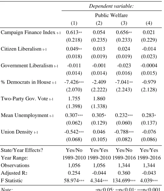
differences remain between the two sets of models. First, due to a discrepancy in the Hamm & Hogan dataset, my information on campaign finance legislation begins in 1989, rather than 1976, though it does extend to 2018 (the model date range is a byproduct of data availability for other covariates). As indicated, perhaps in part due to a corresponding lack of variation in the primary independent variable (fewer overall observations, and a four-point rather than six-point scale), models which include time effects do not produce statistically significant relationships between campaign finance and public welfare spending.10 Additionally, due to data availability/validity concerns I do not report regressions that include demographic information about the racial composition of each state-year, and I use the two-party vote share of the previous Democratic candidate for governor instead of the presence of a Democratic governor and a measure of state party competition. However, the difference in R2 values between our respective analyses
suggests that these changes in model specification represent a substantial decrease in explanatory power. Of note, in models (3) and (4) I drop the measure of governor vote share in an attempt to increase the date range of the balanced panel (as I only have data for that measure through 2010), and observe no substantive difference in the within state or state-time effects models.
Table 2a. Replication of Flavin (Table 1) - Public Welfare
Dependent variable: Public Welfare
(1) (2) (3) (4)
Campaign Finance Index t-1 0.613** 0.054 0.656** 0.021 (0.218) (0.235) (0.233) (0.229) Citizen Liberalism t-1 0.049** 0.013 0.024 -0.014
(0.018) (0.019) (0.019) (0.023) Government Liberalism t-1 -0.011 -0.001 -0.023 -0.0004 (0.014) (0.014) (0.016) (0.015) % Democrats in House t-1 -7.426*** -2.409 -7.041** -0.979
(2.070) (2.222) (2.243) (2.128) Two-Party Gov. Vote t-1 1.755 1.860
(1.398) (1.338)
Mean Unemployment t-1 0.307*** 0.305* 0.232*** 0.283* (0.062) (0.129) (0.060) (0.137) Union Density t-1 -0.542*** 0.046 -0.788*** -0.076
(0.068) (0.105) (0.082) (0.086) State/Year Effects? Yes/No Yes/Yes Yes/No Yes/Yes Year Range: 1989-2010 1989-2010 1989-2016 1989-2016
Observations 1,056 1,056 1,344 1,344
Adjusted R2 0.254 -0.044 0.360 -0.043
F Statistic 58.974*** 4.344*** 134.699*** 4.039***
Note: *p<0.05; **p<0.01; ***p<0.001
implications of these results will be discussed further in the paper. I will note that the models in both of these tables reflect the anticipated importance of the unemployment rate on welfare expenditures––that is, it would appear that welfare expenditures are primarily driven by need, rather than political factors. This is heartening information.
Table 2b. Replication of Flavin (Table 1) - Cash Assistance, Parks and Recreation
Dependent variable:
Cash Assistance Parks and Recreation
(1) (2) (3) (4)
Campaign Finance Index t-1 -0.050 0.049 -0.001 -0.0004 (0.075) (0.075) (0.013) (0.014) Citizen Liberalism t-1 -0.021*** -0.013 -0.002 0.002
(0.006) (0.007) (0.001) (0.002) Government Liberalism t-1 0.014* 0.011 0.003* 0.003* (0.006) (0.006) (0.001) (0.001)
% Democrats in House t-1 1.887** 0.618 0.136 0.141
(0.609) (0.799) (0.193) (0.201)
Two-Party Gov. Vote t-1 -0.296 -0.256 0.071 0.106
(0.437) (0.410) (0.118) (0.116) Mean Unemployment t-1 0.211*** 0.130** -0.020*** -0.007
(0.033) (0.049) (0.005) (0.010)
Union Density t-1 0.163*** 0.005 0.017* 0.002
(0.038) (0.042) (0.007) (0.009)
State/Year Effects? Yes/No Yes/Yes Yes/No Yes/Yes
Year Range: 1989-2008 1989-2008 1989-2010 1989-2010
Observations 912 912 1,056 1,056
Adjusted R2 0.384 -0.027 0.022 -0.048
F Statistic 88.998*** 6.820*** 11.055*** 3.743***
In addition, I then take advantage of the more detailed data at my disposal to investigate a distinction in the causal driver of the relationship observed in Flavin’s results and the models in Table 2a regarding welfare expenditures. Tables 3 and 4 repeat the regressions presented in Table 2a, replacing the modified version of Flavin’s campaign finance index with more granular variables: the dollar amount of limits on campaign contributions to candidates for state
house/assembly from individuals (in Table 3 as I.L.) and PACs (in Table 4 as PAC L.). In following with the original coding scheme of Hamm and Hogan (2008), I operationalize
Table 3. Individual Contribution Limits and Public Welfare
Dependent variable: Public Welfare
(1) (2) (3) (4) (5) (6) (7) (8)
I.L. t-1 -0.000* -0.000 -0.000* -0.000
(0.000) (0.000) (0.000) (0.000)
I.L. (R) t-1 -1.693* -0.536 -1.691* -0.535
(0.765) (0.777) (0.753) (0.751)
Cit. Lib. t-1 0.051** 0.051** 0.013 0.013 0.026 0.026 -0.015 -0.015 (0.019) (0.019) (0.019) (0.019) (0.019) (0.019) (0.022) (0.022) Gov’t Lib t-1 -0.010 -0.010 -0.001 -0.001 -0.023 -0.023 -0.0004 -0.0004 (0.014) (0.014) (0.014) (0.014) (0.016) (0.016) (0.014) (0.014) % Dems. t-1 -6.935*** -6.935*** -2.425 -2.425 -6.606** -6.606** -1.053 -1.053
(2.062) (2.062) (2.218) (2.218) (2.168) (2.168) (2.101) (2.101) Gov. Vote t-1 1.748 1.748 1.926 1.926
(1.421) (1.421) (1.325) (1.325)
Unemp. t-1 0.316*** 0.316*** 0.300* 0.300* 0.239*** 0.239*** 0.274* 0.274* (0.061) (0.061) (0.130) (0.130) (0.060) (0.060) (0.138) (0.138) Unions t-1 -0.520*** -0.520*** 0.044 0.044 -0.768*** -0.768*** -0.080 -0.080
(0.066) (0.066) (0.104) (0.104) (0.080) (0.080) (0.086) (0.086) State/Year
Effects? Yes/No Yes/No Yes/Yes Yes/Yes Yes/No Yes/No Yes/Yes Yes/Yes Year Range:
1989-2010 1989-2010 1989-2010 1989-2010 1989-2016 1989-2016 1989-2016 1989-2016 Observations 1,056 1,056 1,056 1,056 1,344 1,344 1,344 1,344 Adjusted R2 0.256 0.256 -0.041 -0.041 0.360 0.360 -0.041 -0.041 F Statistic 59.540*** 59.540*** 4.731*** 4.731*** 134.887*** 134.887*** 4.560*** 4.560***
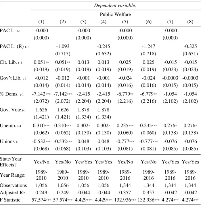
Table 4. PAC Contribution Limits and Public Welfare
Dependent variable: Public Welfare
(1) (2) (3) (4) (5) (6) (7) (8)
PAC L. t-1 -0.000 -0.000 -0.000 -0.000
(0.000) (0.000) (0.000) (0.000)
PAC L. (R) t-1 -1.093 -0.245 -1.247 -0.325
(0.715) (0.632) (0.718) (0.651)
Cit. Lib. t-1 0.051** 0.051** 0.013 0.013 0.025 0.025 -0.015 -0.015 (0.019) (0.019) (0.019) (0.019) (0.019) (0.019) (0.023) (0.023) Gov’t Lib. t-1 -0.012 -0.012 -0.001 -0.001 -0.024 -0.024 -0.0003 -0.0003 (0.014) (0.014) (0.014) (0.014) (0.016) (0.016) (0.015) (0.015) % Dems. t-1 -7.142*** -7.142*** -2.415 -2.415 -6.779** -6.779** -1.054 -1.054
(2.072) (2.072) (2.204) (2.204) (2.216) (2.216) (2.102) (2.102) Gov. Vote t-1 1.626 1.626 1.878 1.878
(1.421) (1.421) (1.334) (1.334)
Unemp. t-1 0.310*** 0.310*** 0.302* 0.302* 0.235*** 0.235*** 0.276* 0.276* (0.062) (0.062) (0.130) (0.130) (0.060) (0.060) (0.138) (0.138) Unions t-1 -0.532*** -0.532*** 0.048 0.048 -0.777*** -0.777*** -0.076 -0.076
(0.068) (0.068) (0.103) (0.103) (0.081) (0.081) (0.085) (0.085) State/Year
Effects? Yes/No Yes/No Yes/Yes Yes/Yes Yes/No Yes/No Yes/Yes Yes/Yes Year Range:
1989-2010 1989-2010 1989-2010 1989-2010 1989-2016 1989-2016 1989-2016 1989-2016 Observations 1,056 1,056 1,056 1,056 1,344 1,344 1,344 1,344 Adjusted R2 0.249 0.249 -0.044 -0.044 0.357 0.357 -0.042 -0.042 F Statistic 57.574*** 57.574*** 4.429*** 4.429*** 132.936*** 132.936*** 4.274*** 4.274***
Table 4 repeats the same analysis, but with limits on PAC campaign contributions. Contrary to the results of an analysis of individual contribution limits, in no model specification presented do limits on PAC contributions independently influence public welfare expenditures. This analysis suggests that, to the extent that campaign finance stringency influences
redistributive expenditures as modeled by Flavin (2015), the portion of the effect driven by contribution limits is more likely due to limits on individual, not PAC, expenditures. I hold further elaboration on this point (including time effects) until the discussion later in this paper.
Mass-Based Approach
The next set of regressions are the result of an investigation of a causal pathway that has been implicitly suggested by the literature (e.g. Bonica et al., 2013; Leighley and Nagler, 2013) but to my knowledge has not yet been empirically tested: that more inclusive electoral
institutions––reforms that make it easier, rather than harder, to vote––are (causally) associated to a more redistributive orientation of state policy. The presumed causal pathway usually goes as follows: if there were to be an exogenous change in electoral institutions in a state that opened up the voting process to more individuals, the composition of the electorate would change to be more representative of the state as a whole. Given that non-voting individuals, on average, have different policy preferences than voting individuals, legislators should respond to changes in the electorate accordingly––for example, by increasing the amount of redistributive spending by the state.
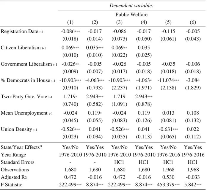
must register in order to vote, ranging from 0 (in other words, election day registration) to 50 (Arizona up until the early 1990’s). Coding decisions for this variable are discussed above, in the discussion of data and methodology, and in a more detailed coding supplement. Model (1) suggests that moving the closing registration date two weeks closer to election day would be associated with around a percentage point increase in the proportion of the budget devoted to public welfare (-0.08 * -14 = 1.12), though this effect disappears with time effects. However, once standard errors are adjusted to reflect serial correlation in the data, there is no evidence to suggest that the coefficient on registration date is statistically different from zero.11 These model specifications include a battery of controls for left party control, party competition, union
strength, and the unemployment rate, as well as state and time effects. As an added measure, I also report the same results using a dummy variable to indicate the presence or absence of
election day registration in Table 6 (i.e., Registration Date of 0), and drop two controls in models (5) and (6) of Table 5. I remove citizen liberalism out of hesitation about the measure’s validity (see footnote in methodology section) and the two-party vote share of the previous Democratic candidate for governor in order to increase the number of years of data available. Again, within state effects and two-way state and time effects models do not produce statistically significant results.
11 To that end, I’ll offer the following haiku, courtesy of Keisuke Hirano and via Angrist and Pischke (2009):
T-stat looks too good Try clustered standard errors––
Table 5. Closing Date for Registration
Dependent variable: Public Welfare
(1) (2) (3) (4) (5) (6)
Registration Date t-1 -0.086*** -0.017 -0.086 -0.017 -0.115 -0.005 (0.018) (0.014) (0.073) (0.050) (0.061) (0.043) Citizen Liberalism t-1 0.069*** 0.035*** 0.069** 0.035
(0.010) (0.010) (0.022) (0.025)
Government Liberalism t-1 -0.026** -0.005 -0.026 -0.005 -0.035 -0.006 (0.009) (0.007) (0.017) (0.018) (0.018) (0.018) % Democrats in House t-1 -10.903*** -4.063*** -10.903*** -4.063* -11.074*** -3.084
(0.910) (0.793) (2.237) (1.971) (2.138) (1.829) Two-Party Gov. Vote t-1 1.719* 2.943*** 1.719 2.943***
(0.740) (0.582) (1.091) (0.878)
Mean Unemployment t-1 -0.024 0.119* -0.024 0.119 0.013 0.108 (0.045) (0.055) (0.083) (0.126) (0.081) (0.132) Union Density t-1 -0.526*** 0.041 -0.526*** 0.041 -0.631*** 0.022
(0.023) (0.034) (0.055) (0.113) (0.065) (0.112) State/Year Effects? Yes/No Yes/Yes Yes/No Yes/Yes Yes/No Yes/Yes Year Range 1976-2010 1976-2010 1976-2010 1976-2010 1976-2016 1976-2016
Standard Errors - - HC1 HC1 HC1 HC1
Observations 1,680 1,680 1,680 1,680 1,968 1,968
Adjusted R2 0.472 -0.016 0.472 -0.016 0.530 -0.033
F Statistic 222.499*** 8.874*** 222.499*** 8.874*** 453.379*** 5.842***
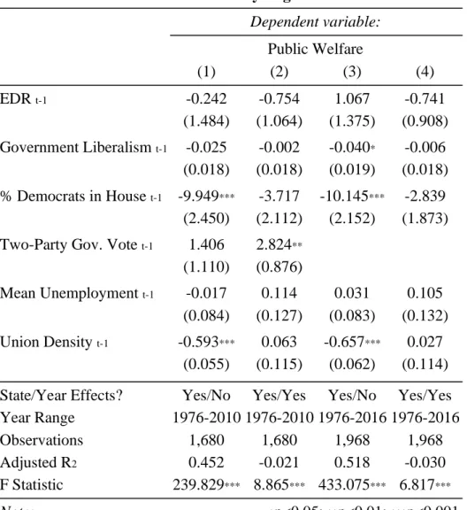
Table 6. Election Day Registration
Dependent variable: Public Welfare
(1) (2) (3) (4)
EDR t-1 -0.242 -0.754 1.067 -0.741
(1.484) (1.064) (1.375) (0.908) Government Liberalism t-1 -0.025 -0.002 -0.040* -0.006
(0.018) (0.018) (0.019) (0.018) % Democrats in House t-1 -9.949*** -3.717 -10.145*** -2.839
(2.450) (2.112) (2.152) (1.873) Two-Party Gov. Vote t-1 1.406 2.824**
(1.110) (0.876)
Mean Unemployment t-1 -0.017 0.114 0.031 0.105 (0.084) (0.127) (0.083) (0.132) Union Density t-1 -0.593*** 0.063 -0.657*** 0.027
(0.055) (0.115) (0.062) (0.114) State/Year Effects? Yes/No Yes/Yes Yes/No Yes/Yes Year Range 1976-2010 1976-2010 1976-2016 1976-2016
Observations 1,680 1,680 1,968 1,968
Adjusted R2 0.452 -0.021 0.518 -0.030
F Statistic 239.829*** 8.865*** 433.075*** 6.817***
Note: *p<0.05; **p<0.01; ***p<0.001
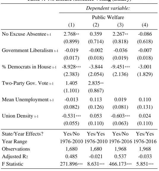
Table 7. No Excuse Absentee Voting (Binary)
Dependent variable: Public Welfare
(1) (2) (3) (4)
No Excuse Absentee t-1 2.768** 0.359 2.267** -0.086 (0.899) (0.714) (0.818) (0.618) Government Liberalism t-1 -0.019 -0.002 -0.036 -0.007
(0.017) (0.018) (0.019) (0.018) % Democrats in House t-1 -8.928*** -3.844 -9.451*** -3.001
(2.383) (2.054) (2.136) (1.829) Two-Party Gov. Vote t-1 1.405 2.835**
(1.101) (0.867)
Mean Unemployment t-1 -0.013 0.113 0.019 0.110 (0.082) (0.126) (0.081) (0.131) Union Density t-1 -0.531*** 0.053 -0.603*** 0.024
(0.055) (0.110) (0.063) (0.110) State/Year Effects? Yes/No Yes/Yes Yes/No Yes/Yes Year Range 1976-2010 1976-2010 1976-2016 1976-2016
Observations 1,680 1,680 1,968 1,968
Adjusted R2 0.485 -0.021 0.537 -0.033
F Statistic 271.896*** 8.631*** 466.173*** 5.851***
Causal Mechanism: Electoral Class Bias
In the pages that follow I draw on Franko et al.’s measure of “Electoral Class Bias” to investigate further the presumed causal relationship––that is, that these policy changes might occur because they are associated with changes in the composition of the electorate.12 As
described above (and further in the appendix), this CPS and regression-generated measure can be thought of as the difference in probability of voting of the lowest and highest income groups in each state. As stated by the authors, “A value of 0.33 (the average of the measure across all years and states), for example, indicates that the rich are 33% more likely to vote than the poor”
(Franko et al. (2016), Appendix A). This relationship offers an opportunity to better understand whether the “mass-based” effects (and lack thereof) presented above are due to a lack of change in the electorate or some other set of factors.
In Tables 8 and 9, I present results of a within state effects OLS regression using a lagged independent variable for the effect of the closing date for registration and no-excuse absentee voting on electoral class bias. I lag the independent variable for both one and two time periods to allow for the possibility that a change in law takes time to be reflected in changes in the
electorate. Of note, in no regression specification does the election policy have a significant effect on the composition of the electorate once controlling for income per capita,
unemployment, and union participation. Of note, in both cases it would appear that increased unemployment significantly drives up the levels of income bias in the electorate.
12 I want to especially thank Prof. Nathan Kelly, who generously provided me access to this measure, developed for Franko, W. W., Kelly, N. J., & Witko, C. (2016). Class Bias in Voter Turnout, Representation, and Income
Table 8. Registration Date and Electoral Class Bias
Dependent variable: Electoral Class Bias
(1) (2) (3) (4)
Registration Date t-1 -0.107 -0.030
(0.059) (0.052)
Registration Date t-2 -0.108 -0.044
(0.057) (0.055)
Income per Capita t-1 -0.0003 -0.0003
(0.0003) (0.0003)
Mean Unemployment t-1 0.869*** 0.879***
(0.202) (0.200)
Union Density t-1 -0.060 -0.068
(0.140) (0.142) State/Year Effects? Yes/No Yes/No Yes/Yes Yes/Yes Year Range 1976-2006 1976-2006 1976-2006 1976-2006
Observations 1,470 1,421 1,470 1,421
Adjusted R2 -0.028 -0.029 -0.025 -0.026
Table 9. Absentee Voting and Electoral Class Bias
Dependent variable: Electoral Class Bias
(1) (2) (3) (4)
No Excuse Absentee t-1 1.122 0.754
(1.053) (1.017)
No Excuse Absentee t-2 0.943 0.620
(1.048) (1.037)
Income per Capita t-1 -0.0002 -0.0002
(0.0003) (0.0003)
Mean Unemployment t-1 0.876*** 0.878***
(0.206) (0.206)
Union Density t-1 -0.073 -0.070
(0.139) (0.139) State/Year Effects? Yes/No Yes/No Yes/Yes Yes/Yes Year Range 1976-2006 1976-2006 1976-2006 1976-2006
Observations 1,519 1,519 1,470 1,470
Adjusted R2 -0.052 -0.053 -0.025 -0.025
F Statistic 3.360 2.274 11.461*** 11.332*** Note: *p<0.05; **p<0.01; ***p<0.001
Discussion
and am unable to reject the null hypothesis that these reforms have no influence on the composition of the electorate. However, once time effects are included, I cannot conclusively make statements about either the relationship Flavin (2015) observes or that predicted by the literature on voter and non-voter preferences.
The theoretical framework set up over the course of this paper suggests that these relationships are causal––states with later registration dates have higher redistributive
expenditures, all else equal, because those later registration dates in some way alter legislator’s incentives. And while various model decisions have been made in such a way as to facilitate that understanding––lagging the independent variable and employing a within-effects panel data approach, for example––the claim of causality is not as clear-cut as it might be were an exogenous shock (such as, say, a court case) to be the driver of this analysis. Certainly, the evidence that these reforms may not alter the composition of the electorate in a meaningful way suggests that a careful reconsideration of that mechanism may be in order. Additionally, the knowledge that controlling for time trends across all states removes the significance of the hypothesized relationship should be a cause of serious doubt. Below, I offer a few interpretations of the results presented above, revisit the conclusions of the literature in light of this information, and touch on the policy implications of this work.
The lack of a crystal-clear picture across all model specifications allows some room for various interpretations of the regressions above, and so I offer two: one based on models that do not include time effects, and one based on a more complete model specification that does. At the very least, barring the inclusion of time effects, it would appear that more stringent campaign finance law and no-excuse absentee voting are associated with higher public welfare
relationship viewed through within state fixed and random effects.13 Even if this were the case, we would still need to reconsider the statement that this latter relationship is due to changes in the composition of the electorate, at least on an income dimension, in light of the information presented in Tables 8 and 9. Are there still mechanisms by which these institutions might affect legislator behavior if not by directly altering the electorate, and consequently, who sat in state office? In short, perhaps. One could feasibly imagine that legislators might not only be responsive to votes at the ballot box, but also to perceptions of who might vote, in particular when the exact income composition of the electorate is not clear (i.e., when the best information we can rely on are exit polls and CPS/ANES estimates). Additionally, if the knowledge that election day registration is possible were to encourage increased political participation outside of voting from previously less-active populations, we might encounter a similar effect.
However, the knowledge that these effects are not robust to the inclusion of time effects should give us serious pause in this line of thinking. In the models above, I do not find any political variables that are consistently associated with public welfare expenditures in U.S. states. This is a surprising finding, for several reasons. First, it would appear to cast doubt on the causal assurance offered by the models presented in Flavin (2015) that demonstrate a relationship between campaign finance stringency and public welfare expenditures. Our estimation strategies are not wildly divergent: while the time periods covered are different, they represent only a minimal difference in time frame (27 years vs. 32 years); for the years in which they overlap, a four-point and six-point campaign finance index correlate at nearly 0.8; and both use standard error adjustments common in applications of cross-sectional time series data (MacKinnon and
White heteroscedasticity and autocorrelation consistent “clustered” standard errors, and Beck and Katz panel corrected standard errors). Additionally, while findings with state effects support statements that suggest reforms such as no-excuse absentee voting would increase redistributive expenditures, the lack of findings with time effects and inability to demonstrate the proposed mechanism call into question the empirical backing for those claims.
Why might this be the case? Two insights from Rigby and Springer (2011) may help to guide discussion. The authors examine the effects of five electoral reforms––mail-in registration, motor voter (registration at the DMV/MVA), election day registration, no excuse absentee voting, and early voting––on the income bias of registration rolls and of the electorate (CPS data). Of note for this study, they distinguish between three kinds of electoral reforms: those that improve the ease of registration, those that eliminate the registration process all-together, and those that make voting more convenient. Additionally, they find that motor-voter laws and election day registration decrease electoral income bias when registration rolls were highly unequal prior to the reform, and that early voting had a net positive increase on income bias in situations of prior high registration bias. This interaction effect suggests that, when these institutional changes do have a visible effect, they do because the environment is particularly conducive to the kind of change in behavior they would elicit. That is, if the closing date for registration were to alter the electorate (or, as mentioned above, perceptions of the electorate), it might be more likely to do so when the electorate was already highly unrepresentative of the general population and there was more room for a substantial change due to the reform.
less likely to expect to see changes in redistributive policy, despite increases in turnout. Future studies with access to registration data (or estimates thereof) might take such an approach.
This study examined the effects of two varieties of electoral institutions on a polarizing expenditure category. Turnout-increasing institutions such as absentee voting and later
Appendix:
Electoral Class Bias
The following description of the construction of the Electoral Class Bias measure used in this paper is an excerpt from Appendix A of Franko, W. W., Kelly, N. J., & Witko, C. (2016). Class Bias in Voter Turnout, Representation, and Income Inequality. Perspectives on Politics, 14(2), 351–368. Again, I want to extend serious thanks to Prof. Nathan Kelly for allowing me to access this data.
“We draw on the Current Population Survey (CPS) Voter Supplements to construct our measure of electoral class bias (Brown et al. 1999; Hill and Leighley 1992; Rigby and
Springer 2011; Rosenstone and Hansen 1993)…The CPS interviews thousands of individuals in
every state allowing for representative estimation of turnout rates in each state, even in those states with small populations. [And], questions about voting have been consistently asked for
each presidential and midterm election for several decades…
Our measure captures disproportionate participation rates across income groups (Blakely et al. 2001; Mackenbach and Kunst 1997; Wichowsky 2012), providing an empirical measure of how much richer citizens participate in elections relative to others within their state. The class bias variable is created by first assigning all CPS respondents to a cumulative, within-state family income distribution. For instance, consider a CPS respondent who reports a family
income of $50,000 to $59,999. If this income category consists of 10% of the state’s residents
and 50% of the population falls below this income level, then this individual is assigned to 0.55
on the state’s cumulative income distribution (0.50 + [0.10/2]). This within state income position
is then used as a determinant of voter turnout in the following OLS regression model:
vote = b0 + b1(income position) + e,
where vote is coded as 1 if the individual reported voting and 0 if the person did not vote, and income position indicates each individual’s position on their state’s cumulative income
distribution as described above. A unique regression model is specified for each state and each election year. Since both variables (vote and income) are bounded between 0 and 1, the resulting coefficient (b1) on the cumulative income scale is interpreted as the absolute difference in the
probability of voting for the poorest and richest income group in each state…
Figure A1: Growth of Top 1% Income Share in the United States
Figure A2: Smoothed Changes in Employment and Hourly Wages, 1980-2005
Figure A3. DV: Electoral Class Bias
Figure A5. Closing Date for Registration
Table A1. Covariate Correlation Matrix
Gov’t Liberalism
% Dems. in House
Gov.
Vote Share Unemployment
Union Density
Gov’t Liberalism 1 0.090 0.159 0.102 0.067
% Dems. 0.090 1 0.334 0.261 0.181
Gov. Vote Share 0.159 0.334 1 0.180 0.103
Unemployment 0.102 0.261 0.180 1 0.292
Table A2. Descriptive Statistics
N Mean St. Dev. Min Max Year Range
Public Welfare 1,450 21.82 5.27 6.68 38.78 1970 - 2017
Cash Assistance 1,000 1.58 1.13 0.00 6.63 1970 - 2008
Parks and Recreation 1,450 0.44 0.30 0.04 4.00 1970 - 2017
ECB Index 1,550 34.01 7.67 10.77 67.74 1976 - 2006
Campaign Finance Index 1,450 2.65 1.10 0 4 1989 - 2017
Individual Limits 1,450 290,198.70 452,654.60 0 1,000,000 1989 - 2017 Individual Limits (Rescaled) 1,450 0.29 0.45 0 1 1989 - 2017 PAC Limits 1,450 340,257.70 472,248.90 0 1,000,000 1989 - 2017
PAC Limits (Rescaled) 1,450 0.34 0.47 0 1 1989 - 2017
Registration Date 1,450 21.15 10.83 0 50 1976 - 2017
Election Day Registration 1,450 0.13 0.34 0 1 1976 - 2017
No-Excuse Absentee 1,450 0.43 0.49 0 1 1970 - 2017
Citizen Liberalism 1,372 50.11 15.32 8.45 97.00 1970 - 2016 Government Liberalism 1,421 47.40 14.64 17.51 73.62 1970 - 2017
% Dems. in House 1,372 0.52 0.17 0.13 0.93 1970 - 2016
Dem. Governor Vote Share 1,078 0.49 0.11 0.11 0.82 1970 - 2010 Unemployment Rate (Mean) 1,450 5.56 1.82 2.30 13.61 1976 - 2017
Union Density 1,450 12.24 5.88 2 30 1971 - 2017
Bibliography:
Acemoglu, D., and Robinson J. A. (2012). Why Nations Fail: The Origins of Power, Prosperity and Poverty (1st ed.). New York: Crown Publishers, c2012.
Alvaredo, F., Atkinson, A. B., Piketty, T., & Saez, E. (2013). The Top 1 Percent in International and Historical Perspective. Journal of Economic Perspectives, 27(3), 3–20.
https://doi.org/10.1257/jep.27.3.3
Avery, J. M. (2015). Does Who Votes Matter? Income Bias in Voter Turnout and Economic Inequality in the American States from 1980 to 2010. Political Behavior, 37(4), 955–976.
https://doi.org/10.1007/s11109-015-9302-z
Ballard-Rosa, C., Martin, L., & Scheve, K. (2016). The Structure of American Income Tax Policy Preferences. The Journal of Politics, 79(1), 1–16. https://doi.org/10.1086/687324
Beck, N., & Katz, J. N. (1995). What To Do (and Not to Do) with Time-Series Cross-Section Data. American Political Science Review, 89(3), 634–647. https://doi.org/10.2307/2082979
Berry, W. D., Ringquist, E. J., Fording, R. C., & Hanson, R. L. (1998). Measuring Citizen and Government Ideology in the American States, 1960-93. American Journal of Political Science, 42(1), 327–348. JSTOR. https://doi.org/10.2307/2991759
Berry, W. D., Fording, R. C., Ringquist, E. J., Hanson, R. L., & Klarner, C. E. (2010). Measuring Citizen and Government Ideology in the U.S. States: A Re-appraisal. State Politics & Policy Quarterly, 10(2), 117–135. https://doi.org/10.1177/153244001001000201
Berry, W. D., Fording, R. C., Ringquist, E. J., Hanson, R. L., & Klarner, C. (2013). A New Measure of State Government Ideology, and Evidence that Both the New Measure and an Old Measure Are Valid. State Politics & Policy Quarterly, 13(2), 164–182.
https://doi.org/10.1177/1532440012464877
Bonica, A., McCarty, N., Poole, K. T., & Rosenthal, H. (2013). Why Hasn’t Democracy Slowed Rising Inequality? Journal of Economic Perspectives, 27(3), 103–124.
https://doi.org/10.1257/jep.27.3.103