Gravitational Radiation in
f
(
R
)
Gravity: A Geometric
Approach
Adam Scott Kelleher
A dissertation submitted to the faculty of the University of North Carolina at Chapel
Hill in partial fulfillment of the requirements for the degree of Doctor of Philosophy
in the Department of Physics and Astronomy.
Chapel Hill
2013
Approved by:
Laura Mersini-Houghton
Y. Jack Ng
Charles Evans
Dmitri Khveshchenko
Ryan Rohm
Abstract
ADAM SCOTT KELLEHER: Gravitational Radiation inf(R)Gravity: A Geometric Approach.
(Under the direction of Laura Mersini-Houghton.)
I summarize experimental and theoretical constraints on gravity theories. I explore metric f(R)
gravity, and explore scalar field theory analogs. I present a different kind of mechanism to raise the
effective scalar mass in f(R) gravity in environments with particular ranges of background scalar
curvatures, and thus suppress scalar effects on solar system curvature scales, while allowing scalar
effects at different curvature scales. I review the post-Newtonian and post-Minkowskian
mathemat-ical machinery for General Relativity, and generalize these expansions to metric f(R) gravity up to
Dedicated to Bill Walsh, a true brother.
Acknowledgments
I would like to thank my brother for his support, Bart Dunlap and Greg Herschlag for useful
conversations, and my advisor Laura Mersini-Houghton for her guidance. I thank the Department
Table of Contents
List of Figures . . . viii
List of Abbreviations and Symbols . . . ix
1 Introduction . . . 1
2 Properties of Gravity Theories . . . 4
2.1 Equivalence Principles . . . 4
2.2 Metric Theories of Gravity . . . 6
2.3 PPN Formalism and Experimental Constraints . . . 8
2.3.1 PPN Parameters . . . 8
2.3.2 Experimental Constraints on Gravity Theories . . . 10
2.4 Constraints from Pulsar Data . . . 15
3 Tensor-Scalar Gravity . . . 16
3.1 Tensor Multi-Scalar Theory . . . 18
3.1.1 Action and Field Equations . . . 18
3.1.2 Radiation Sources . . . 19
3.2 Tensor-Scalar Theory: Brans-Dicke with Potential and Variableω. . . 21
3.2.1 Variation of Newton’s Constant . . . 22
3.2.2 Effect of Potential . . . 22
3.3 Brans-Dicke without Potential with Constantω . . . 22
3.4 The Chameleon Mechanism . . . 23
4 f(R)Gravity . . . 28
4.1 Basic Theory . . . 28
4.2 Problems with Palatini . . . 29
4.2.1 Metric algebraically related to energy-momentum . . . 29
4.2.2 Background-dependent Newtonian Limit . . . 30
4.3 Properties of Metricf(R) Gravity . . . 30
4.3.1 Equivalence off(R) and Scalar-Tensor Gravity . . . 31
4.3.2 Chameleon Mechanism inf(R) Gravity . . . 33
4.3.3 Theoretical Constraints . . . 33
5 Series Expansion Solutions in Gravity . . . 37
5.1 Overview . . . 37
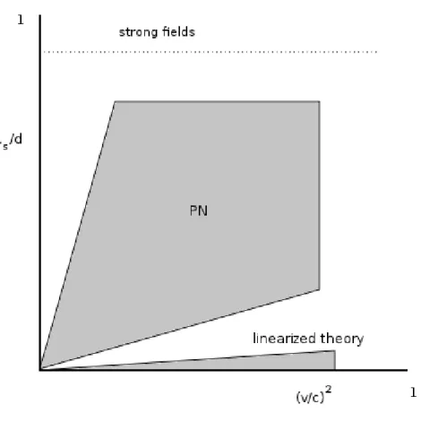
5.1.1 Series Solutions and Matching . . . 38
5.2 The Post-Newtonian Expansion . . . 40
5.3 Linearized Gravity . . . 43
5.3.1 In General Relativity . . . 43
5.3.2 In Scalar-Tensor Gravity . . . 44
5.3.3 In f(R) Gravity . . . 45
5.4 The Post-Minkowskian Expansion . . . 45
5.4.1 In General Relativity . . . 46
5.4.2 In f(R) Gravity . . . 48
6 New Phenomena Near Critical Points . . . 51
6.1 Discontinuous Case . . . 52
6.2 Continuous Case . . . 54
6.3 New Phenomena Nearf00(R) = 0 . . . 57
6.4 Conclusions . . . 62
7 Post-Newtonian Equations . . . 64
7.1 Set-Up . . . 64
7.2 Solution . . . 66
8 Post-Minkowskian Equations . . . 69
8.1 Set-Up . . . 69
8.1.1 Identities . . . 70
8.2.1 Einstein Tensor . . . 70
8.2.2 Effective Source . . . 70
8.2.3 Trace Equation . . . 71
8.2.4 Field Re-definition . . . 72
8.2.5 Results . . . 74
9 Conclusions . . . 76
9.1 Summary . . . 76
9.2 Further Research . . . 77
A Einstein Tensor in f(R)Gravity to 2nd Order . . . 78
List of Figures
2.1 Diagram for Cassini experiment . . . 12
2.2 Diagram of perihelion shift . . . 14
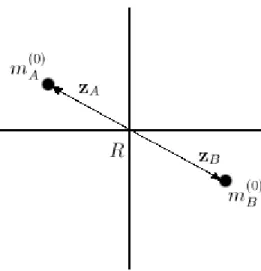
3.1 Our coordinates are in the center-of-mass frame for the two-body system. . . 20
3.2 A potential for the Chameleon mechanism . . . 24
3.3 A schematic effective potential for the Chameleon mechanism . . . 24
3.4 Qualitative weak response of the scalar field to a mass distribution . . . 26
3.5 Qualitative strong response of the scalar field to a mass distribution . . . 26
5.1 Domains of validity for different series expansions . . . 38
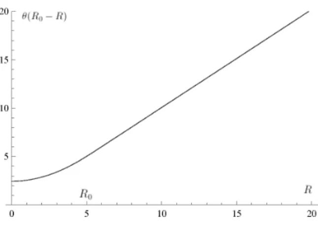
6.1 A displacedθfunction,θ(R0−R). . . 52
6.2 A displacedθfunction,θ(R−R0). . . 52
6.3 A reflected, displacedθfunction,θ(R0−R). . . 53
6.4 Anf(R) with a critical point . . . 53
6.5 The functionf(R), where aboveR0the theory is like GR. BelowR0, there is another scalar degree of freedom. . . 54
6.6 An approximateθfunction . . . 55
6.7 The differentiable function,f(R). . . 56
6.8 A differentiablef(R) with critical point effects . . . 58
6.9 Effective scalar field mass near critical points . . . 61
6.10 A right-moving wave heads toward the boundary, near x= 10. . . 61
6.11 The wave gets partially deflected as it approaches the boundary. . . 61
List of Abbreviations and Symbols
i, j, k, . . . Spatial coordinates indices running from 1 to 3
µ, ν, α, . . . Space time coordinates indices running from 0 to 3
gµν The components of the metric tensor
Rµναβ The components of the Riemann tensor
Rµν The components of the Ricci tensor
R The scalar curvature
ηµν The Minkowski metric
φ, ϕ Scalar field n
hµν Thenth order part ofhµν in some expansion
Γαµν The components of the Christoffel connection
hµν A perturbation to the metric, wheregµν =ηµν+hµν
g The determinant of the metric tensor,gµν
h The approximate trace of the metric perturbation,h=ηµνh µν
x A spatial 3-vector in a post-Newtonian coordinate system
ˆ
n A spatial unit 3-vector in a post-Newtonian coordinate system
Chapter 1
Introduction
General Relativity has been a great success in explaining phenomena that were not covered by
Newtonian gravity. Its major historical successes included explaining the perihelion shift of Mercury,
and properly calculating the lensing due to the Sun. It correctly reduces to Newtonian gravity in
the low energy, low velocity limit, and thus agrees with past experiments in Newtonian physics.
As time went on, there were still more observations that could not be explained. As early as
1933, Zwicky [1] posed the “missing mass” problem for galaxy clusters, an early version of the dark
matter problem. In 1975 the problem took on its well known form. The announcement was made
at an AAS meeting that stars in spiral galaxies orbited with roughly the same speed, based on
measurements with a new, more sensitive spectrograph [2]. The observations have been attributed
to a yet-unobserved type of matter, now known as dark matter.
In addition to the dark matter problem, the universe was observed to be accelerating its expansion
in 1998, by examining luminosity data of Type Ia supernovae [3][4]. This could be accounted for in
the context of GR by introducing a cosmological constant, but that brought about a host of other
problems. The “coincidence problem”, for example, is the question“Why do we exist during the
relatively brief period in the history of the universe when the vacuum energy density is comparable
to the matter energy density?”. Then, there is the magnitude problem. From particle theory
considerations, the vacuum energy should be as much as 120 orders of magnitude larger than that
observed [5][6]. Thus, the accelerated expansion of the universe can not yet be explained with
particle theories in a way that is consistent with General Relativity (GR).
These observations lead to attempts at resolving them that typically involve either modifications
to gravity (the geometric part of the action), or introducing new dynamic fields (the matter part of
the action). By having a dark energy that can evolve with time, the coincidence problem can be
avoided.
It is difficult to motivate the fact that extra fields should not couple to matter, as there is no
symmetry to prevent this. It is also difficult to explain why the particle mass in dark energy theories
should be so small. Thus, one could argue [7] that modified gravity theories are better motivated
I prefer, then to look at modified gravity theories over particle theories. A particularly interesting
class of theories is metric f(R) gravity. While this class of theories hasn’t been very successful at
explaining dark matter1, it has some promise for dark energy2.
The theory effectively introduces a scalar field that only interacts with matter in combination
with the gravitational field, so is rather similar to scalar field models of dark energy, but introduces
no actual new matter fields. Thus, it has the strengths of particle theories of dark energy, but
without the field-theory-based weaknesses. It is also theoretically interesting that other theories, or
quantum corrections can introduce higher order curvature invariants [15, 16], and higher invariants
can allow the theory of gravity to be renormalizable [17, 18]. All of this should be reason enough to
motivate an investigation intof(R) gravity, but we can do even better. It turns out that it really is
the best option for generalizing GR.
One could ask what other types of modifications we could make to the gravitational action. It
turns out that the form of the Lagrangian is very constrained. We’ll go into detail on this when
we address theoretical constraints on f(R) gravity, but it turns out that we can only make the
generalization that the action can contain some function of the Ricci scalar (hence the name,f(R)
gravity). Any other generalization would cause the theory to become unstable [19].
We are left, then, with the option to generalize gravity to f(R) gravity. It should be done in a
way that agrees with all past tests of GR and Newtonian gravity, and in a way that is theoretically
sound and observationally distinguishable from other theories. From one perspective, you could
talk about modifying gravity to be different from GR at particular curvature scales. For example,
f(R) = R+αR2 is like GR with f(R) = R as we move from R = 0 to larger R, but we pick
up modifications when R ∼ 1/α. We could also produce modifications at low curvatures, like
f(R) =R+α/R. Theα/Rterm dominates at lowerR, butf(R) transitions over to being dominated
by the GR term whenR∼√α.
In the next chapter, I will go into detail on the established properties of gravity theories, and give
some understanding of how these properties were established. If a theory is viable, it should fit all of
these constraints on the energy scales where these experiments were performed (typically, in systems
with energy densities and gravitational potentials no greater than the Sun’s). In the Chapter 3, I will
1Sotiriou [8] points out that the roughly quadratic modifications to the Einstein-Hilbert action found by fitting
f(R) =Rnbased on galactic rotation curves [9, 10, 11, 12] contrast with bounds found by Barrow and Clifton[13, 14]
2Sotiriou shows that modifications to the action inf(R) theory can come into the Friedman equations effectively
as a perfect fluid. It is easy to choosef(R) such that the equation of state parameter for this fluid is that of dark energy,wef f =−1 [8].
give some theoretical background on a class of modifications to gravity called scalar-tensor theories.
Here is where I will establish interesting physical phenomena that arise in these theories, many of
which will have analogs inf(R) gravity. I will also describe mechanisms that have been used in the
past to make these theories agree with past observations, but which also render these theories rather
uninteresting and untestable.
In the Chapter 4, I will go into detail onf(R) gravity theories. With all of this set up, we will be
ready to start finding solutions for gravitational phenomena (in particular, gravitational radiation) in
f(R) gravity. Thus, Chapter 5 introduces the mathematical machinery of series expansion solutions
in GR, and explains the state of the art inf(R) gravity (which has been minimal).
With all of the groundwork laid, I’ll start working out solutions forf(R) gravity: In the chapter
6, I describe new phenomena I’ve discovered inf(R) gravity near critical points, where the theory
approaches GR. I believe these new phenomena should lead to clear observable predictions. In
Chapter 7, I develop the post-Newtonian series expansion for f(R) gravity, and in Chapter 8 I
develop the post-Minkowskian series expansion. I show that the post-Minkowskian expansion can
Chapter 2
Properties of Gravity Theories
2.1 Equivalence Principles
There are certain properties of gravity theories that have been verified to high experimental
precision, and should be included in any theory of gravity. Equivalence principles are one such
feature. We will generally follow the excellent explanation of Will, [20], to explain the concept and
the experiments supporting it. At it’s most basic level, the weak equivalence principle (WEP) states
that the property of matter that determines its response to an applied force, or “inertial mass”, is
equal to the quantity determining its acceleration due to gravity, or “passive gravitational mass”.
Phrased differently, we can say write Newton’s second law as
F =mIa, (2.1.1)
and the law of gravitation as
F =mPg. (2.1.2)
Then the WEP states thatmP =mI, so that a=g for any body [21]. That is, bodies accelerate
with the same acceleration in a gravitational field, independent of their masses or compositions.
This has been confirmed experimentally to very high precision. The basic idea is that if some energy
contributes differently to inertial and passive masses, then that difference can be parameterized
approximately as
mP =mI +
X
a
ηaE
a
c2 , (2.1.3)
where ηa parameterizes the contribution from the ath type of internal energy, Ea. Typically we
measure relative differences in acceleration, the “E¨otvos ratio”,
η≡2|a1−a2|
|a1+a2|
=X a
ηa
Ea
1
m1c2
− E
a
2
m2c2
. (2.1.4)
Thus, given the various Ea for a pair of bodies, measurements ofη put upper limits on the ηa.
resultsη = 10−11andη= 10−11, respectively. We have various forms for theEa due to the strong,
electromagnetic, and weak forces. For example, consider the electrostatic nuclear energy in platinum
and aluminum. A semi-empirical formula for the approximate internal energy is
EES
mc2 = 7.6×10
−4Z(Z−1)A−4/3, (2.1.5)
whereZ is the atomic number, andAis the mass number. The difference in this quantity between
platinum and aluminum is 2.5×10⁻³. Simplifying the formula for η to only include the internal
electrostatic force, we can get an upper limit onηa(the case where the entire quantityη is from this
energy contribution) of|ηES| <4×10⁻¹⁰ [20]. Similar considerations can be applied to the other
electromagnetic internal energy contributions, as well as the strong and weak forces.
With strong empirical support for the WEP, we should choose a theory of gravity where the WEP
is either violated very little (smallη), or we could choose it to be a guiding principle, restricting our
consideration of viable theories to ones where η≡0. Metricf(R) gravity is a theory in the second
group.
The WEP implies that all test bodies follow the same free fall paths, independent of their
compositions. This suggests a kind of universality of motion in different reference frames: in any
particular free-falling reference frame, the laws of physics are the same. One can postulate, as
Einstein did, that we can treat these reference frames as inertial frames: they are as good as the
constant-velocity frames of motion in special relativity. More precisely, the laws of physics (e.g.
electromagnetism, mechanics, nuclear decay, etc.) inside of a freely falling elevator will be the same
as those inside an orbiting spacecraft, or one floating in the vacuum of space. This postulate,
together with the WEP, are known as the Einstein equivalence principle, or the EEP.
Since the laws of physics must be the same in different inertial frames, we should be able to
transform from one frame to another at the same space-time point. Thus, Local Lorentz Invariance
(LLI) should exist in any theory of gravity that obeys the EEP. It is difficult to find a “clean” test of
LLI: could the apparent differences in forces be due to unknown physical phenomena? In the past,
apparent LLI-violating effects have been confused with unknown particle interactions. For example,
violation of 4-momentum conservation in beta decay was found to be caused by the emission of a
new particle: the neutrino [20]. The Hughes-Drever experiment is one experiment where LLI has
been tested in a “clean” way, as we will now describe.
a particle due to its state of motion relative to some absolute frame, then that difference can be
quantified as
δmij ∼
X
a
δaE
a
c2 , (2.1.6)
where δmij represents the anisotropic part of the inertial mass quadrupole moment, mij, and δa
parameterizes the contribution to the anisotropy due to the energyEa from the interactiona.
This experiment was performed using 7Li in the J = 3/2 ground state in an external magnetic
field. In the absence of external perturbations, the state is split into 4 equally spaced energy
levels. Perturbations with a non-vanishing quadrupole moment ruins the equality of the energy level
spacing. Using nuclear magnetic resonance techniques, the change in line spacing was constrained
to less than 1.7×10⁻¹⁶eV. The result is that δm
ij <1.7×10⁻¹⁶eV. This implies constraints on
the variousδa for different fundamental interactions of
|δstrong| < 10−23
|δelectrostatic| < 10−22
|δweak| < 5×10⁻¹⁸.
The extremely high precision of these results has lead to the Hughes-Drever experiment being
called the “most precise null experiment ever performed” [20]. This clearly suggests that LLI should
be a requirement of any viable theory of gravity, and lends evidence that the EEP comprises a good
set of postulates on which to build a theory of gravity.
One can make convincing arguments (see [20]) that the EEP implies that the correct theory of
gravity must be a “metric” theory of gravity. We will now describe the properties of metric theories
of gravity.
2.2 Metric Theories of Gravity
A metric theory of gravity is defined as one where
1. space-time is endowed with a metric,g,
2. test bodies’ worldlines are geodesics ofg, and
3. in local free-falling frames (local Lorentz frames), the laws of physics are those of special
relativity.
GR is clearly a metric theory of gravity since it is Lorentz covariant, the Einstein equations
de-scribe how the presence of matter generatesg, and the divergence of these equations produces
equa-tions of motion that reduce, in the case of test particles, to the equaequa-tions for space-time geodesics.
It’s less obvious that gravity theories with other gravitational fields than the metric field are metric
theories of gravity. The trick is in realizing that was long as matter doesn’t couple independently to
the extra fields, the metric alone determines the trajectories of matter. The role of extra
gravita-tional fields is that of determining how matter generates curvature. Indeed, they do enter into the
Einstein equations. The trajectories of test particles, however, are still determined by the geodesic
equation for the metric. We can illustrate this point by looking at scalar-tensor theory, which is
equivalent to a subset of metric f(R) gravity theories. Examining the field equations in different
conformal frames makes the point clear. The difference between the “Jordan” and “Einstein” frames
amounts to a transformation of the scalar field space and conformal transformation of the metric. I
should emphasize that a conformal transformation of the metric is a transformation to a physically
different space-time. The use of performing a conformal transformation on a particular action is
that it can be transformed into a form that is easily manipulated, and can be transformed back by
reversing the conformal transformation.
The “Jordan frame” action is defined as theφ-coordinate frame where the gravitational coupling
to theφfield is of the formφR,
SJ=κ
Z
d4xp−˜g(φR˜−1
2g µν∂
µφ∂νφ−V(φ) +Lm(ψ,g˜µν)), (2.2.1)
and the divergence of the Einstein field equations in this frame is
˜
∇µT˜µν= 0, (2.2.2)
which amounts to the same equations of motion as in general relativity. This means that test
particles follow the geodesics of the metric,gµν.
The Einstein frame action is defined as the φ-coordinates where the gravitational action takes
the formR, and so theφfield doesn’t couple to the scalar curvature in the action. It is written
SE=κ
Z
d4x√−g∗(R∗−1
2g µν
and the divergence of the Einstein equations in this frame is [24]
∇∗νT∗µν =α(φ)T∗∇µ
∗φ. (2.2.4)
Fujii and Maeda dedicate an appendix [25] to showing in detail that it is indeed the fact that φ
enters into the matter action that causes the energy-momentum tensor to no longer be
divergence-less. The basic idea is that if you add a coupling between the φ field and a matter current, J,
to the Lagrangian, Lm → Lm+φJ, then you end up changing the covariant conservation law to
∇µTµν =φ∇νJ. Thus, we needJ = 0 to have a covariant conservation law. The conservation law
is obeyed if and only if particles follow geodesics, which are properties of space-time and not the
particles. Thus, universality of free-fall is maintained, and the WEP is obeyed.
The situation is different in the Einstein frame. We lose the covariant conservation law, so
particles no longer follow geodesics. Instead, they follow pathsuµ∗ satisfying
Duµ∗ Dτ∗
=ζ(uλ∗∂λσ)uµ∗−g∗µλ∂λ(u∗νuν∗)
(2.2.5)
where ζ−2 = 6 + 4ω, and σ is defined by φ = 2√ωeζσ. While these paths are not space-time
geodesics, they are still independent of the particle composition (e.g. particle mass is absent from
this equation), so the WEP is still obeyed.
The coupling between the matter and theφfields in the action (2.2.3) results in the apparentφ
forces in the Einstein frame, as shown by eqn (2.2.4). Fortunately, the theory can be transformed
into the Jordan frame, where the matter Lagrangian no longer contains theφfield, and the apparent
φforces disappear. The matter in this theory follows geodesics of the “physical” metric, ˜gµν, as is
apparent in eqn (2.2.2).
2.3 PPN Formalism and Experimental Constraints
2.3.1 PPN Parameters
With all the possible metric theories of gravity, we need a systematic formalism for comparing
the theories. If we had the most general possible metric, we could let the coefficients of each term
to be parameterized, and thus construct any metric we like by setting the parameters to the values
needed to create that metric. That is the basic idea behind the PPN formalism. This formalism
does not attempt to describe the metric precisely. It only tries to describe the first post-Newtonian
corrections to the metric. It would be correct to interpret the coefficients of the PPN solution for the
metric for a particular theory of gravity as the series expansion coefficients for that metric. We will
go into more detail on this later, when we systematically describe the post-Newtonian expansion.
For now, we will simply construct the PPN metric.
Given a complete list of basic quantities that can enter into sources (e.g. density, pressure,
shear, etc.), we can start combining those quantities to create possible terms that enter into the
metric. Those terms should have the correct dimensions, and they should be reasonably “simple,”
a subjective requirement. Examples of such terms could be the Newtonian potential,
U =
Z
d3x0 ρ(x 0)
|x−x0|,
the mass current density
Mi=
Z
d3x0 ρv
i
|x−x0|,
and other combinations like
Uij=
Z
d3x0ρ(x−x
0)i(x−x0)j
|x−x0| ,
all implicitly with the correct combinations ofGandcto retain the proper dimensions. Integrals of
some combinations of these terms are allowed, as well as first and second moments. More complex
combinations than that are omitted, though they could in principle be present.
We can then write down the terms of the metric,g00,g0i,gij, which transform as a scalar, vector,
and tensor, respectively, based on how those combinations of physical quantities transform. These
quantities are given arbitrary coefficients, and thus we introduce a set of parameters describing a very
generalized theory of gravity. A gauge transformation is performed to simplify the set of coefficients.
This produces a “super-metric”, parameterized by this set of coefficients. By fixing the coefficients
to different values, one produces the post-Newtonian expansion of various theories of gravity. A full
treatment of this formalism is beyond the scope of this paper. Instead, we will describe the two
coefficients that will be mentioned in this paper, as they are the only two that are relevant given
the theoretical constraints on gravity motivated by the above experimental constraints.
As long as a gravity theory conserves 4-momentum and has no preferred frame or location effects,
the only non-zero PPN parameters are written asγandβ. We are interested in these two parameters
alone, since metricf(R) gravity is a conservative theory with no preferred frame or location effects.
terms of the metric components as
g00 = −1 + 2U−2βU2 (2.3.1)
g0j = − 1
2(4γ+ 3)Vj− 1
2Wj (2.3.2)
gjk = (1 + 2γU)δjk, (2.3.3)
where
U =
Z
d3x0 ρ(x 0)
|x−x0| (2.3.4)
is the Newtonian gravitational potential, andVj andWj are defined by
Vj=
Z
d3x0 ρvj
|x−x0| (2.3.5)
and
Wj =
Z
d3x0ρ[v·(x−x
0)] (x−x0)j
(|x−x0|)3 . (2.3.6)
Here, γ can be interpreted as the amount of spatial curvature produced per unit of mass. β
can be interpreted as the amount of non-linearity in the gravitational potential. The values for
both of these parameters in GR are 1, which agrees very well with solar system experiments. This
puts constraints on alternative gravity theories like metric f(R) gravity. In particular, since these
parameters have been measured precisely on solar system scales, metricf(R) gravity must produce
predictions that agree with these measurements on these scales. These constraints are described in
more detail in the next section. Note that in each case, the experiment involves energy densities
and gravitational potential wells no greater than that of the Sun.
2.3.2 Experimental Constraints on Gravity Theories
PPN Parameter Constraints
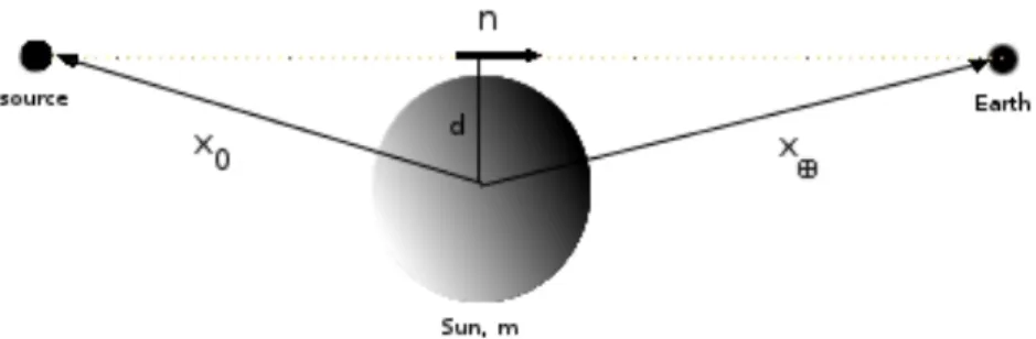
Cassini Bound onγ The strictest bounds onγhave been achieved using the Cassini spacecraft,
measuring the Doppler shift in a radio wave sent from the spacecraft to Earth on its way to Saturn.
This shift is influenced by the gravitational field of a massive object that the wave passes by, in this
case the Sun.
Writing the coordinate of a photon traveling in the direction ˆn as xj = ˆnj(t−t
0) +xjp, the
un-deflected part of the path is accounted for by the first term, and the term xj
p accounts for the
deflection. We take the vector ˆnto be normalized, ˆn·nˆ = 1.
Inserting the expression forxj into the geodesic equation for the general PPN metric, as in [20],
we get the equations for the deviationxp
d2xp
dt2 = (1 +γ) [∇U−2ˆn(ˆn· ∇U)] (2.3.7)
ˆ
n·dxp
dt = −(1 +γ)U (2.3.8)
Now, we can define the perturbation components parallel and perpendicular to the unperturbed
trajectory as
xp(t)k = nˆ·xp(t) (2.3.9)
xp(t)⊥ = xp(t)−nˆ[ˆn·xp(t)]. (2.3.10)
Then, with these definitions, equation (2.3.8) yields
dxpk
dt =−(1 +γ)U, (2.3.11)
where for a spherical source, the Newtonian potential is just U = m/r. Evaluating it along the
particle trajectory givesU =m/r(t), wherer(t) =|x0+ ˆn(t−t0) describes the path of the particle
originating at coordinates (t0,x0) and traveling at unit velocity in the ˆn direction. Using this
expression for the Newtonian potential, we can integrate equation (2.3.11) to get the the perturbation
to the path length parallel to the particle trajectory,
xp(t)k=−(1 +γ)m ln
r(t) +x(t)·nˆ
r0+x0·nˆ
. (2.3.12)
Now, we can use this expression to find the time difference for a particle to propagate in the
perturbed vs. the un-perturbed space-time. Writing the photon trajectory asx(t) =x0+ ˆn(t−t0) +
xp(t), we can dot both sides by the un-perturbed trajectory’s unit vector, and rearrange to get
t−t0 = |x−x0| −nˆ·xp(t) (2.3.13)
= |x−x0|+ (1 +γ)m ln
r(t) +x(t)·nˆ
r0+x0·nˆ
, (2.3.14)
Figure 2.1: Our coordinate system is centered at the Sun. A particle on an un-perturbed trajectory travels along the dashed line.
spacecraft is on the far side of the Sun from Earth, see figure 2.3.2. In this case, to find the round trip
travel time, we add together the travel time for each direction. We’ll ignore the first term in equation
(2.3.14), and just consider the part due to the perturbations. Taking x0 = 0, the denominator of
the second term in (2.3.14) is just d. Then, for the trip from Earth the the spacecraft, we get
r(t) +x(t)·nˆ = r⊕ +x⊕ ·nˆ and re+xe·nˆ = d, the impact parameter. For the return trip,
r(t) +x(t)·nˆ =rp+xp·nˆ, where thepsubscript denotes the coordinates for the spacecraft relative
to the Sun. Again, re+xe·nˆ = d. Since we’re treating just the case where the spacecraft is
approximately on the opposite side of the Sun from the Earth, we can approximatex⊕·nˆ 'r⊕,
xp·nˆ' −rp, andd'solarradius.
Putting these approximations in place, the term in the time change equation (2.3.14) due to the
space perturbation effects becomes
δt= 2(1 +γ)mln
4r ⊕rp
d2
(2.3.15)
This is the formula used by Bertotti et al. [26] to derive the Doppler shift in the Cassini
experiment. In particular, they find, after converting from natural units and replacingd=b,
γgr=
dδt
dt =−2(1 +γ) Gm
c3b
db
dt (2.3.16)
for the frequency shift. Since the spacecraft is much farther from the Sun than the Earth is,
using the approximation that the change in impact parameter is approximately the Earth’s velocity,
db/dt'vearth, they findγgr= 6×10⁻¹⁰, implyingγ−1<2.3·10−5[26].
Any proposed theory of gravity should fit this tight constraint within the scale of the solar system.
Bounds on β The current best constraint on β comes from the measurements of the perihelion
shift of Mercury. In Newtonian physics, orbits in 2-body systems form an ellipse. In general, the
orbits point of closest approach, the perihelion, can have some angular velocity,ω.
One can calculate the perihelion shift from the 2-body equations of motion, as in Will [20].
We’ll consider two bodies of massesm1 and m2, with total massm=m1+m2 and reduced mass
µ = m1m2/m. The instantaneous eccentricity is e, semi-major axis is a, and semi-latus rectum
is p = a(1−e2). The result, assuming a conservative gravity theory (which removes other PPN
parameters), is a change of
∆ω=6πm
p
1
3(2 + 2γ−β) +J2
R2
2mp
(2.3.17)
per orbit. Here, J2 is the magnitude of the quadrupole moment of the Sun, defined by J2 =
(C−A)/msunR2. CandAare the moments of inertia about the symmetry axis and equatorial axis,
respectively. Ris the radius, andmsunthe solar mass.
Most of the perihelion shift is due to perturbations from other planets. Once this is accounted
for, the remaining perturbation should be given by inserting the astronomical values for the Sun
and Mercury into (2.3.17),
˙
ω= 42.95
00
c
1
3(2 + 2γ−β) + 3×10
−4
J
2
10−7
(2.3.18)
Figure 2.2: In Newtonian gravity, Mercury would follow an elliptical orbit around the Sun. In GR, the orbit can be described well by the parameters of an ellipse instantaneously, but the ellipse precesses. The change ∆θshown is the change in the perihelion in a time interval ∆t. This precession can be described by the angular velocityωgiven above.
2.4 Constraints from Pulsar Data
We will see in Chapter 3 that binary systems in scalar-tensor theories can emit dipole gravitational
radiation. Consequently, observed binary systems put constraints on this class of theories. Eardley
[28] showed that the dipole contribution to the change in the orbital period is proportional to the
square of the difference in the object’s sensitivities,S2= (s
1−s2)2. This difference is not appreciable
for neutron star binary systems (NS-NS systems) like the double-pulsar PSR J0737-3039 [29], and so
the dipole emission has little effect. The difference is significant with NS-white dwarf systems. Alsing
et. al [30] examined these types of systems (as well as constraints from Cassini and the Nordtvedt
effect) to give exclusion maps showing how suppressed the scalar should be (how large its mass must
be) given a particular Brans-Dicke parameter (ωBD) for the scalar-tensor theory to be allowed by
Pulsar observations. Observations of PSR J1141-6545 appear to just rule out ωBD = 0, but these
Chapter 3
Tensor-Scalar Gravity
In this section, I will review an important class of metric theories of gravity: tensor-scalar theories.
These theories belong to a simple class of extensions to gravity where modifications are described
by a scalar field, φ. By letting φ→1, all modifications to GR vanish. The general class of these
theories allows for multiple scalar fields, and provides a metric on the space of these fields. These
models have been used, for example, in multi-field inflation. They include the double-field inflation
model [31, 32, 33], and other multi-scalar inflationary models. Other more restricted cases typically
involve just one scalar field. In the Lagrangian, this field may or may not have a potential term
associated with it, and the coefficient of the kinetic term may or may not depend on the field. What
distinguishes these theories from other theories that involve scalar matter fields is that the scalar
field only enters into the matter part of the Lagrangian as a conformal factor for the metric. Thus,
the scalar field only interacts with matter through its coupling with the metric field. In the rest of
this section, I will go into some detail on the basic manipulations of these theories, and distinguish
between similar theories that can lead to some confusion. I will then start with the most general
case, when there are multiple scalar fields with potentials, and introduce successive simplifications.
This leads to the classic Brans-Dicke scalar-tensor theories. Throughout the following sections, I
will point out significant physical phenomena and relate them back to the motivation for my original
research.
It is common to perform conformal transformations to make equations in scalar-tensor theories
easier to work with. These transformations transform the metric ˜gµν →g∗µν =A
2(φ)˜g
µν from the
physical conformal frame, in which the theory is defined, into a different conformal frame. Here,
A2(φ) is a positive real function of φ. Note that this transformation is different from a general
coordinate transformation. The physics in these two different frames can be very different:
energy-momentum may or may not be conserved in either frame, and the gravitational constant may not
actually be constant. Once the equations are transformed into a different frame, the equations are
manipulated. Results in the the physical frame are finally obtained by transforming back to the
original frame simply by inverting the transformation.
frame is the one where the scalar field couples directly to the scalar curvature,
SJ =κ
Z
d4xp−˜g(φR˜−ω0 φg
µν∂
µφ∂νφ−V(φ) +Lm(ψ,g˜µν)) (3.0.1)
Transforming to a different frame via a conformal transformation ˜gµν =A(φ)g∗µν, and changing the
coordinates inφspace, we can arrive at the so-called Einstein frame. This frame gets its name from
the fact that the gravitational action is the same as that in general relativity,
SE=κ
Z
d4x√−g∗(R∗−1
2g µν
∗ ∂µφ∂νφ−V(φ) +Lm(ψ, A(φ)gµν∗ )). (3.0.2)
I will now outline this procedure, as presented in [25]. First, we find it convenient to change φ
coordinates to give us a canonical kinetic term. We make the changeφ= 81ωϕ2, and rewrite (3.0.1)
as
SJ=κ
Z
d4xp−g˜( 1 8ωϕ
2R˜−1
2g µν∂
µϕ∂νϕ−V(ϕ) +Lm(ψ,˜gµν)). (3.0.3)
Next, we will perform the conformal transformation. First, we define F(ϕ) = ϕ2. We focus on
the first term in the Lagrangian, L1 = 12
√
−gF˜ (ϕ) ˜R, and find the transformation that results in
˜
R entering into the Lagrangian as it does in GR. We now need some basic properties of conformal
transformations. For the transformation
˜
gµν →gµν∗ =A
2(ϕ)˜g
µν
, we get
gµν =A2g∗µν,
p
−˜g=A−4√−g∗
. Then, definingf = logAandfµ=∂µf (thisf is not the be confused with thef(R) from modified
gravity theories, which is equivalent to 1
2F(ϕ)), we find that
˜
R=A2(R∗+ 6∗f −6g∗µνfµfν)
. Applying these to the first term of the Lagrangian, we get
L1=
√ −g∗
1 2F(ϕ)A
−2(R
Now, our goal is to get the term containingR∗ to enter into the Lagrangian as it does in GR, like √
−g∗12R∗. To do this, we setF(ϕ)A
−2 = 1, which gives us our definition forA(ϕ), specifying the
conformal transformation we were looking for asgµν =ϕgµν
∗ .
We have the term we’re looking for now, but have to finish transforming the action. The second
term in (3.0.4) can be eliminated by integrating by parts, andfµ=12F
0
F∂µϕso (3.0.4) becomes
L1=
√ −g∗
1 2R∗−
3 4
F0
F
2
gµν∗ ∂µϕ∂νϕ
!
.
Finally, the kinetic term,−1 2˜g
µν∂
µϕ∂νϕ, is transformed into
− 1
2Fg
µν
∗ ∂µϕ∂νϕ.
Then, since the second term ofL1 is of the same form, we can combine terms to get
− 1
2ϕ2g
µν
∗ ∂µϕ∂νϕ.
The final result is then
SE=
Z
d4x√−g∗ 1
2R∗− 1 2ϕ2g
µν
∗ ∂µϕ∂νϕ+Lm
.
3.1 Tensor Multi-Scalar Theory
3.1.1 Action and Field Equations
The most general tensor-scalar theory is one with multiple scalar fields, and with a potential for
those fields. Allowing for coupling between the kinetic terms, we can write the action for this in the
Einstein frame as [24], following Damour’s notation,
Stot=Sg∗+Sϕ+Sm (3.1.1)
where
Sg∗ =
c4
4πG∗ Z d4x
c √
g∗ R∗
4 (3.1.2)
Sϕ =
c4
4πG∗ Z d4x
c √
g∗ 1
2g µν
∗ γab∂µϕa∂νϕb+V(ϕa)
(3.1.3)
Sm = Sm
ψm, A2(ϕa)g∗µν
(3.1.4)
We’ve written this in terms of a metric, g∗µν, called the Einstein metric. This is not the metric
whose curvature is “felt” by matter. That metric is the one that enters into the matter action, as
indicated in the definition ofSm, and we write it ˜gµν =A2(ϕa)g∗µν.
We now should look into what physical effects this generalization has. We are concerned, in
particular, with how the radiation in this theory differs from general relativity.
3.1.2 Radiation Sources
In General Relativity, we can choose to examine perturbations to the Minkowski metric, ηµν,
and write our metric asgµν =ηµν+hµν in terms of the perturbation,hµν. If we keep only terms in
the Einstein equations linear in the perturbation, we will arrive at a wave equation for the metric
perturbations. We will detail this procedure in section 5.3.1. We will find the dominant contribution
to radiation to result from the second time derivative of the mass-quadrupole-moment of our source
mass distribution.
It helps to look at a particular case. We’ll examine two compact bodies orbiting each other with
circular orbits. See the figure to clarify the coordinate system. They will have masses m1 andm2,
total inertial massM =m(0)A +m(0)B , and ν=m(0)A m(0)B /M2. Their coordinates will bez
A andzB,
orbital radiusR =kZk =kzA−zBk, separation unit vectorN=Z/R, and their relative velocity
V=dZ/dt. We can write the dominant term for power radiated in GR as
PquadrupoleGR = 8G∗ 15c5
G
ABM2ν
R2
2
12V2−11(N·V)2
+O
1
c7
(3.1.5)
We can contrast this to the situation when scalar fields are introduced. In this case, we can have
scalar wave radiation. We find this to be sourced in a multipole expansion by as low as the monopole
Figure 3.1: Our coordinates are in the center-of-mass frame for the two-body system.
the portion radiated via the scalar field, given by the expressions
PmonopoleT M S =
G∗ c5
GABM2ν
R2
2
(N·V)2
5 3(α
a
A+αaB) (3.1.6)
−2
3(α a
AXA+αBaXB) +
βAba αbB+βBba αbA
1 +αAαB
2
+O(1
c7)
PdipoleT M S = G∗ 3c3
G
ABM2ν
R2
2
[αaA−αaB]2+O(1
c5) (3.1.7)
PquadrupoleT M S =
G∗
30c5
GABM2ν
R2
2
32V2−88
3 (N·V)
2
(3.1.8)
×[(αaA+αaB)−(αaAXA+αaBXB)]
2
+O
1
c7
(3.1.9)
and matches the GR expression for the portion radiated, at quadrupole order, via the
transverse-traceless metric perturbations. Here, αa
A =∂ln(mA(ϕ))/∂ϕa, and is a property of Ath body, and
βA
ab(ϕ) = DaDbln(mA(ϕ)), where Da is the covariant derivative with respect to the sigma model
metric,γab, andXA=m
(0)
A /M.
In general relativity, there is no source for monopole or dipole radiation. Conservation of mass
implies that there is no time-varying monopole moment for the mass distribution of a localized
source. Conservation of momentum implies the same for a time-varying mass dipole moment. The
existence of the former would imply the total mass-energy of a closed system were changing with
time. The latter would imply that the center of mass of a closed system were oscillating, which can’t
happen without external forces. This is why gravitational radiation in GR is due to a time-varying
quadrupole (and higher) moment.
In TMS theory, however, the source for radiation can be from the scalar field mass-energy. A
single body that is increasing in density can have increasing scalar field energy-momentum. Two
bodies orbiting each other with the same total energy, but different contributions to that
mass-energy from the scalar field will have a time-varying scalar field mass-energy-momentum dipole moment.
Thus, in TMS theory, we can have monopole and dipole radiation.
We notice, then, that in TMS theory we can have much greater total power radiation. The
quadrupole radiation in both TMS and GR are suppressed relative to the TMS dipole term by a
factor of order (v/c)2. This makes scalar radiation a potentially interesting way of investigating
TMS theory relative to GR.
Note that the dipole radiation vanishes for bodies with identical sensitivities, αa
i. Eardley [28]
points out that black holes always have sensitivity of unity. Dwarfs and normal stars have negligible
sensitivities of around 10−3and 10−6, respectively, and neutron stars have sensitivities ranging from
around 0.01 for 0.132M stars to 0.78 for 1.41M stars. Thus, systems with a star and black hole
would make the best candidates for strong dipole radiation.
3.2 Tensor-Scalar Theory: Brans-Dicke with Potential and Variableω
If we simplify Tensor-Multi-Scalar theory by allowing only one scalar field, we get the action for
a Brans-Dicke theory with potential and variableω. Restricting to one scalar, we drop the indices
on the sigma model metric,γab, and rewrite it asγ=γ(ϕ). We redefine theϕfield, and perform a
conformal transformation to the Jordan frame, and thus put the action in the form
S=
Z
d4x√−g
ϕR−ω(ϕ)
ϕ g
µνϕ
,µϕ,ν−V(ϕ) +Lm
. (3.2.1)
Varying the action gives the equations of motion
Gµν = −
4πG˜
ϕ T
(m)
µν +
ω(ϕ)
ϕ2
ϕ,µϕ,ν− 1 2gµνg
αβϕ ,αϕ,β
(3.2.2)
+1
ϕ(ϕ;µν−gµνϕ) +
1
2ϕgµνV(ϕ)
ϕ = 1
2ω(ϕ) + 3
−4πGT˜ (m)+ 2V(ϕ) +ϕV0(ϕ) +dω(ϕ)
dϕ g
µν
ϕ,µϕ,ν
(3.2.3)
physical effects are easiest to see. We’ll use this to examine a few effects in these generalized
Brans-Dicke theories.
3.2.1 Variation of Newton’s Constant
One effect that results from the scalar field coupling to the Ricci curvature in the Jordan frame
action is an effective variation of the gravitational constant,G, withϕ. As ϕcan vary throughout
space and time, so also can the effective gravitational constant. This is apparent when we look at
equation (3.2.2), and we see the place ofGin the GR Einstein equations taken byG/ϕ.
If the cosmological value of ϕ changes with time, we can have a slow time-variation of the
gravitational constant. The Viking Project [34] and binary pulsar data [35] constrain ˙G/G <
(0.2±0.4)×10−11years−1 and ˙G/G <(−0.06±0.2)×10−11years−1, respectively [25].
It should be noted that in the Einstein frame, the lack of coupling to the scalar curvature results
in the gravitational constant being constant [25].
3.2.2 Effect of Potential
If we restrict to the asymptotic region, where the scalar field takes its constant cosmological
value, the effect of including a potential term for the scalar field becomes more clear. Equation
(3.2.2) reduces to
Gµν = −
4πG˜
ϕ T
(m)
µν + 1
2ϕgµνV(ϕ), (3.2.4)
and so we have an effective cosmological constant term.
Another effect of including the potential is that the field has only a finite range.
3.3 Brans-Dicke without Potential with Constant ω
The least general class of TMS theories we’ll look at is one with one scalar field, no scalar
potential, and fixedω. This is of theoretical interest as a toy theory, and can be used to investigate
the effects of the non-minimal coupling term, √−gϕR, in the Lagrangian. This theory reduces to
GR in the limitω→ ∞. It can be shown that the presence of a non-minimal coupling term with no
ϕfield in the matter Lagrangian implies that the weak equivalence principle is obeyed [25].
Brans-Dicke theories imply immediate physical results involving an extra gravitational scalar
force. This would imply measurements for PPN parameters that differ from GR. In particular,
γ = 1+2+ωω, while β = 1 agrees with its value in GR. The parameterγ only agrees exactly with the
value in GR ifω→ ∞.
3.4 The Chameleon Mechanism
Brans-Dicke theories, for small enough ω, disagree with solar system experiments. Solar system
experiments impose the constraint ω > 40000 [36]. The generalized versions with potential can
get around this constraint through non-linear effects that suppress the scalar field’s effects at solar
system scales, but still allow it to act at larger scales. This is known as the chameleon mechanism.
We will follow the work of Khoury and Weltman, [37], in presenting this theory. We start with
the basic action in the Einstein frame,
S=
Z
d4x√−g∗ M2
P L 2 R
∗−1
2∂µφ∂ µφ
−V(φ)
+Smatter(ψ, e2βφ/MP Lgµν∗ ), (3.4.1)
where Einstein frame quantities are denoted with a∗.
To have a long-range, massless field in environments with no matter present, we require a
po-tential of the runaway form with no minimum. It should satisfy the constraints
lim
φ→∞V = 0 φlim→∞ V,φ
V = 0 φlim→∞ V,φφ
V,φ
= 0 (3.4.2)
and
lim
φ→0V =∞ φlim→0
V,φ
V =∞ φlim→0
V,φφ
V,φ
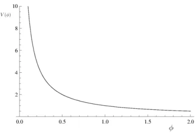
=∞, (3.4.3)
like and inverse power law potential,V(φ) =M4+nφ−n, for some mass scaleM and positive constant
n. A schematic functionV(φ) is pictured in figure 3.4
If we were to add to this a monotonically increasing function, we could introduce a minimum and
thus cause the potential to pick up a mass. We will now see that the field does indeed experience
an effective potential of this form in the Einstein frame. This is depicted in figure 3.4
The equation of motion for φresulting from the action (3.4.1) is
∇2φ=V
,φ−
β MP L
e4βφ/MP L˜gµνT˜
µν, (3.4.4)
Figure 3.2: This is a schematicV(φ) satisfying all the constraints in equations 3.4.2 to 3.4.3
Figure 3.3: This is a schematic potential V(φ) together with the exponential term, resulting in an effective potential with a minimum atφmin, even though the original potential was monotonically decreasing.
Minkowski space, we approximate gµν ≈ ηµν, and so ˜gµνT˜µν ≈ −ρ˜, where ˜ρ is the Jordan frame
energy density. Following [37], we express this in terms of the Einstein frame conserved energy
density,ρ= ˜ρe3βφ/MP L as
∇2φ=V
,φ+
β MP L
ρeβφ/MP L, (3.4.5)
and so we see that φ is governed by an effective potential of the type described above, Vef f =
V(φ) +ρeβφ/MP L. The value assumed by φat the minimum of the effective potential can be found
from
V,φmin+
β MP L
ρeβφmin/MP L = 0 (3.4.6)
and, if we interpret the field as a particle in a quadratic well, the mass of fluctuations about this
minimum is
m2min=V,φφ(φmin) + β
2
M2
P L
ρeβφmin/MP L, (3.4.7)
implying that the mass increases with local matter density. The presence of this effective mass
limits the range of the force associated with the scalar field, and so scalar forces are suppressed by
a Yukawa-like factor1,e−mminr/r.
As shown in [38], there is also a non-linear shielding effect in the Jordan frame. For an object
with an inertial massM, the effective gravitational mass becomesMef f =M1+2α
2
1+2α2. In effect, the
gravitational mass is smaller than the inertial mass due to a screening effect. This screening effect
operates when the gravitational well of an object, with mass M and characteristic size rc, is large
compared with the background scalar field,ϕ0. It is parameterized by'ϕ2α0
GM rc
−1
[38]. Here,α
is a parameter that comes from producing the Jordan frame equations by a conformal transformation
from the Einstein frame equations, using the conformal factorA2(ϕ) = 1−2αϕ, and following the
reverse of the procedure outlined at the beginning of Chapter 2. See figures 3.4,3.4
for an illustration of how this effect looks schematically in terms of the scalar field, given some
mass distribution. Note that the scalar generally tries to approach a constant value in a constant
background, but can’t when the backgrounds gravitational well is not deep enough.
There is a related perspective on the scalar interaction between objects that are large compared
to the range of the scalar field in their interiors. Consider a sphere of radiusR and energy density
ρin a vacuum. If the range of the scalar field is small inside the sphere, and large in the vacuum
outside of it, it’s range must interpolate between the two in a thin shell near the surface of the sphere.
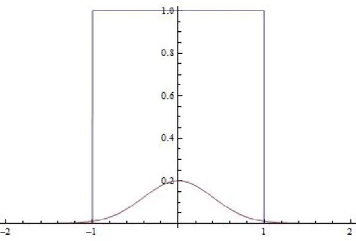
Figure 3.4: Here, the matter distribution (square curve) is plotted against distance along the central axis through a body in space. The gravity well of this body is weak, so elicits only a weak response (qualitatively depicted) from the scalar field, whose value relative,φ−φ0, to its background value
is depicted in the figure.
Figure 3.5: Here, the matter distribution (square curve) is plotted against distance along the central axis through a body in space. The gravity well of this body is rather strong, so elicits only a strong response (qualitatively depicted) from the scalar field, whose value relative,φ−φ0, to its background
value is depicted in the figure.
Khoury and Weltman show this analytically, and argue that this results in theφ-force between the
two objects being sourced only by a thin shell of material near their surfaces. This allows planetary
systems, with long rangeφ-forces between objects, to still pass solar system tests of gravity. Such a
thin shell is qualitatively depicted in the transitional area in figure 3.4 where the field interpolates
between its background value, and its value inside the matter distribution. Presumably, the value
inside the matter distribution is such thatmef f(φinside) is large compared its value at the external
Chapter 4
f(R)Gravity
4.1 Basic Theory
The action for general relativity is the Einstein-Hilbert action,
SEH =
Z
d4x√−gR+Smat(ψ, gµν), (4.1.1)
wheregµν is the space-time metric, g is its determinant,Ris its scalar curvature, and Smatt is the
matter action. The fieldψrepresents all matter fields of the theory.
From general relativity, we know that we can vary this action with respect togµν to produce the
Einstein field equations. We also know that there are two equivalent approaches to doing this: the
Einstein-Hilbert variational principle, or the Palatini variational principle. In the first case, the scalar
curvature,R, is the curvature defined by the metric connection, Γα µν= 12g
ασ(∂
µgσν+∂νgσµ−∂σgµν).
Varying the action with respect to the metric results in a term involvingδΓρ
µν 6= 0, resulting from
varying the connection with respect to the metric. In the second case, the scalar curvature is defined
by a connection,Γα
µν, that is independent of the metric. This is considered a field in its own right, and
need not have a physically interpretable metric associated with it. In this case, the scalar curvature
produced using this connection is usually denotedR, to distinguish it from the scalar curvature,R,
produced using the metric’s connection. This produces another set of field equations by variation
with respect to the independent field Γαµν. Combining all these equations givesR =R, and yields
the Einstein field equations. When generalizing the action, we will see that these two approaches
are not equivalent.
The basic action off(R) gravity is
S=
Z
d4x√−gf(R) +Smat(ψ, gµν), (4.1.2)
where Smat is the matter action, ψ are the matter fields, and gµν is the space-time metric. The
definition of the Jordan frame was made for scalar-tensor theories. It does not carry over directly
that the modification to the Einstein-Hilbert action made above introduces, in many cases, a scalar
degree of freedom. Other degrees of freedom could be introduced, but they turn out to introduce
instabilities. We will go more into this later. The action given in (4.1.2) turns out to be the most
general action we can use. This is why I chose to work withf(R) gravity theories.
With thef(R) gravity action, the two variational principles from GR are no longer equivalent.
The Einstein-Hilbert variational principle produces a theory called “metricf(R) gravity,”, and the
Palatini variational principle produces “Palatini f(R) gravity”. Palatini f(R) gravity is not
well-behaved, while metric f(R) gravity works well for certainf(R). We will now briefly go into some
detail about the problems with Palatini f(R) gravity, and then describe the constraints on f(R)
required by metricf(R) gravity. In these sections, we will generally follow the review by Sotiriou,
[8].
4.2 Problems with Palatini
There are several problems with Palatini f(R) gravity, which we will now illustrate. After
satisfying ourselves that Palatinif(R) gravity is not viable, we will restrict further consideration to
only metricf(R) gravity.
4.2.1 Metric algebraically related to energy-momentum
It has been shown that in Palatinif(R) gravity, the Ricci curvature is related algebraically, and
not differentially, to the matter distribution. We start from the field equations,
f0(R)R(µν)−
1
2f(R)gµν = κTµν, (4.2.1) ¯
∇λ(
√
−gf0(R)gµν) = 0, (4.2.2)
whereRis the Ricci curvature of the independent connection,gµν is the space-time metric, the bar
indicates covariant differentiation with respect to the independent connection, and (µν) indicates
symmetrization overµandν.
We can take the trace of (4.2.1) to get
f0(R)R −2f(R) =κT. (4.2.3)
relationship between the curvature and the matter. As Sotiriou suggests [8], this is undesirable
behavior. Consider the curvature sourced by a point particle, represented as a delta function. There
is extremely large curvature, even with very little mass. Consider also a discontinuity in the matter
distribution, like at the surface of a planet. This would introduce a discontinuity in the curvature.
While it is not a nice property, GR has this characteristic as well. In GR, by taking the trace of
the field equations, we getRis proportional toT. While it is nice to avoid this, it isn’t a fatal flaw.
4.2.2 Background-dependent Newtonian Limit
One can also show that when f00(R) 6= 0, the Newtonian limit of the metric depends on the
background. The solution for the first post-Newtonian correction to the 0-0 component of the
metric, for example, is [8]
h(1)00(t, x) = 2Gef fM
r +
V0
gφ0
r2+ Ω(T), (4.2.4)
where M = φ0
R
d3x0ρ(t, x0)/φ, φ is the gravitational scalar field, φ
0 is the value of the scalar
field far from any sources, Gef f is an effective gravitational constant, ρ is the energy density of
the source, V0 is the scalar potential evaluated at φ0, and Ω(T) = log(φ/φ0). While for some
background densities this will produce a Newtonian limit with γ = 1, it is impossible for the full
range of densities. Also, we again have the same problem of divergences and discontinuities in the
metric in response to delta-function or discontinuous sources that we did with the scalar curvature.
Consider what this means for the Newtonian force at the boundary of a planet!
The problems with Palatini f(R) gravity are severe enough that we will not consider those
theories any farther. We will instead turn consideration toward metricf(R) gravity.
4.3 Properties of Metric f(R) Gravity
Metric f(R) gravity uses the action (4.1.2) where R is the metric’s Ricci curvature, and the
Einstein-Hilbert variational principle is used. This produces the field equations
f0(R)Rµν− 1
2f(R)gµν −[∇µ∇ν−gµν]f
0(R) = κT
µν. (4.3.1)
Taking the trace of this equation yields
f0(R)R−2f(R) + 3f0(R) =κT, (4.3.2)
whereT is the trace of the matter energy-momentum tensor. With this, we can now consider what
the vacuum solutions of metric f(R) gravity look like. We will look for a maximally symmetric
space-time, and requireR=C for some constantC. The field equations (4.3.1) reduce to
f0(C)Rµν− 1
2f(C)gµν= 0, (4.3.3)
which gives Rµν = gµνC/4, which is de Sitter or anti-de Sitter, depending on if C is positive or
negative. Later, when we expand the metric in a series, we will treat our vacuum solution for the
metric as approximately Minkowskian. It will be understood that we are taking appropriate time
and distance scales for this to be a reasonable approximation. These will be, as in GR, much less
than the Hubble time and Hubble radius.
Note that we can turn equation (4.3.1) into a much more familiar form. By using the Einstein
tensorGµν =Rµν−12gµνR, we can rewrite (4.3.1) as
Gµν =
κ f0Tµν+
1
2f0(f −Rf 0)g
µν+ 1
f0[∇µ∇ν−gµν]f 0.
Now compare this with the field equations for Jordan frame scalar-tensor gravity, equations (4.3.4),
which I’ll re-write here for convenience,
Gµν = −
4πG˜
ϕ T
(m)
µν +
ω(ϕ)
ϕ2
ϕ,µϕ,ν− 1 2gµνg
αβϕ ,αϕ,β
(4.3.4)
+1
ϕ(ϕ;µν−gµνϕ) +
1
2ϕgµνV(ϕ)
ϕ = 1
2ω(ϕ) + 3
−4πGT˜ (m)+ 2V(ϕ) +ϕV0(ϕ) +dω(ϕ)
dϕ g
µνϕ ,µϕ,ν
. (4.3.5)
By taking ω(ϕ) = 0, V(ϕ) = f −Rf0, andϕ = f0(R), we see that we’re left with the equations
for metricf(R) gravity, equations (4.3.1). This is equivalent to an ω= 0 Brans-Dicke theory with
potential. To produce this from an action, however, we need that f00(R)6= 0. We will now go into
some detail on this point.
4.3.1 Equivalence of f(R)and Scalar-Tensor Gravity
There is an equivalence, under appropriate circumstances, between metric and Palatini f(R)
gravity and a Brans-Dicke theory with potential. We will now show this equivalence, so we can
We take the standard approach [8] and start with the metricf(R) action, (4.1.2), and introduce
an auxiliary fieldχ. We produce the dynamically equivalent action,
Smet= 1 2κ
Z
d4x√−g[f(χ) +f0(χ)(R−χ)] +Sm(gµν, ψ). (4.3.6)
If we vary with respect toχ, we get
f00(χ)(R−χ) = 0. (4.3.7)
This implies, as long asf00(R)6= 0, thatR =χ. This reproduces the metric f(R) action. This is
where the equivalence breaks down whenf00(R)6= 0. Now, to put this in the form of a Brans-Dicke
theory, we make some redefinitions. We define φ=f0(χ), and V(φ) =χ(φ)φ−f(χ(φ)). Then, the
action (4.3.6) becomes
Smet= 1 2κ
Z
d4x√−g[φR−V(φ)] +Sm(gµν, ψ). (4.3.8)
This is the action for a Brans-Dicke theory with potential with Brans-Dicke parameterω0= 0. This
is the Jordan frame for the tensor-scalar theory equivalent to metric f(R) gravity for f00(R)6= 0.
The field equations for this theory, after some manipulation, are
Gµν=
κ φTµν−
1
2φgµνV(φ) +
1
φ(∇µ∇νφ−gµνφ), (4.3.9)
and
3φ+ 2V(φ)−φV0(φ) =κT. (4.3.10)
We will see later that the condition f00(R) → 0 causes the scalar mass to diverge. Another
viewpoint is that it causes the coefficient of the kinetic term in (4.3.10) to be 0 for small perturbations
toR, so the scalar perturbations have no dynamics.
It will be useful to have this in the Einstein frame as well. That can be achieved by the conformal
transformation to the metric ˜gµν, defined by ˜gµν =φgµν, along with the scalar field redefinition,
φ=f0(R) =e √
2κ
3φ˜. (4.3.11)
Then, the action (4.3.8) transforms to
Smet=
Z
d4xp−g˜
"
˜
R
2κ−
1 2∂
αφ∂˜
αφ˜−U(φ)
#
+Sm(e− √
2κ
3φ˜˜gµν, ψ), (4.3.12)
where
U( ˜φ) =Rf
0(R)−f(R)
2κ(f0(R))2 , (4.3.13)
andR=R( ˜φ). This form of the action will be useful for analyzing in the context of the chameleon
mechanism.
4.3.2 Chameleon Mechanism inf(R) Gravity
Sortiriou [8] shows that metricf(R) gravity fails to satisfy experimental constraints on the
post-Newtonian parameter γ unless the effects of the scalar field are suppressed on solar system scales.
The most interesting suppression, in the sense that there are still scalar field effects on large scales,
is via the chameleon mechanism. As detailed in section 3.4, the chameleon mechanism requires the
potential in the Einstein frame to satisfy the constraints (3.4.2) and (3.4.3). In the context of the
previous section, the potential (4.3.13) should satisfy these same constraints. This translates to
fairly complicated constraints on the form off(R).
There has been some work on theories satisfying these constraints, and they have been dubbed
“vanillaf(R) gravity”, since they are observationally indistinguishable from GR with a cosmological
constant.
Instead of taking this approach, I will ask what a theory might look like if f00(R)6= 0 in certain
environments. We can consider several cases of interest. First, if f00(R) 6= 0 in sufficiently dense
environments, and f00(R) = 0 elsewhere. Second, wheref00(R) = 0 in dense environments, and is
non-zero elsewhere, and third, where f00(R) = 0 for some particular value of R, and is non-zero
elsewhere. The PPN parameter was derived under the condition that f00(R) 6= 0. As long as
f00(R) = 0 at solar system scales, we should satisfy solar system constraints on γ. If f00(R) = 0
for some particular R, we expect that we would need the chameleon mechanism to be effective for
typicalRin our solar system.
4.3.3 Theoretical Constraints
We have talked a little about the theoretical constraints on scalar field theories. Of course, if