NON-PARAMETRIC MACHINE LEARNING METHODS FOR CLUSTERING
AND VARIABLE SELECTION
Qian Liu
A dissertation submitted to the faculty at the University of North Carolina at Chapel
Hill in partial fulfillment of the requirements for the degree of Doctor of Philosophy in
the Department of Biostatistics.
Chapel Hill
2014
Approved by:
Eric Bair
Michael Kosorok
Andrew Nobel
Gary Slade
c
2014
Qian Liu
ABSTRACT
Qian Liu: Non-parametric machine learning methods for clustering and variable
selection
(Under the direction of Eric Bair)
Non-parametric machine learning methods have been popular and widely used in
many scientific research areas, especially when dealing with high-dimension low sample
size (HDLSS) data. In particular, clustering and biclustering approaches can serve as
exploratory analysis tools to uncover informative data structures, and random forest
models have their advantage in coping with complex variable interactions.
In many situations it is desirable to identify clusters that differ with respect to
only a subset of features.
Such clusters may represent homogeneous subgroups of
patients with a disease. In this dissertation, we first propose a general framework
for biclustering based on the sparse clustering method. Specifically, we develop an
algorithm for identifying features that belong to biclusters. This framework can be
used to identify biclusters that differ with respect to the means of the features, the
variances of the features, or more general differences. We apply these methods to
several simulated and real-world data sets, and the results of our methods compare
favourably with previous published methods, with respect to both predictive accuracy
and computing time.
As a follow up to the biclustering study, we further look into the sparse clustering
algorithm, and point out a few limitations of their proposed method for tuning
pa-rameter selection. We propose an alternative approach to select the tuning papa-rameter,
and to better identify features with positive weights. We compare our algorithm with
the results suggest that our method out-performs the existing method, especially in
presence of weak clustering signal.
For the last project, we consider random forest variable importance (VIMP) scores.
We propose an alternative algorithm to calculate the conditional VIMP scores. We
test our proposed algorithm on both simulated and real-world data sets, and the results
suggested that our conditional VIMP scores could better reveal the association between
predictor variables and the modelling outcome, despite the correlation among predictor
I would like to dedicate this Doctoral dissertation to my one year old daughter,
Emmalyn Pu, who came like an angel and brightened up my life. I wish all the best
for her.
And with this opportunity, I would like to address a special thank you to my dear
husband, Dongqiuye Pu. We met in college when we were both young and full of dreams.
Now we have been holding hands and sharing 10 years of wonderful life together. With
laughter and tears, we grow as a family. I hope we can continue this sweet journey for
Acknowledgments
I would like to first acknowledge the inspirational instruction of Dr. Eric Bair, who
is the best advisor I can ever wish for, and also a good supporting friend outside the
scope of biostatistics.
I would also like to acknowledge my fantastic committee members, Drs. Michael
Kosorok, Andrew Nobel, Gary Slade, and Donglin Zeng. They have been super nice
and helpful, both on my research and on my career development.
Last but not the least, I would like to acknowledge my friends and family. I can not
go this far without your generous support and love. I am blessed to have you in my
Table of Contents
List of Tables
. . . .
x
List of Figures
. . . .
xi
1
Literature Review
. . . .
1
1.1
Clustering and biclustering . . . .
1
1.1.1
An overview of competing biclustering approaches . . . .
3
1.1.2
Sparse clustering and GAP statistic . . . .
8
1.2
Random forests and VIMP . . . .
11
1.2.1
Trees and random forests . . . .
11
1.2.2
VIMP: reference for variable selection . . . .
13
1.2.3
Conditional VIMP scores . . . .
14
1.2.4
Review on VIMP statistical test and variable selection
. . . . .
15
2
Biclustering via sparse clustering
. . . .
17
2.1
Introduction . . . .
17
2.2
Methods . . . .
18
2.2.1
Sparse Clustering . . . .
18
2.2.2
Biclustering Via Sparse Clustering
. . . .
20
2.2.3
Estimating the Null Distribution of the Weights . . . .
23
2.2.5
Existing Biclustering Methods . . . .
27
2.2.6
Evaluating the Reproducibility of Biclusters . . . .
28
2.2.7
Computational Details . . . .
29
2.3
Results . . . .
30
2.3.1
Simulation Studies . . . .
30
2.3.2
Analysis of OPPERA data . . . .
36
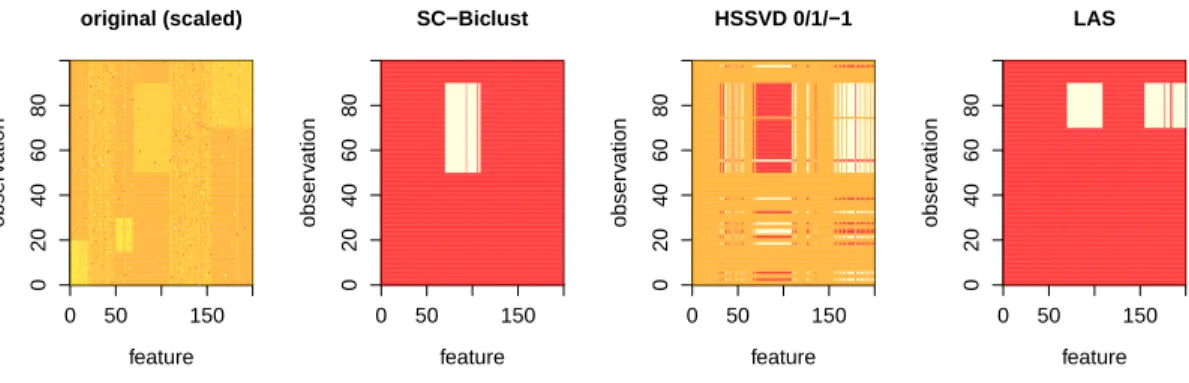
2.3.3
Analysis of a breast cancer gene expression dataset . . . .
38
2.3.4
Analysis of methylation data . . . .
38
2.4
Discussion . . . .
39
3
Soft-thresholding sparse clustering
. . . .
59
3.1
Introduction . . . .
59
3.1.1
Sparse clustering . . . .
60
3.1.2
GAP statistic and tuning parameter selection . . . .
62
3.1.3
Simulation example of sparse clustering null distribution . . . .
63
3.2
ST-Spcl: soft-thresholding sparse clustering
. . . .
64
3.2.1
Iterative procedure of the ST-Spcl algorithm . . . .
65
3.2.2
Estimating the Null Distribution of the Weights . . . .
66
3.3
Simulation example to test the performance of ST-Spcl . . . .
68
3.4
Real data application on breast cancer gene expression. . . .
69
3.5
Discussion . . . .
70
4
Random forests variable importance
. . . .
79
4.1
Introduction . . . .
79
4.1.1
Breiman’s VIMP: reference for variable selection . . . .
80
4.1.2
Strobl’s VIMP: motivation and one possible solution
. . . .
82
4.2
Methods . . . .
84
4.2.1
An alternative approach to calculate conditional VIMP . . . . .
84
4.3
Simulation example of various VIMPs comparison . . . .
85
4.4
Real data application on OPPERA . . . .
87
4.5
Discussion . . . .
88
5
Conclusion
. . . .
93
List of Tables
2.1
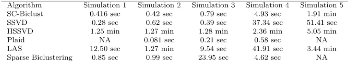
Comparison of computing times (average of 100 simulations) . . . .
49
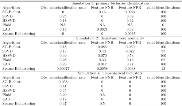
2.2
Comparison of prediction accuracy: simulations 1, 2, and 4 (average of
100 simulations) . . . .
50
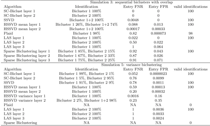
2.3
Comparison of prediction accuracy: simulations 3 and 5 (average of 100
simulations) . . . .
51
2.4
Comparison of reproducibility (average of 100 simulations
×
10 partitions) 52
2.5
Comparison of stopping rule: simulations 1 and 3 (average of 100
simu-lations) . . . .
53
2.6
OPPERA: comparison of different biclustering algorithms . . . .
54
2.7
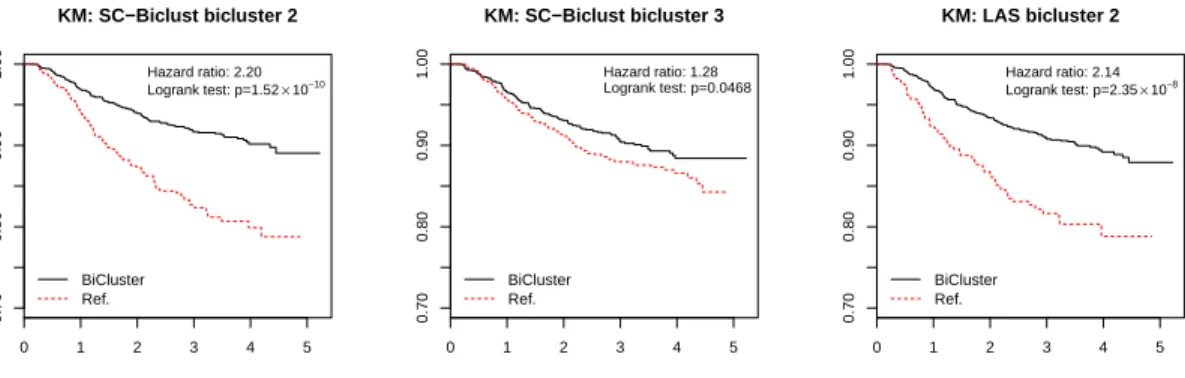
OPPERA: association between biclusters and chronic TMD . . . .
55
2.8
OPPERA: association between biclusters and first-onset TMD (logrank
test) . . . .
56
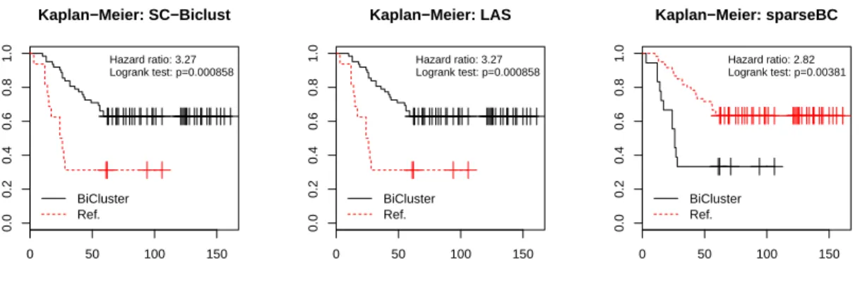
2.9
Gene expression: Comparison of biclustering and survival analysis results. 57
2.10 Methylation: association between biclusters and cancer . . . .
58
3.1
Sparse clustering comparison (average of 100 simulations) . . . .
77
3.2
Gene expression: Comparison of clustering and survival analysis results.
78
4.1
Simulation example: median VIMP across 100 simulations . . . .
91
List of Figures
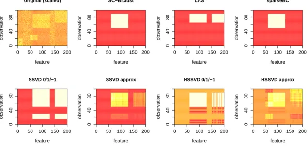
2.1
Simulation example: primary bicluster identification. . . .
42
2.2
Simulation example: departure from normality.
. . . .
43
2.3
Simulation example: sequential biclusters with overlap. . . .
44
2.4
Simulation example: non-spherical biclusters. . . .
45
2.5
Simulation example: variance biclustering. . . .
46
2.6
OPPERA Kaplan-Meier plots. . . .
47
2.7
Breast cancer gene expression Kaplan-Meier plot. . . .
48
3.1
Simulation example of sparse clustering null distribution. . . .
72
3.2
Simulation example of feature weights from permuted sparse clustering
null data.
. . . .
73
3.3
Simulation example of sparse clustering null data: ST-Spcl vs. sparse
clustering. . . .
74
3.4
Simulation example of bicluster with homogeneous mean: ST-Spcl vs.
sparse clustering. . . .
75
3.5
Breast cancer gene expression Kaplan-Meier plot. . . .
76
Chapter 1
Literature Review
1.1
Clustering and biclustering
Unsupervised exploratory methods play an important role in the analysis of
high-dimension low sample size (HDLSS) data, such as microarray gene expression data.
Such data sets can be expressed in the form of a
n
×
p
matrix
X
, where each row
corresponds to one observation and each column corresponds to one predictor variable.
In clustering and biclustering studies, we refer to observations as objects, and predictor
variables as features. Both terms will be used interchangeably in the following sections.
Unsupervised learning is a powerful tool for discovering interpretable structures
within HDLSS data without reference to external information. In particular, clustering
methods partition observations into subgroups based on their overall feature patterns.
In general, the observations are assigned into different sub-categories in such a way that
the objects within the same sub-category (called a cluster) are more similar to each
other than to those outside. And there is no single standard in determining the
sim-ilarity among observations – different clustering algorithms have different definitions,
depending on the study purpose and the data structure encountered. But clustering
methods in general will consider all the features when making the decision.
In many situations, these clusters may differ with respect to only a subset of the
Biclustering methods may be useful in situations where clusters are formed by only a
subset of the features. Biclustering aims to identify sub-matrices
U
within the original
data matrix
X
. The results may be visualized as two-dimensional signal blocks (after
reordering the rows and columns) containing only a subset of the observations and
a subset of the features. For example, in a gene expression data set collected from
cancer patients, there may exist a subset of genes whose expression levels differ among
patients with a more aggressive form of cancer. Identifying such a bicluster may aid in
the treatment of the cancer patients.
In general, biclustering results in rectangular signal blocks (called biclusters) where
the entries within are more similar to each other than to those outside. Different
bi-clustering algorithms have different definitions for this similarity measure, thus leading
to different biclusters of interest. Here we define biclusters as sub-matrices
U
of the
original data matrix
X
such that the observations within
U
are different from the
ob-servations not contained in
U
with respect to the features in
U
. In other words, the
choice of features influences which observations form the biclusters.
We can view clustering as a one-step partitioning method that partitions only the
set of observations. Biclustering, on the other hand, is a two-step partitioning method
that identifies partitions with respect to both features and observations. However, given
a set of features, the problem of biclustering reduces to the problem of partitioning the
observations with respect to this set of features, a problem which can be solved using
conventional clustering methods. Thus, one may identify biclusters by identifying the
features that define the biclusters and then clustering with respect to these features.
In recent years several methods have been proposed for identifying features that
de-fine such clusters. In the first part of the dissertation, we will show how the “sparse
clustering” method (29) may be used to identify biclusters under this framework. The
variances as well as more complex differences.
1.1.1
An overview of competing biclustering approaches
As the association between objects and features are defined variously, different
bi-clustering algorithms can lead to different results. One intuitive and commonly used
method is to independently cluster rows and columns through a multivariate clustering
method (9). This method can be further improved through simultaneous clustering,
which is also known as co-clustering (12). Or, one can rearrange the rows and columns
and search for rectangular blocks whose entries are on average large and positive (red)
or large and negative (green) (28). All these criteria make applicable sense, depending
on the specific data structures encountered. In this section, we briefly describe the
biclustering methods to which we will compare our algorithms in the first part of the
dissertation.
The Plaid method
Bicluster was first proposed in a way that the elements of a bicluster
U
should
be well fitted by a two-way ANOVA model (6). Based on that, the Plaid algorithm
was developed as an iterative procedure to approximate the data matrix
X
by a sum
of sub-matrices whose entries follow two-way ANOVA models (15). For a given n
×
p
data matrix, the Plaid model wants to achieve a small value of
1
2
n
X
i
=1
p
X
j
=1
(
Y
ij
−
θ
ij
0
−
K
X
k
=1
θ
ijk
ρ
jk
κ
ik
)
2
,
(1.1)
Here
Y
ij
denotes the
ij
th entry within the data matrix;
θ
ijk
denotes the response shared
j
is in the
k
th feature block and 0 otherwise; and
κ
ik
is 1 if object
i
is in the
k
th object
block and 0 otherwise.
Built on two-way ANOVA models, the Plaid algorithm treats objects and features
symmetrically, which is convenient and suitable for data structures where rows and
columns are interchangeable. Biclusters identified by the Plaid algorithm have entries
more similar to each other than to those outside, with respect to both objects and
features under the two-way ANOVA model setting. Multiple biclusters can be detected
by this method.
For the algorithm comparison in this biclustering study, the default setting of the
Plaid algorithm was used, and datasets were feature/column scaled before running
through the algorithm.
The Large Average Submatrix (LAS) method
As the data dimension increases, it is more difficult to analyse the data through
simple two-way ANOVA models; and treating objects and features symmetrically by
ignoring their natural relationship can be a waste of information in some situations.
The LAS algorithm was proposed by defining biclusters
U
as sub-matrices with the
averages of entries large and positive (red) or large and negative (green) (20) . The
algorithm is based on an additive model where the data matrix
X
can be expressed as
a sum of
K
constant sub-matrices with noise, as follows:
x
ij
=
K
X
k
=1
α
k
I
(
i
∈
A
k
, j
∈
B
k
) +
ε
ij
,
i
∈
[
m
]
, j
∈
[
n
]
,
(1.2)
where
A
k
⊆
[
m
] and
B
k
⊆
[
n
] are the row and column sets of the
k
th sub-matrix ([s]
denotes the set of integers from 1 to s),
α
k
∈
R
is the level of the
k
th sub-matrix, and
ε
ij
are independent
N
(0
,
1) random variables. When
K
= 0, the model reduces to the
to a significance based score function for sub-matrices/biclusters. Specifically, the score
assigned to a
k
×
l
sub-matrix
U
of
X
with average Avg(
U
)=
τ >
0 is defined by
S
(
U
) =
−
log
m
k
n
l
Φ(
−
τ
)
√
kl
.
(1.3)
The score function (1.3) can be viewed as a significance measure of departure from the
null model, which accounts for the size of the sub-matrix
U
and also the mean of the
entries within
U
.
LAS algorithm also treats objects and features symmetrically, but instead of
fit-ting two-way ANOVA models, the algorithm looks for signal blocks where the average
entries within are more close to each other than to those outside, with respect to the
numeric mean of the entries. The LAS algorithm has built in transformation functions
recommended for certain data structures, which is convenient and useful. LAS
algo-rithm is able to identify multiple biclusters within a given data set, and to output the
numeric mean and associated LAS score as a reference of the statistical significance for
each bicluster detected.
For the algorithm comparison in this biclustering study, default setting of the LAS
method was applied, including the default data transformation if recommended by the
method.
The Sparse singular value decomposition (SSVD) method
The SSVD method was developed as another alternative for biclustering, which
searched for a low-rank, checkerboard structured matrix approximation to the original
the first
K
≤
τ
rank-one matrices of
X
, in the form of
X
=
UDV
T
=
τ
X
k
=1
s
k
u
k
v
T
k
≈
X
(
k
)
≡
K
X
k
=1
s
k
u
k
v
T
k
,
(1.4)
where
τ
is the rank of
X
,
U
= (
u
1
, . . . , u
τ
) is a matrix of orthonormal left
sin-gular vectors,
V
= (
v
1
, . . . , v
τ
) is a matrix of orthonormal right singular vectors,
D
= diag(
s
1
, . . . , s
τ
) is a diagonal matrix with positive singular values
s
1
≥
. . .
≥
s
τ
on its diagonal.
With the adaptive lasso penalty, the minimizing objective for SSVD can be
ex-pressed as
||
X
−
s
uv
T
||
2
F
+
sλ
u
n
X
i
=1
w
1
,i
|
u
i
|
+
sλ
v
d
X
j
=1
w
2
,j
|
v
j
|
,
(1.5)
where
s
is a positive scalar,
u
is a unit
n
-vector,
v
is a unit
d
-vector, and
w
1
,i
’s and
w
2
,i
’s are data-driven weights, as explained in (30).
The sparsity-inducing penalties force the singular vectors to contain many zero
entries, with the non-zero entries corresponding to objects and features that form the
bicluster of interest. The SSVD method also treats objects and features symmetrically,
and searches for a checkerboard structured matrix to approximate the original data
matrix. The resulting approximation matrix has real value entries, with non-zero entries
correspond to the biclusters of interest.
In the algorithm comparisons in this biclustering study, default setting for the SSVD
method was applied. For result visualization on the figures, we transformed the
result-ing sresult-ingular vectors to be 0/
±
1 based on the signs of the entries. In prediction accuracy
and reproducibility comparisons, we further dichotomized the results into 0/1 as we only
Heterogeneous SSVD (HSSVD) method
Based on the framework of SSVD, another group developed the HSSVD method
to detect both mean and variance biclusters in the presence of unknown heterogeneous
residual variance (5). HSSVD defines biclusters as subsets of the data matrix with the
same mean and variance. It assumes a background layer where all the elements share
a common mean and variance, and all the biclusters have rectangular structures with
distinct mean or variance compared to the background layer. The HSSVD method
assumption can be expressed in the form of a random effect model as follows
X
=
Ξ
+
ρ
2
Σ
×
Φ
+
b
J
,
(1.6)
where
X
is the observed data,
Ξ
= (
ξ
ij
) is an
n
×
p
matrix representing the signal,
and
Φ
= (
φ
ij
) is an
n
×
p
matrix with i.i.d. random components with mean 0 and
variance 1. The heterogeneous variance signal is represented by this
n
×
p
matrix
Σ
= (
σ
ij
), with
ρ
, a finite positive number serving as a common scale factor.
J
n
×
p
is
an
n
×
p
matrix with all values equal to 1, and this finite number
b
serves as a common
location factor.
The HSSVD model makes the sparsity assumption that the majority of
ξ
ij
values
are 0 and the majority of
σ
ij
values are 1, and the mean structure
Ξ
and the variance
structure
Φ
are both low rank. Beyond the scope of the entry mean differences, the
HSSVD algorithm also studies the behavior of entry variances. It introduces a new
concept of biclusters with heterogeneous variances, which are commonly encountered
in some scientific research areas such as DNA methylation, where the methylation level
influences the variance of the measurements.
For algorithm comparisons in this biclustering study, default setting for the HSSVD
and
v
were transformed into 0/
±
1 for easier visualization in the figures, and further
dichotomized into 0/1 for prediction accuracy and reproducibility comparisons.
1.1.2
Sparse clustering and GAP statistic
Sparse clustering
The standard
k
-means clustering algorithm partitions a data set into
k
sub-categories by maximizing the between cluster sum of squares (BCSS). The BCSS is
calculated by taking the sum of the BCSS’s for each individual feature. This implies
that all the features are equally important. However, as we have discussed previously,
in many situations the clusters differ with respect to only a fraction of the features,
and these truly associated features do not necessarily contribute equally. In such
sit-uations, giving equal weights to all features when clustering may produce inaccurate
results. This is especially true for HDLSS problems, where the number of the features
is much bigger than the number of objects. To overcome this problem, the Tibshirani
group proposed a novel clustering method which they called “sparse clustering” (29).
Under sparse clustering where the original data matrix is with dimension
n
×
p
, each
feature is given a non-negative weight
w
j
, j
= 1
,
2
, . . . , p
, and the following weighted
version of the BCSS is maximized:
maximize
C
1,...,C
K,
w
(
p
X
j
=1
w
j
1
n
n
X
i
=1
n
X
i
0=1
d
i,i
0,j
−
K
X
k
=1
1
n
k
X
i,i
0∈
C
k
d
i,i
0,j
!)
subject to
||
w
||
2
≤
1
,
||
w
||
1
≤
s, w
j
≥
0
∀
j.
(1.7)
Here
X
ij
represents observation
i
for feature
j
of the data matrix
X
and
i
∈
C
k
if
and only if observation
i
belongs to cluster
k
.
d
i,i
0,j
is a distance metric between any
d
i,i
0,j
= (
X
ij
−
X
i
0j
)
2
. The
L
1
bound on
w
,
s
, is a tuning parameter, and can be
either pre-specified by the customer or selected through certain procedure, which we
will discuss in detail later.
They also describe an iterative procedure for maximizing (1.7) (29):
1. Initially let
w
1
=
w
2
=
. . . w
p
.
2. Maximize (1.7) with respect to
C
1
, C
2
, . . . , C
K
by applying the standard
k
-means
algorithm with the appropriate weights. In other words, apply the
k
-means
al-gorithm where the dissimilarity between observations
i
and
i
0
is defined to be
P
p
j
=1
w
j
d
i,i
0,j
.
3. Maximize (1.7) with respect to the
w
j
’s by letting
w
j
=
S
(
b
j
,
∆)
k
S
(
b
j
,
∆)
k
2
(1.8)
Here
b
j
is the (unweighted) between cluster sum of squares for feature
j
and
S
(
x, y
) = sign(
x
)(
|
x
| −
y
)
+
is a soft-threshold operator. ∆ is chosen so that
P
j
|
w
j
|
=
s
(∆ = 0 if
P
j
|
w
j
| ≤
s
). See (29) for the justification for (1.8).
4. Iterate steps 2 and 3 until the algorithm converges.
Note that (1.8) implies that as
s
increases, the number of nonzero
w
j
’s decreases. Thus,
for sufficiently small values of
s
, only a subset of the features contribute to the cluster
assignments, and the magnitude of
w
j
represents the contribution of feature
j
to the
clustering result. So, this method is useful in situations where the clusters differ with
respect to only a subset of the features. We can further imagine that in extreme cases,
when the tuning parameter
s
is selected properly and
K
= 2, we might be able to
based on these features, which leads to a bicluster with only a subset of observations
and a subset of features.
A variant of this procedure can be used to perform sparse hierarchical clustering as
well. In sparse hierarchical clustering, each feature is once again given a non-negative
weight and the cluster hierarchy is constructed using these weighted features. The value
of the weights again depends on a tuning parameter
s
, and some weights are forced to
0 when the tuning parameter is sufficiently small (29).
GAP statistic and tuning parameter selection
The GAP statistic was first proposed as a reference tool to select the optimal
number of clusters (26). They defined
W
k
as the pooled within-cluster sum of squares
around the cluster mean in the following manner:
W
k
=
k
X
r
=1
1
2
n
r
D
r
,
(1.9)
where
k
is the number of clusters,
n
r
is the number of observations within the
r
th
cluster, and
D
r
=
P
i,i
0∈
C
r
d
ii
0is the sum of the pairwise distances for all points in
cluster
r
. The GAP statistic is further defined as
GAP
n
(
k
) =
E
n
∗
log (
W
k
)
−
log (
W
k
)
,
(1.10)
where
E
n
∗
denotes the expect ion under a sample of size
n
from the reference distribution.
The sparse clustering method suggested the following algorithm to select the
tun-ing parameter
s
from a set of candidate values based on the GAP statistic through
independent observation permutation (29):
1. Obtain permuted data sets
X
1
, . . . , X
B
by independently permuting the
2. For each
s
, compute
O
(
s
) =
P
j
w
j
(
n
1
P
n
i
=1
P
n
i
0=1
d
i,i
0,j
−
P
K
k
=1
1
n
kP
i,i
0∈
C
k
d
i,i
0,j
)
as the objective obtained by performing sparse
K
-means clustering within tuning
parameter value
s
on the original data set
X
, and
O
b
(
s
) as the corresponding
objective for the permuted data set
X
b
. The GAP statistic for a given value of
s
is then calculated as
GAP
(
s
) = log (
O
(
s
))
−
1
B
P
B
b
=1
log (
O
b
(
s
)).
3. The optimal tuning parameter
s
∗
is chosen such that the corresponding
GAP
(
s
∗
)
is the largest.
Through this algorithm, they want the GAP statistic to measure the strength of the
clustering obtained on the real data relative to the clustering obtained on null data.
And their argument for the independent observation permutation is that even though
there may be strong correlation between the features in the original data set
X
, the
feature in the permuted data sets
X
1
, . . . , X
B
are uncorrelated with each other. And
this uncorrelated structure is desired as in their reference null distribution, all the
fea-tures should be uncorrelated and there should be no subgroups (e.g. clusters) on the
object dimension (29).
1.2
Random forests and VIMP
1.2.1
Trees and random forests
A decision tree is a tree-shape structure for modelling decisions and their possible
consequences. Each internal node on the tree represents a test or a decision rule of an
attribute, each branch represents a possible outcome of the test, and each leaf node
represents a class label, e.g. the decision taken after considering all attributes.
compared to parametric models when dealing with non-linear effects, arbitrary
inter-actions, and missing values. However, it also has one embedded drawback as the lack
of accuracy.
Random forests are a data mining method for classification that are based on
sim-ple decision trees (3), and can be used to evaluate the association between a response
variable and a large number of predictors. By constructing multiple decision trees on
randomly selected training sets and taking the average of the outputting class labels
from individual trees, random forests are more accurate and reliable than simple
deci-sion trees (3). In order to build a decideci-sion tree in random forests, a bootstrap sample is
first selected from the data, with the observations excluded from the bootstrap sample
known as the ”out of bag” (OOB) observations. A decision tree is then fit based on
this bootstrap sample, using only a subset of features on each node. Repeat the
pro-cess multiple times and take the average of the results, we will end up with a random
forest model. Since the randomly drawn bootstrap samples are diverse in nature, the
resulting decision trees are unstable, but their average result, e.g. the random forest
model, will produce a more stable and accurate prediction of the modelling outcome.
Specifically, the prediction accuracy was approved by smoothing the hard cut decision
boundaries due to the splitting in single decision trees, which also reduced the variance
of the prediction (4).
In high dimensional data setting, the VIMP scores have been suggested for
ran-dom forest models in selecting associated predictor variables. In particular, the VIMP
scores measure how much the predictive accuracy of the model is decreased when a
given variable is measured with error (3). So, variables with higher VIMP scores are
more likely to be associated with the modelling outcome. Although these VIMP scores
are a useful tool, they have certain shortcomings. For example, our limited experience
high VIMP scores if they are strongly correlated with another predictor that is truly
associated.
1.2.2
VIMP: reference for variable selection
As we have discussed earlier, there is no standard method for significance test in
random forests, which means that we can not tell whether or not a random forest model
is reliable, or which of the predictor variables are truly associated with the modelling
outcome. In order to solve the problem, VIMP is proposed to serve as a reference for
predictor significance.
When a single decision tree in random forests is calculated, the OOB samples can
serve as the testing set and pass down the tree with the predictive accuracy recorded.
Then the values for a given predictor variable are permuted in the OOB samples, and
the predictive accuracy is recorded again. The variable importance of this predictor
variable is the average decrease in accuracy over all trees (3). We can imagine that if
a given predictor variable in the OOB sample is irrelevant to the modelling outcome,
then the permutation will not change its predictive accuracy and its VIMP would be
low. In this way, variables with high VIMP scores are more likely to be associated with
the modelling outcome. The basic rationale of the conventional VIMP permutation is
that by randomly permuting the predictor variable
x
j
, it is believed that its original
association with the response variable
y
is broken. Then, when we use this permuted
variable
x
j
together with the other non-permuted variables to modelling the response
variable
y
, if the result does not change, it suggests that the permutation of
x
j
does
not affect the model fitting, hence this variable
x
j
is not associated with
y
. In the later
sections, we will refer to this conventional VIMP scores as the Breiman’s VIMP scores.
Even though we can rank the predictor variables based on their importance scores, due
to the lack of standard testing procedure, it is difficult to decide how important is
important, and we can not simply choose a cut off value for the VIMP scores and
de-cide which predictor variables are associated with the response variable and should be
included in the model. In practice, we still need standard statistical tests to evaluate
the model fitting and the variables’ statistical significance. On the other hand, VIMP
scores may be inaccurate when the predictor variables are correlated. In particular,
the inaccuracy may result from the preference of correlated predictor variables in early
splits of decision trees, as well as the permutation scheme used in computing the
per-mutation importance (23).
1.2.3
Conditional VIMP scores
As a reference measure, VIMP has an embedded bias towards correlated predictor
variables, and we want to avoid this kind of false positive detection. In other words,
we want to judge the importance of a certain predictor variable without the misleading
influence from the other covariates. Note that the conventional VIMP score is
calcu-lated by sampling from the marginal distribution of
x
j
, and the correlation with other
predictor variables will affect the result and possibly lead to false detection. So, in
the-ory, if we can calculate VIMP by sampling from the conditional distribution of
x
j
|
X
−
j
,
we will be abel to avoid the influence due to variable correlation.
The concept of ”conditional VIMP” is motivated by this idea of conditioning on all
the other predictors while judging the variable importance (23). This new method did
not fully solve the problem, but provided a possible alternative. In the later sections,
we will refer to their conditional VIMP score as the Strobl’s VIMP scores. Specifically,
1. Compute the before permutation oob-accuracy.
2. For all variables
Z
to be conditioned on, extract the cut-points that split this
variable in the current tree and create a grid by bisecting the sample space in
each cut-point.
3. Within the grid, permute the values of
x
j
and compute the after permutation
oob-prediction accuracy.
4. Take the difference between the before and after permutation prediction
accu-racies as the importance score of variable
x
j
for one tree. And the conditional
VIMP score of
x
j
for the forest is computed as the average over all trees.
In the random forests VIMP study, we will propose a different approach to obtain
the conditional VIMP scores through the conditional distribution of a predictor
vari-able, and compare the performance with the other VIMP scores.
1.2.4
Review on VIMP statistical test and variable selection
Along with the proposed Breiman’s VIMP scores (3), they also suggested a simple
significance test based on the normality of z-scores developed by scaling the permutation
importance (3). In particular, the z-score for variable
j
is calculated as
z
j
=
V IM P
Breiman
(
x
j
0
)
ˆ
σ/
√
ntree
,
(1.11)
where
V IM P
Breiman
(
x
j
0
) is the Breiman’s VIMP score for variable
j
,
ntree
is the
number of trees in the forest, and ˆ
σ
is the observed standard deviation of the
p
VIMP
scores. However, this test has some strange statistical properties (22) and might be
There are also other approaches for random forests variable selection. For example,
backward elimination by throwing out least important variables until OOB prediction
accuracy dropped (8); applying plots and significance test by randomly permuting
the response values to mimic the overall null hypothesis that none of the predictor
variable was relevant (7, 19). However, all of these approaches, together with the simple
significance test as indicated by (1.11), were biased and had preference of correlated
predictor variables (1).
In general, there were two basic strategies for random forest variable selection
de-pending on different selection objectives, either to find important variables highly
re-lated to the response variable for interpretation purpose, or to find a small number of
variables sufficient for parsimonious prediction of the response variables (11). Based on
the two selection objectives, variables could be selected either by constructing nested
random forest models and chose the one with the smallest OOB error, or constructing
an ascending sequence of random forest models and chose the one by invoking and
test-ing. However, they all require fitting of numerous random forest models and comparing
certain model fit statistics, which are computationally intensive. Moreover, the concept
Chapter 2
Biclustering via sparse clustering
2.1
Introduction
Unsupervised exploratory methods play an important role in the analysis of
high-dimension low sample size (HDLSS) data, such as microarray gene expression data.
Such data sets can be expressed in the form of a
n
×
p
matrix
X
, where each row
corresponds to one observation each column corresponds to a feature. Unsupervised
learning is a powerful tool for discovering interpretable structures within HDLSS data
without reference to external information. In particular, clustering methods partition
observations into subgroups based on their overall feature patterns. In many situations,
these underlying subgroups may differ with respect to only a subset of the features.
Such subgroups could be overlooked if one clusters using all the features.
Biclustering methods may be useful in situations where clusters are formed by only
a subset of the features. Biclustering aims to identify sub-matrices
U
within the original
data matrix
X
. The results may be visualized as two-dimensional signal blocks (after
reordering the rows and columns) containing only a subset of the observations and
features. For example, in a gene expression data set collected from cancer patients,
there may exist a subset of genes whose expression levels differ among patients with a
more aggressive form of cancer. Identifying such a bicluster may aid in the treatment
We define biclusters as sub-matrices
U
of the original data matrix
X
such that
the observations within
U
are different from the observations not contained in
U
with
respect to the features in
U
. In other words, the choice of features influences which
ob-servations form the biclusters. In general, we can view clustering as a one-dimensional
partitioning method that partitions only the set of observations. Biclustering, on the
other hand, is a two-dimensional partitioning method that identifies partitions with
respect to both features and observations. However, given a set of features, the
prob-lem of biclustering reduces to the probprob-lem of partitioning the observations with respect
to this set of features, a problem which can be solved using conventional clustering
methods. Thus, one may identify biclusters by identifying the features that define the
biclusters and then clustering with respect to these features. In recent years several
methods have been proposed for identifying features that define such clusters. We will
show how the “sparse clustering” method (29) may be used to identify biclusters under
this framework. The proposed method can be used to detect biclusters with
heteroge-neous means and/or variances as well as more complex differences. We compare our
algorithms with some other existing biclustering approaches by applying the methods
to a series of simulation studies and real data sets.
2.2
Methods
2.2.1
Sparse Clustering
The standard
k
-means clustering algorithm partitions a data set into
k
sub-categories
by maximizing the between cluster sum of squares (BCSS). The BCSS is calculated by
taking the sum of the BCSS’s for each individual feature. This implies that all features
are equally important. However, in many situations the clusters differ with respect to
when clustering may produce inaccurate results. This is especially true for HDLSS
problems. To overcome this problem, (29) proposed a novel clustering method which
they called “sparse clustering.” Under sparse clustering, each feature is given a
non-negative weight
w
j
, and the following weighted version of the BCSS is maximized:
maximize
C
1,...,C
K,
w
(
p
X
j
=1
w
j
1
n
n
X
i
=1
n
X
i
0=1
d
i,i
0,j
−
K
X
k
=1
1
n
k
X
i,i
0∈
C
k