1
Effect of Combining Solar Output and Increased Distance between Solar Projects
on Variability and Performance
By
Ty Fenton
Honors Essay
Environmental Sciences
University of North Carolina
December, 2013
Approved:
2 Acknowledgements
Thanks to Southern California Edison who supplied the data for this study, and Justin
Kubassek and Carl Silsbee who served as mentors in the beginning stages of the project. I also
wish to thank Richard Kamens who guided the project into its current form, as well as the
University of North Carolina for giving me the resources necessary to complete this project.
Tables and Figures
Table of Contents
Abstract……….…...…4
1. Introduction………....…..4
1.1Goal & Scope……….…...5
1.2 Methods………...…...7
2. Data exploration with SPVP & CREST Data Set………...,…7
2.1 Data Cleaning for SPVP & CREST………...…8
2.2 Identifying Daily Weather within SPVP & CREST………...…….9
2.3 Determining Deviation from Sunny Day with SPVP & CREST………..……12
3. Effect of Distance and Aggregation: Testing with CSI Data Set ………...…..13
3.1 Summary of CSI Data Set……….…………..……….…13
3.2 Cleaning and Preparing CSI Data Set………14
3.3 Effect of Aggergation and Distance on Daily Variability………...………15
3.3a Creating the Sample………..………15
3.3b Effect of Aggergation on Daily Variability………17
3.3c Effect of Distance on Daily Variability………..19
3.4 Effect of Aggregation and Distance on Weekly Minimum………...……..21
3.4a Creating the Sample………..……….………21
3.4b Effect of Aggregation on Weekly Minimum………...22
3.4c Effect of Distance on Weekly Minimum for Full Data Set………...23
3
3.5a Creating the Sample………...…26
3.5b Results………26
3.6 Effect of Distance within Climate Zones……….27
3.6a Rationale and Sample Used………...………27
3.6b Results………..………..28
3.7 Effect of Distance on Partly Cloudy Days………..….29
3.7a Creating the Sample………...………29
3.7b Results……….………...30
3.8 Effect of Distance among Adjacent Projects……….….…….32
4 Abstract
The present study assesses the benefit of combining solar projects with the goal of decreasing production variability across a day and increasing solar output during peak demand. The significance of distance was also explored in this study to determine if the decrease in production caused by clouds could be avoided by increasing the distance between samples. The analysis was conducted using a data set containing production levels in fifteen minute intervals for 115 projects across one year provided by Southern California Edison. The results found that daily variability is improved 46% and production during peak demand is improved 3.6% when combining the output of five projects together, compared to the average of the individual output. Distance between the projects was found to have no significant impact within the range tested. Distance was regressed upon weekly minimum production, daily production, daily production within specific climate zones, daily production within specific climate zones on cloudy days, and in all regressions the coefficient for distance was found to be insignificant for the tested range of 10-150 miles. It was found however that adjacent projects experience a weekly minimum just under 4% lower than combinations of size five. The data set did not contain the appropriate data to make conclusions under ten miles. Based on the findings of the study it is recommended that solar projects are grouped in combinations of at least size five with an average of at least ten miles apart to decrease variability and increase production at peak demand.
1. Introduction
Solar energy production is one of the fastest growing energy production methods in the
US, with growth potential of 10% of the total US energy market by 2025 (Pernik & Wilder
2007). Within the US solar is particularly attractive in the southwest where the hot and dry
climate with predominately sunny days makes solar power efficient and profitable compared to
other regions in the country. As solar has grown, new questions continue to arise about how to
optimize solar systems. From a utility standpoint, with the role to provide reliable energy for a
community, one of the most pressing questions is how to both accurately predict the solar
production at a given time and how to ensure the least variability in solar production across a
day. As a utility is legally obligated to provide electricity within its service area, the potential of
solar to drop from full potential to a near zero output due to the presence of a cloud or other
5
among utilities. This results in overproduction of other, mostly fossil fuel resources, in order to
account for unpredictable solar output. This study hopes to help utilities better predict solar
output and thus decrease unnecessary fossil fuel use.
The present study examines data provided by Southern California Edison (SCE) which
records solar production of 141 solar projects, ranging from 2.1 kW to 1.1 MW, in 15 minute
intervals for one year. Although SCE is based in the Los Angeles region, the data set contains
solar projects from northern, southern and central portions of the state of California. The purpose
of the study is to first understand the effect of combining multiple projects together, to collect
aggregated solar output at a central location such as a local substation before dispatching that
energy to the end use as opposed to directly routing energy from the panels to the end use. The
second purpose is to assess the effect which the distance between the projects within
combination has on the overall output and reliability of production. Qualitatively the benefit of
greater distance between projects seems intuitive, as on a partly cloudy day if there are multiple
projects groups far apart, drifting clouds are unlikely to cover all at once, thus increasing the
output than if there were multiple projects next to one another. This is done in two primary
methods, first looking at performance at the time of the peak energy demand and then looking at
variability thought the entire day. Both peak performance and daily variability were examined as
functions of the number of combined projects and distance between combined projects.
1.1 Goal & Scope
The present study sets out to answer two questions: is combining the output of projects
beneficial and if so, what is the least number of projects that must be aggregated to gain a
positive return? And what quantifiable effect does the distance between projects in those
large-6
scale power provider and looks to determine the effects of project combination size as well as
distance between projects in the combination on overall production and variability. The primary
motivation is based on the qualitative understanding that on partly cloudy days, two projects far
apart may not be blocked by a cloud at the same time, and thus would give a better average
return at the moment of cloud cover than two panels side by side.
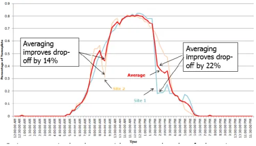
Figure 1: Two separate projects on May 1st shown in blue and yellow and the average of the two shown in red. Time
is on the x-axis and percentage of nameplate production is on the y-axis.
As seen in figure 1, there are two major drops in the day which on their own are very
severe. When averaging the two projects, the effect of the individual drops is much less
pronounced. For a supplier who is interested in providing as close to the potential maximum at
all times without severe drop offs, they may benefit by combining the output of both projects
before dispersing to achieve the smoother average.
Project aggregation is a factor which may help reduce variability in solar output by
employing the Law of Large Numbers, suggesting that as more panels are connected, the average
of the combined output will approach the population mean for all respective time intervals. The
7
one random cloud could not block out all panels if placed farther apart and give a higher average
output than if placed side by side.
Therefore this study seeks to assess the hypothesis that both aggregation and increased
distance between projects are positive factors for the reliability of solar output. The present study
wishes to identify a minimum number of panels for which variability is decrease and production
increase and determine the quantitative effect of distance within those samples.
1.2 Methods
To ease understanding of the project flow and findings the paper has been organized
chronologically. The first section describes the initial data exploration and development of the
basic framework with the use of smaller data sets. The following portion describes the testing
and results on a larger data set which allowed for more conclusive findings. The final section
contains an expansion from the initial model into sub-models in search of a better explanatory
power and understanding of solar output.
2. Data exploration with SPVP & CREST Data Set
The 141 solar projects used in this study contained projects from three different solar
incentive programs. 115 projects came from the California Solar Initiative (CSI) program, a
rebate program based on production levels. Of the remaining 26 projects, 22 come from
California’s Solar Photovoltaic Program (SPVP), a program incentivizing sale of energy
production from midrange solar producers to California utilities (Southern California Edison).
The remaining 4 projects are from the California Renewable Energy Special Tariffs program
(CREST), a feed in tariff program (Southern California Edison). The CSI data set was the
8
were crafted using the SPVP and CREST data. All data sets were provided for the study by
Southern California Edison (SCE), a California based utility.
2.1 Data Cleaning for SPVP & CREST
SCE’s Solar Photovoltaic Program (SPVP) provided data from 22 projects for an interval
of one year. Although data was provided beginning May 21st, 2012, not all projects began on
May 21st. In total 9 of the 21 projects had 15 minute interval production data for all days in the year, while 12 of the remaining projects had data for only a portion of the year. One project did
not return any data in the year interval and was eliminated from the data set. SCE’s CREST
program also provided data for 5 projects for a one year interval. Approximately 5% of the data
set contained errors due to a faulty control box. These portions of data were removed entirely.
The SPVP data were recorded in five minute intervals and in MW. While the CREST data were
recorded in 15 minute intervals and kWh. All data were converted to 15 minute intervals and
MW values as described below.
The data were then normalized by turning each data point into a percentage of their
nameplate, the potential DC production rating, dividing each 15 minute interval by the nameplate
value given by the data providers. The percentage was multiplied by 100 for ease of visual
inspection. As a percentage, each interval becomes a measure of efficiency, which is more
appropriate for the present study than absolute production values.
2.2 Identifying Daily Weather within SPVP & CREST
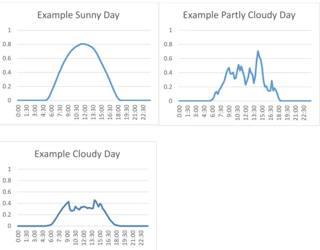
Sunny days are qualitatively described as days with an envelope resembling a normal
diurnal solar radiation pattern based on production levels shown in figure 2a, with a steady rise
9
days. Partly sunny days have distributions which show numerous peaks and troughs, but have
peaks which fall at, slightly below, or above the expected solar production at the time of the
peak. Cloudy days can either be days with little or no production, or days with high volatility and
peaks that fall significantly short of reaching the expected solar production at the time of the
peak.
Figure 2a-c: The daily solar profile of the three different types of days defined in the present study. The x-axis of all graphs shows the time of day while the y-axis shows the percent of nameplate production level.
The three different types of days shown in figure 2a-c were identified by calculating a
daily value which quantifies the variability seen throughout the day. To do this a summation of
the squared differences between consecutive time intervals was calculated, and in order to not
add in a penalty for the natural growth of solar insolation throughout the day, only differences
0 0.2 0.4 0.6 0.8 1
0:00 1:30 3:00 4:30 6:00 7:30 9:00 10:30 12:00 13:30 15:00 16:30 18:00 19:30 21:00 22:30
Example Sunny Day
0 0.2 0.4 0.6 0.8 1
0:00 1:30 3:00 4:30 6:00 7:30 9:00 10:30 12:00 13:30 15:00 16:30 18:00 19:30 21:00 22:30
Example Partly Cloudy Day
0 0.2 0.4 0.6 0.8 1
10
between intervals which oppose the expected direction of growth were included in the
summation. For example, if the data showed a decrease between 10:00 and 10:15, this negative
value was contributed to the sum squared error for the day, as solar production is increasing
during the morning and thus should have been positive in that moment. However, if the data
showed a decrease between 4:00 and 4:15, this would not count towards the sum-squared error
value as the solar production is expected to fall during the afternoon. The average peak time or
solar noon is 12:30, so 12:30 was established as the peak for all days. Differences were expected
to be positive before 12:30 and negative after 12:30. The result of this analysis method is a single
statistic per day which corresponds to the volatility of a solar distribution across all time intervals
within the day. These numbers were used relative to one another to identify if the day was sunny,
partly cloudy or fully cloudy.
This method was developed as part of the present study with the help of Justin Kubassek
and Carl Silsbee, two employees at Southern California Edison. This method is not supported in
other literature, so at every step the data was quantitatively and visually checked to make sure
that the approach was doing what it was intended to do.
2.3 Calculating Weekly Averages
In order to measure variability in solar output, there must be a quantifiable ideal solar
profile to compare with, so the deviation from the ideal, represented in solar variability can be
identified. To do this sunny days were identified using the metric above and averaged together to
make an “ideal” sunny day. With all directional sum-squared differences compiled on one
spreadsheet, a cutoff value for the amount of variability which sunny days must be below were
determined by taking into account the mean and visual tests to see the variability represented by
11
create clean averages at the expense of limiting the sample size. Summing the difference mostly
penalized partly cloudy days which see rapid jumps in production as clouds obstruct the sun, this
metric inappropriately favors cloudy days which have production levels which remain low for
the entire day, and therefore do not have deviations of large magnitudes. Therefore, a maximum
production value was of 60% was added to eliminate days which only had low sum-squared
difference because there were heavy clouds. Using those two criteria a population of just solar
projects which recorded sunny profiles were isolated. Through data exploration it was found that
an “ideal” sunny day for any given month will deviate enough from sunny days at the beginning
or end that those days may not be regarded as sunny. For this reason data from across weeks
were averaged together to create ideal sunny days corresponding to every week.
2.4 Determining Deviation from Sunny Day with SPVP & CREST
With weekly averages established, a quantitative value for deviation from the sunny
weekly average was determined by finding the sum-squared error between each day of collected
data versus the average for the corresponding week. The sum-squared errors for the all projects
over the year of data fell between 1.71 and 54.88 with an average of 11.88 and standard
deviation of 7.58. Each day contains 96 fifteen minute intervals. Average sum-squared error
vales were determined using the assumption that each day produces electricity for sixty
15-minute time intervals, with the remaining 36 intervals recording no value. For example, if an
average deviation of 10% were to be calculated, this would mean that each of the 60 intervals
which recorded a production value would have a difference of 10% and thus show a value of +10
or -10 when subtracting from the mean. Using quantitative cutoffs determined mostly by visual
confirmation, sunny days were selected to contain an average error of no more than 7.5% over 15
12
thus determined to comprise all days with 7.5% average error from average weekly value to 30%
average error, representing 72.5% of all data. Cloudy data represents the final range, all values
with average error above 30%, making up 8.6% of the total days.
The SPVP & CREST data set was not used to make conclusions but merely used as an
exploratory data set, which was necessary due to its smaller size allowing for visual confirmation
at all stages. The framework developed with the SPVP & CREST data sets was used throughout
the study on the more robust CSI data set.
3. Effect of Distance and Aggregation: Testing with CSI Data Set
3.1 Summary of Data Set
The California Solar Initiative (CSI), a program throughout the State of California which
offers production based payments for photovoltaic solar panels, provided a data set consisting of
115 projects from across California (California Public Utilities Commission). The projects are
geographically diverse, stretching from the Sacramento area to the San Diego area, with
13
Figure 3: Map of California’s climate zones with boxes indicating the number of projects in each climate zone found in the CSI data set.
The data set contains 15 minute interval data from May, 2012- April 2013 with
approximate location of the project and DC nameplate rating of each solar project. The
nameplate ratings ranged from residential scale, around 2.1 kW, to industrial size of 1.12 MW.
The California Solar Initiative Organizational team within Southern California Edison supplied
153 projects, out of the 1275 total projects, a random sample representing 12% of the total
population.
3.2 Cleaning and Preparing CSI Data Set
Out of the 153 153 projects were provided, however only 115 were suited for futher use
in the study. Thirty-eight of the projects had no recorded output for the selected year range. This
is due to some of the randomly selected projects have completed the 60-month duration of the
14
data set. An additional seven projects were missing crucial information to the study such as
location or DC nameplate rating. These projects were elminated entirely, as without that data
they could not answer the questions outlined in the goal & scope.
The remaining 115 projects were cleaned. Days with strings of idential numbers repeated
longer than two hours were attributed to meter errors and those project-days were deleted
entirely. Days with a production level of zero for majority of day were deleted. This was decided
as clouds and other weather patterns lead to a decreased solar output but not entire cancelling out
of solar production. Therefore recorded levels of zero were likely due to a obstruction such as a
tree or building, the effect of which is outside the scope of the present study.
The clean project days were then normalized by dividing all production intervals by DC
nameplate rating. This gives a percentage of potential at all intervals during the day, which
allows for largescale anaylsis when grouping projects with production levels differing by almost
1 MW.
3.3 Effect of Aggergation and Distance on Daily Variability
3.3a Creating the Sample
In order to determine the variability of any given day, a benchmark for what to expect
must first be developed. Therefore a “ ideal” sunny day was needed, and was found using the
sunny day metric developed in the early portion of the study using the SPVP & CREST data sets.
As the solar insolation levels change noticably each month, one “typical sunny day” was found
for each week. For a full description on how sunny days were identified refer to section 2.4.
Selection for sunny days was set to only use days with a Sum of Squared error less than
15
value above 75% of nameplate. These cutoffs were strict in order to only isolate days that were
fully sunny, and just 96 days were selected with at least one in each week. A visual inspection
ensured that all of these days had a solar profile extremely close to the ideal.
Using the “ideal” sunny days of each week, deviation from the ideal was measured to
quantify the difference from the sunny day production average of each project experienced each
day. Days were chosen by first dividing the year into four sections by month and selecting 25
random days in each quarter to ensure that 100 days were chosen without a bias for season. Then
for each of the days, a random combination of two samples was chosen. The production value of
both projects were averaged together for every 15-minute interval, to create an entire solar
profile which was an average of the two for the entire day. On each of the 100 days 50 samples
of two random projects were selected and averaged in the same way. This was repeated for
sample sizes 5, 10, 25, and 50. Thus the final data set had 25000 samples.
For each of the samples, the average sunny day was used as a benchmark. The sum of
sqare error of each averaged 15-minute interval of the selected combinations from the “ideal”
sunny day for the corresponding week was computed. Sum of square error, is simply the
summation of the difference between the chosen combination of projects and what the ideal
sunny pattern was for that week, squared. The formula is ∑23:45𝑖=0:00(𝑆𝑎𝑚𝑝𝑙𝑒 𝐷𝑎𝑦𝑖 −
𝐼𝑑𝑒𝑎𝑙 𝑆𝑢𝑛𝑛𝑦 𝐷𝑎𝑦𝑖), where i progresses in 15 minute intervals.
In addition to the sum of square error of the combination from the ideal sunny day, the
sum of square error from the ideal sunny day was computed for each of the individual projects
that comprise the combination. This gave a basis for comparison and allowed improvement to be
quantified by showing the percent improvement from the average of the individual projects to
16
Figure 4: Example of calculation of average distance in a sample of combination size 3.
The average distance between the projects in the combinations was also calculated. All
pair-wise combinations of projects were found and the distance between each is calculated. The
average is then computed by dividing by the total numbers of project pairs.
3.3b Effect of Aggergation on Daily Variability
Aggregation showed a signficant improvement in variability both when grouping by
17
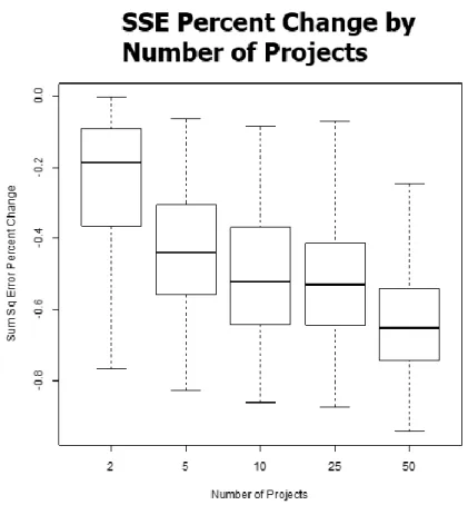
Figure 5: SSE Percent Change by Number of Projects to Show Effect of Aggregation
Figure 5 shows that when combining two projects there is a 19.6% improvement in
deviation from the ideal sunny envelope compared to the average if the two projects were routed
directly to an end use without combining their output. When combining together 5 projects there
is 46% improvement over the individual projects in deviation from the ideal sunny day for the
corresponding week compared to the individual projects without combinations. Beyond
combinations of 5 projects there is increasing improvement, however that improvement per
18
Figure 6: SSE Percent Change Controlling for the Effect of Seasons
Controling for season, to make sure this trend is not dependent on the changes in weather
that occur naturally, there still appears to be a large increase when combining five projects
together compared to the five projects without a combination. From there the improvements of
adding more projects appears to decline athough it is always benefitial to decreasing variability
to add more projects. The winter months appear to have the least improvements from
aggregation across the board, which suggests less variables days involving party cloudy skies. In
spring and summer the improvement is incredibly pronounced. This is likely due to the patchy
cloud cover which is common in the morning and sometimes through the afternoon in Southern
California.
Both the full results, and when controlling for season show that aggregation of projects
19
significant decreases greater than 40% in variability the output from at least five projects must be
combined.
3.3c Effect of Distance on Daily Variability
Next the effect of distance between the projects in the variability of the average sola
profile of the combination was determined. This was found by looking within the samples taken
before and performing an OLD regression using distance to predict SSE change to determine the
significance and explanatory power of distance on variability.
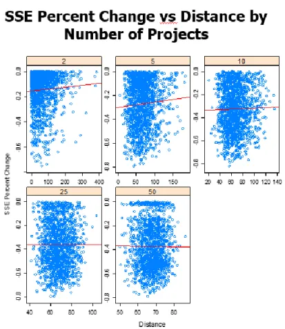
Figure 7: Simple Linear Regression of Distance vs SSE Percent Change by Number of Projects
Figure 7 shows graphically that a linear regression line has no significant explanatory
20
accurate regression as the weather changes daily without regard to distance, and thus two days
cannot be regressed in the sample if the coefficent of determination or coefficent need to be
intrepreted. To examine the true explanatory power of distance, Excell’s correlation function was
used to return the Pearson Correlation Coefficent for the correlation between distance and SSE
percent improvement for each day.
Figure 8: Pearson Correlation Coefficent for Distance vs SSE Percent Improvement by Number of Projects in the Combination
As Pearson’s Correlation Coefficent is equivilent to the square root of 𝑅2, the coeffient of
determination, it can be seen without closer examination that the effect of distance has no
significant explanatory power on SSE percent improvement. To test the significance analytically,
the t-statistic corresponding to the significance of the regressor is run with the following
specifications: 𝐻𝑜: 𝑏1 = 0, and alternative hypothesis, 𝐻𝑎: 𝑏1 ≠ 0, where 𝑏1 is the coefficent
21
𝑏0 is the intercept. The results show that the coefficent value, 𝑏1, is significant for only 9 of the
regressions. And of those significant regressions, the coefficent is almost equally likely to be
positive as negative. This shows that even when distance does have an effect on SSE percent
improvement, the effect is not always a positive one as first hypothesized. For the vast majority
of days and combinations distance appears to be irrelevant.
3.4 Effect of Aggregation on Weekly Minimum
3.4a Creating the Sample
In order to test the effect of aggregation and geographic diversity on weekly minimum,
sub samples of the total data was collected. The samples groups were chosen by taking random
drawings of 2, 5,10, 25 and 50 projects. This sampling was repeated 100 times for each sample
size, for every week in the year, resulting in 26,500 total samples. From those samples, statistics
were calculated based on the projects’ location and efficiency of output.
To test weekly minimum, an on-peak time was chosen, as this is the time when a utility
company most relies on the solar output, it is most interested in improving. 3:00-3:15 was chosen
as the on-peak interval although any 15 minute interval from 2-4 could have been selected. A
breif analysis of toher intervals confirmed 3:00-3:15 to be a fiar representaiton for on-peak
production. The average output of all the panels in each a combination were calculated for
3:00-3:15 for one day. That process was then repeated for every day in the week, and the lowest value
for the week was selected. This was done to determine the most extreme dips in production,
which are the times that a utility company required to supply constant power are most interested
22
time. Averge distance between projects in the combinations was calculated again as it was in
section 3.3a.
3.4b Effect of Aggregation on Weekly Minimum
The effect of aggregation was tested by controlling for seasons and number or projects,
and examining the sum of square error from the typical sunny day for the corresponding week.
For comparison, a random sample of 100 projects was selected for every week and the weekly
minimum was found among that sample.
Figure 9: Improvements in Weekly Minimum due to Aggregation
The results show a modest benefit from aggregation, rasing the extremely weekly
minimum values from 28.49% of nameplate for individual projects to 30.32% for combinations
of two, and to 32.11% for combinations of five projects. After combination size of five projects
23
benefits of aggregation and increase weekly minimums by just under 4% on average a utility
should combine five projects together.
3.4c Effect of Distance on Weekly Minimum for Full Data Set
The results show a negligible correlation between distance and average weekly minimum
production for almost all of the weeks and combination sizes analyzed. Below is a random
selection of weeks to give a visual example to the regressions.
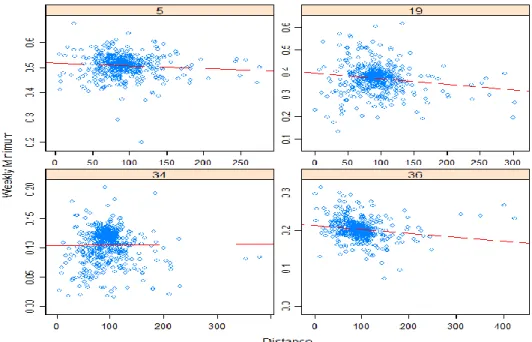
Figure 10: Distance vs Weekly Minimum for Four Random Weeks. None of the correlations are significant.
The line though the clustered data is the line of best fit, and shows that there is a
negligible slope as well as a poor fit for the trend line in all four days. The correlation between
the weekly minimum production values and average distance is calculated based on the data
returned from the 100 combinations of each sample size per week. The data is thus separated by
week and number of projects in combination, and a regression is run independently for each of
24
weeks shown above, creating a necessity for averages to summarize the overall results. The
average correlation by number of projects combined shows very low negative correlation results.
Figure 11: Summary of the Pearson Correlation Coefficient for Distance vs Weekly Minimum
The person correlation coefficient for is 0.076 for two projects, 0.090 for 5 projects,
-0.059 for 10 projects, -0.064 for 25 projects and -0.070 for 50 projects. This shows that over the
entire sample increases in distance do not have a statically relevant impact on weekly minimum.
This is valid within the distance range tested in the present study, from 10- 150 miles.
3. 5 Effect of Distance on Daily Solar Production Values
While distance did not have a significant effect on the weekly minimums, an low-end
extreme, the effect of distance on an average day is potentially significant. To examine the effect
of distance and average daily production, only a comparison between two and five projects was
25
distance between projects begin to show significantly less diversity beyond combinations of five
projects in the previous samples. This due to the properties of averaging outlined in the Law of
Large Numbers, which states that as the number of observations being averaged increases, the
resulting average trends towards the population mean. Beyond five projects the effect of distance
was becoming harder to discern due to the Law of Large Numbers. Additionally, aggregation
results have shown that combinations of five projects are ideal to reduce variability in increase
weekly extremes, so larger combination sizes are not necessary to test. For the reminder of the
study only project combinations of two and five are considered.
3.5a Creating the Sample
Average distance between projects and the average production was calculated for 60
samples of size 2 and 5 for every day of the year. The two statistics were regressed vs one
another to determine the explanatory power of distance on average daily production. In total, 722
total regression were run with the summary results shown below.
26
Figure 12: Pearson Correlation Coefficient of Average Distance vs Average Daily Solar Output
This box-whisker plot above shows the correlation between distance and solar production
is largely negligible. The correlation is slightly negative throughout, and the majority of
correlation values which fall close to zero are statistically insignificant when examining their
t-statistic at the 95% significance level. There are 12 days with significant regressions
combinations of two projects and 7 days with significant regressions for combinations of 5
projects as shown in the 1st and 4th quartile. These significant regressions however balance
themselves out, with an average Pearson correlation coefficient of 0.004462 and 0.003755
respectively of just the significant coefficient values. This shows that even when there is a
statistically significant effect of distance, the effect is just as likely to be negative as it is to be
positive. However roughly 98% of the days tested did not show any statistically significant effect
of distance. These conclusions are only valid where there is appropriate data per day, and while
some days do possess distance above 150 mile and below 10, most days do not. Therefore the
conclusions found above can only be assumed true within an average distance of 10-150 miles.
This expands on the earlier intuition that in addition to not impacting the weekly
minimum, an extreme production value, the average distance between panels in a combination
does not impact the daily production output from solar panels in combinations, a less extreme
consideration.
3.6 Effect of Distance within Climate Zones
3.6a Rationale and Sample Used
As mentioned in the description of the CSI data set, the selection of data sampled
27
can be very severe, switching from cooler and cloudier coastal climates to fully hot and sunny
desert climates within a distance as small as 10 miles, split by geographic boundaries such as
mountains. This creates a potential unexplained variable in the regression, where, for example,
two projects 3 miles apart from each other in the desert would have a better average return than if
one of those projects was connected to another project 10 miles away, in a cloudy climate zone.
To account for this the population was segmented, looking at combinations of 2 and 5 projects in
the three climate zones which contain more than 30 projects.
3.6b Results
Figure 13: Pearson Correlation Coefficient for Figure 14: Pearson Correlation Coefficient for Distance vs Average Daily Output for Climate Distance vs Average Daily Output for Climate
Zones 8, 9 and 10 for 2 projects Zones 8, 9 and 10 for 5 projects.
The data shows that even when examining within a climate zone, there appears to be an
insignificant effect on production output for an increased distance. Again the majority of the
28
722 regressions run for each of the three climate zones, 51 days in climate zone 8, 52 days in
climate zone 9, and 47 days in Climate zone 10 have regression of distance vs average
production which are statistically significant at the 95% level. The average of the person
correlation coefficient however is -0.02384, -0.03616, and 0.02562 respectively. This shows that
when looking at the entire year, there are days when distance does have statistically significant
effect. However, the result of this effect is as likely to be a positive effect as it is to be a negative
effect. The acceptable distance range here falls within 10-85 miles, representing a smaller area
than before due to the upper bound on project pairs now.
In comparison to the full model, which allowed for combinations between projects in
multiple climate zones, the main difference is that there are more days in which distance has a
statistically significant effect for the regressions run in any one of the three climate zones. This
suggests that distance is more likely to have an effect when expanding within a similar climate.
However, like before this effect is just as likely to be positive as to be negative.
3.7 Effect of Distance on Partly Cloudy Days
As the qualitative motivation for examining distance was to determine if a larger distance
between projects could help escape from local cloud cover in partly cloudy days, such that all the
panels in a combination would not be covered by a cloud at the same time. To more directly test
this idea, partly cloudy days were isolated and the effect of distance was determined in only days
that are considered party cloudy.
3.7a Creating the Sample
The method for identifying days was developed with the test SPVP & CREST data set.
29
except lower cutoffs were used to isolate the imperfect partly sunny days. A high daily max was
required of all projects isolated to ensure that projects were not fully or almost fully cloudy.
Once projects days which were partly cloudy were isolated and a visual inspection confirmed
that appropriate days had been selected, the days which contained more than 50 projects with
partly cloudy solar profiles were used to regress average distance vs average production. There
were 42 days with a large enough project population to justify a regression model.
3.7b Results
On the full model there did not appear to be any significant correlation, however a visual
inspection showed that there was an effect of distance outliers which skewed the model. Therefor
the model was again separated into climate zones. Out of the three main climate zones, only two
had populations of partly cloudy days high enough to run regression models. The summary
statistics for the 42 regressions run for each size in both climate zones.
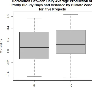
Figure 15: Pearson Correlation Coefficient for Figure 16: Pearson Correlation Coefficient for
30
Days for Climate Zones 9 and 10 for 2 projects Days for Climate Zones 8, 9 and 10 for 5 projects.
The results once again appear to be insignificant, with a very low median Pearson
correlation coefficient. Again the correlation coefficients were screened for significance and for
combination size two, nine days contained significant correlation coefficients in climate zone 9
and four days in climate zone 10. For combination size five, seven days contained significant
correlation coefficients in climate zone 9 and seven days also contained significant correlation
coefficients in climate zone 10. In this model the significant regression have a far higher
coefficient value and 𝑅2. For two projects in climate zone 10, the 𝑅2 on partly cloudy
statistically significant days was 0.287 on average. For five projects in climate zone 9 it was
0.2602 and for five projects in climate zone 10 it was 0.1748 on average. For two projects in
climate zone 9 it was too small to be significant. These coefficients of determination are far from
conclusive in regard to the link between distance and solar output, however is does suggest that
there are a few select days, likely in the range of 1 dozen per year, in which weather conditions
are right such that a greater distance between projects will lead to a higher solar output. The
average coefficient values associated with the statistically significant partly cloudy days were
0.002919 for five projects in climate zone 9, 0.001664 for two projects in climate zone 10 and
0.003716 for five projects in climate zone 10. These coefficients can be interpreted as a one mile
increase between the averages of the five panels in climate zone 9 leads to a 0.002919% increase
in the combined average solar output, and similarly for the other coefficient values.
It should be noted however, that roughly 90% of partly cloudy days tested did not have
significant effect of distance. These results simply say that despite being anomalous to the norm,
31
between projects within one climate zone are within 10- 85 miles. Therefore these coefficient
values are only valid within that range.
3.8 Effect of Distance among Adjacent Projects
The present study has shown through regressions on various subsamples that an average
distance between projects of 10- 150 miles for the full samples, and 10- 85 miles within one
climate zone, distance is largely insignificant. However, the effect of distance among solar sites
placed less than 10 miles from one another has not been sufficiently explored.
Finding the effect of these small distances is difficult in the present data set, as taking a
subsample of distance under 10 miles leads to a sample size under 10 observations, which too
small to draw conclusions based off of. However since it has been shown that within the distance
range of the project, spacing is insignificant the data does allow us to examine the effect of
moving from adjacent projects to a combination of the same size at an arbitrary distance, at least
10 miles apart.
Figure 17: Average Daily Solar Production By Number of Figure 18: Weekly Minimum Solar Production by Number
Projects where distance is arbitrary between of projects where distance is arbitrary between
32
The plot showing average daily solar production shows that on average adjacent projects
will return the same value as projects in combinations with an average distance between 10-150
miles. The 1st and 3rd quartile lines show that the combinations with distance between them give are more consistent output, as was shown in the aggregation sections. The primary benefit of
placing space between adjacent projects is the increase in the average weekly minimum value,
which can be increased roughly 4% by making the average space between the projects in the
combination at least five miles. This shows that although there has been no significant impact of
distance within the sample tested, there is a benefit of distance when expanding from adjacent
projects.
Looking at the regressions for combinations of 5 projects, the results appear conclusive
that within a distance range of 10- 150 miles, distance is insignificant. However the results
discussed above prove that there is a negative effect of placing projects side by side. The present
data set however does not have sample sizes lager than 10 for combinations of projects at
distances under 10 miles, which is not a large enough sample to make conclusions based upon.
Therefore results for this crucial range, to determine at what point average distance further
increases become insignificant, are inconclusive. Therefore the present study is forced to
recommend that projects are formed with an average distance of at least 10 miles between
projects.
4. Summary of Results
The present study sets out to answer two questions: is combining the output of projects
33
return? And what quantifiable effect does the distance between projects in those combinations
have on solar output? The main metrics to assess the improvement were overall daily variability
and solar output at peak. It was found through both metrics that aggregation was incredibly
effective at ensuring a higher and more reliable solar output. It was found that to decrease
extreme weekly minimum at peak demand, a combination of five panels I also necessary. It is
assume that these projects would be “combined” by simply grouping their output at some staging
station such as a local power station before sending it to the end use. Therefore the present study
suggest that at least five projects are aggregated to ensure a steady and reliable output.
The present study proved that distance does not have a significant effect on reliability and
output of solar panels between 10 and 150 miles. Looking at the entire data set, days when there
is a significant impact of average distance in a combination are rare. When examining the
segmented sample within one climate zone, the effect of distance was insignificant. For this
model, roughly 10 out of 365 days contained correlation coefficients for distance which were
significant, and there was no trend towards positive or negative coefficient values. The study
found that on partly cloudy days, within days where the coefficient value on distance is
significant, distance is more likely to have a positive effect on production at peak. This is the
only instance where distance is found to have any significant effect in one direction, and even in
this instance the coefficient of determination is within the range of 0.30-0.25 for the differing
climate zones and combination sizes. Thus, based on the finding of the study it can be concluded
that distance between 10 and 150 miles does not have a substantial effect on solar output. Even
on partly cloudy days when distance may lead to increased output levels, there are other days
during the year when distance between projects leads to a lower output level. Finally, these days
34
data across the entire year. In all samples no more than 10% of the days showed any significant
impact for distance. Qualitatively this can be explained by the fact that clouds are random, and
when combining panels there is no sure method to ensure that the area, when the distance is
above ten miles apart, is not also under cloud cover. The only positive effect from distance
shown is to combine projects which are not adjacent. However, the current data set does not
allow a full assessment of the effect of distances under 10 miles. With the negative effect shown
for projects placed adjacent to one another and the insignificant effects of increased distance
between 10 and 150 miles it can be seen that the improvements caused by distance have ceased
by the point average distance reaches 10 miles. Therefore, although further study to determine
the effect of distance at distances under 10 miles is recommended, the present study recommends
that within the combinations of size 5, an average distance of 10 miles is maintained.
Works Cited
1. California Public Utilities Commission. (March, 2013 26).About the california solar iniative. Retrieved from http://www.cpuc.ca.gov/puc/energy/solar/aboutsolar.htm
2. Southern California Edison. (March, 2013 24). Renewable & alternative power - spvp-ipp. Retrieved from https://www.sce.com/wps/portal/home/procurement/renewable-alternative-power-contract-opportunities/svpvp-ipp/