Safe Probability
Peter Gr¨unwald April 8, 2016
Abstract
We formalize the idea of probability distributions that lead to reliable predictions about some, but not all aspects of a domain. The resulting notion of ‘safety’ provides a fresh perspective on foundational issues in statistics, providing a middle ground between imprecise probability and multiple-prior models on the one hand and strictly Bayesian approaches on the other. It also allows us to formalize fiducial distributions in terms of the set of random variables that they can safely predict, thus taking some of the sting out of the fiducial idea. By restricting probabilistic inference to safe uses, one also automatically avoids paradoxes such as the Monty Hall problem. Safety comes in a variety of degrees, such as ‘validity’ (the strongest notion), ‘calibration’, ‘confidence safety’ and ‘unbiasedness’ (almost the weakest notion).
1
Introduction
We formalize the idea of probability distributions that lead to reliable predictions about some, but not all aspects of a domain. Very broadly speaking, we call a distribution ˜P safe for predicting random variableU given random variable V if predictions concerningU based on
˜
P(U|V) tend to be as good as one would expect them to be if ˜P were an accurate description of one’s uncertainty, even if ˜P may not represent one’s actual beliefs, let alone the truth. Our formalization of this notion of ‘safety’ has repercussions for the foundations of statistics, providing a joint perspective on issues hitherto viewed as distinct:
1. All models are wrong...1 Some statistical models are evidently both entirely wrong yet very useful. For example, in some highly successful applications of Bayesian statistics, such as latent Dirichlet allocation for topic modeling (Blei et al., 2003), one assumes that natural language text is i.i.d., which is fine for the task at hand (topic modeling) — yet no-one would want to use these models for predicting the next word of a text given the past. Yet, one can use a Bayesian posterior to make such predictions any way — Bayesian inference has no mechanism to distinguish between ‘safe’ and ‘unsafe’ inferences. Safe probability allows us to impose such a distinction.
2. The Eternal Discussion2 More generally, representing uncertainty by a single distri-bution, as is standard in Bayesian inference, implies a willingness to make definite predictions about random variables that, some claim, one really knows nothing about. Disagreement on
1...yet some are useful, as famously remarked by Box (1979). 2
When the single-vs. multiple-prior issue came up in a discussion on thedecision-theory forum mailing list, the well-known economist I. Gilboa referred to it as ‘the eternal discussion’.
this issue goes back at least to Keynes (1921) and Ramsey (1931), has led many economists to sympathize withmultiple-prior models (Gilboa and Schmeidler, 1989) and some statisticians to embrace the related imprecise probability (Walley, 1991, Augustin et al., 2014) in which so-called ‘Knightian’ uncertainty is modeled by a set P∗ of distributions. But imprecise
probability is not without problems of its own, an important one being dilation (Example 1 below). Safe probability can be understood as starting from a setP∗, but thenmapping the set of distributions to a single distribution, where the mapping invoked may depend on the prediction task at hand — thus avoiding both dilation and overly precise predictions. The use of such mappings has been advocated before, under the name pignistic transformation
(Smets, 1989, Hampel, 2001), but a general theory for constructing and evaluating them has been lacking (see also Section 5).
3. Fisher’s Biggest Blunder3 Fisher (1930) introduced fiducial inference, a method to
come up with a ‘posterior’ ˜P(θ |Xn) on a model’s parameter space based on data Xn, but without anything like a ‘prior’, in an approach to statistics that was neither Bayesian nor frequentist. The approach turned out problematic however, and, despite progress on related
structural inference (Fraser, 1968, 1979) was largely abandoned. Recently, however, fiducial
distributions have made a comeback (Hannig, 2009, Taraldsen and Lindqvist, 2013, Martin and Liu, 2013, Veronese and Melilli, 2015), in some instances with a more modest, frequentist interpretation asconfidence distributions (Schweder and Hjort, 2002, 2016). As noted by Xie and Singh (2013), these ‘contain a wealth of information for inference’, e.g. to determine valid confidence intervals and unbiased estimation of the median, but their interpretation remains difficult, viz. the insistence by Hampel (2006), Xie and Singh (2013) and many others that, although ˜P(· |Xn) is defined as a distribution on the parameter space, the parameter itself is not random. Safe probability offers an alternative perspective, where the insistence that ‘θis not random’ is replaced by the weaker (and perhaps liberating) statement that ‘we can treat θas random’ as long as we restrict ourselves to safe inferences about it’ — in Section 3.1 we determine precisely what these safe inferences are and how they fit into a general hierarchy:
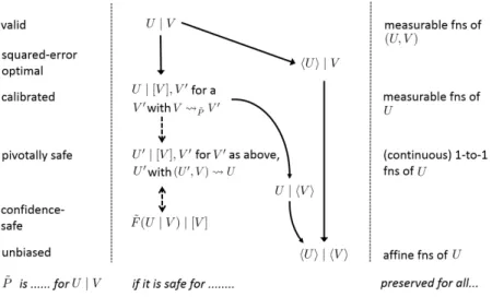
4. The Hierarchy Pursuing the idea that some distributions are reliable for a smaller subset of random variables/prediction tasks than others, leads to a natural hierarchy of safeties — a first taste of which is in Figure 1 on page 5, with notations explained later. At the top are distributions that are fully reliable for whatever task one has in mind; at the bottom those that are reliable only for a single task in a weak, average sense. In between there is a natural place for distributions that are calibrated (Example 2 below), that are
confidence–safe (i.e. valid confidence distributions) and that are optimal for squared-error
prediction.
5. “The concept of a conditional probability with regard to an isolated hypoth-esis...4 Upon first hearing of the Monty Hall (quiz master, three doors) problem (vos Savant, 1990, Gill, 2011), most people naively think that the probability of winning the car is the same whether one switches doors or not. Most can eventually, after much arguing, be
3While Fisher is generally regarded as (one of) the greatest statisticians of all time, fiducial inference is
often considered to be his ‘big blunder’ — see Hampel (2006) and Efron (1996), who writesMaybe Fisher’s biggest blunder will become a big hit in the 21st century!
4
convinced that this is wrong, but wouldn’t it be nice to have a simple sanity check that
im-mediately tells you that the naive answer must be wrong, without even pondering the ‘right’
way to approach the problem? Safe probability provides such a check: one can immediately tell that the naive answer is not safe, and thus cannot be right. Such a check is applicable more generally, whenever conditioning on events rather than on random variables (Example 4 and Section 4).
6. “Could Neyman, Jeffreys and Fisher have agreed on testing?5 Ryabko and Monarev (2003) shows that sequences of 0s and 1s produced by standard random number generators can be substantially compressed by standard data compression algorithms such asrarorzip. While this is clear evidence that such sequences are not random, this method is neither a valid Neyman-Pearson hypothesis test nor a valid Bayesian test (in the tradition of Jeffreys). The reason is that both these standard paradigms require the existence of an
alternative statistical model, and start out by the assumption that, if the null model (i.i.d. Bernoulli (1/2)) is incorrect, then the alternative must be correct. However, there is no clear sense in whichzipcould be ‘correct’ — see Section 5. There is a third testing paradigm, due to Fisher, which does view testing as accumulating evidence againsth0, and not necessarily as
confirming some precisely specifiedh1. Yet Fisher’s paradigm is not without serious problems
either — see Section 5.
Berger et al. (1994) started a line of work culminating in Berger (2003), who presents tests that have interpretations in all three paradigms and that avoid some of the problems of their original implementations. However, it is essentially an objective Bayes approach and thus inevitably, strong evidence againsth0implies a high posterior probability thath1is true.
If one is really doing Fisherian testing, this is unwanted. Using the idea of safety, we can extend Berger’s paradigm by stipulating the inferences for which we think it is safe: roughly speaking, if we are in a Fisherian set-up, then we declare all inferences conditional onh1to be
unsafe, and inferences conditional onh0 to be safe; if we really believe thath1 may represent
the state of the world, we can declare inferences conditional onh1 to be safe. But much more
is possible using safe probability — a DM can decide, on a case by case basis, what inferences based on her tests would be safe, and under what situations the test results itself are safe — for example, some tests remain safe under optional stopping, whereas others (even Bayesian ones!) do not. While we will report on this application of safety (which comprises a long paper in itself) elsewhere, we will briefly return to it in the conclusion.
7. Further Applications: Objective Bayes, Epistemic Probability Apart from the applications above, the results in this paper suggest that safe probability be used to formalize the status of default priors inobjective Bayesian inferences, and to enable an alternative look atepistemic probability. But this remains a topic for future work, to which we briefly return at the end of the paper.
The Dream Imagine a world in which one would require any statistical analysis — whether it be testing, prediction, regression, density estimation or anything else — to be accompanied by asafety statement. Such a statement should list what inferences, the analysists think, can be safely made based on the conclusion of the analysis, and in what formal ‘safety’ sense. Is the alternativeh1 really true even though h0 is found to be false? Is the suggested predictive
5
distribution valid or merely calibrated? Is the posterior really just good for making predictions via the predictive distribution, or is it confidence-safe, or is it generally safe? Does the inferred regression function only work well on covariates drawn randomly from the same distribution, or also under covariate shift? (an application of safety we did not address here but which we can easily incorporate). The present, initial formulation of safe probability is too complicated to have any realistic hopes for a practice like this to emerge, but I can’t help hoping that the ideas can be simplified substantially, and a safer practice of statistics might emerge.
Starting with Gr¨unwald (1999), my own work — often in collaboration with J. Halpern — has regularly used the idea of ‘safety’, for example in the context of Maximum Entropy inference (Gr¨unwald, 2000), and also dilation (Gr¨unwald and Halpern, 2004), calibration (Gr¨unwald and Halpern, 2011), and probability puzzles like Monty Hall (Gr¨unwald and Halpern, 2003, Gr¨unwald, 2013). However, the insights of earlier papers were very partial and scattered, and the present paper presents for the first time a general formalism, definitions and a hierarchy. It is also the first one to make a connection to confidence distributions and pivots.
1.1 Informal Overview
Below we explain the basic ideas using three recurring examples. We assume that we are given a set of distributionsP∗ on some space of outcomesZ. Under a frequentist interpreta-tion, P∗ is the set of distributions that we regard as ‘potentially true’; under a subjectivist interpretation, it is thecredal set that describes our uncertainty or ‘beliefs’; all developments below work under both interpretations.
All probability distributions mentioned below are either an element of P∗, or they are a
pragmatic distribution P˜, which some decision-maker (DM) uses to predict the outcomes of
some variable U given the value of some other variable V,where both U and V are random quantities defined onZ. ˜P is also used to estimate the quality of such predictions. ˜P (which may be, but is not always inP∗) is ‘pragmatic’ because we assume from the outset that some
element of P∗ might actually lead to better predictions — we just do not know which one.
Example 1 [Dilation]A DM has to make a prediction or decision about random variable U ∈ U ={0,1} given the value of V ∈ V ={0,1}. She knows that the marginal probability P(U = 1) = 0.9; she suspects that U may depend on V, but has no idea whether U and V are positively or negatively correlated or how strong the correlation is. She may thus model her uncertainty as the set P∗ of all distributionsP on Z =U × V that satisfy
P(U = 1) =X v∈V
P(U = 1, V =v) = 0.9. (1)
Given thatV = 1, what should she predict forU? A standard answer in imprecise probability (Walley, 1991) is to pointwise condition the set P∗, leading one to adopt the probabilities
P∗(U = 1|V = 1) :={P(U = 1|V = 1) :P ∈ P∗}. But this set containsevery distribution on U, including P(U = 1 | V = 1) = 0 (the latter would obtain for the P ∈ P∗ with P(U = |1−V|) = 1). It therefore seems that, after observing V = 1, the DM has lost rather than gained information. By symmetry, the same happens after observing V = 0, so
whatever DM observes, she loses information— a phenomenon known asdilation(Seidenfeld
Figure 1: A Hierarchy of Relations for ˜P. The concepts on the right correspond (broadly) to existing notions, whose name is given on the left (with the exception ofU | hVi, for which no regular name seems to exist). A →B means that safety of ˜P for A implies safety forB — at least, under some conditions: for all solid arrows, this is proven under the assumption ofV with countable range (see underneath Proposition 1). For the dashed arrows, this is proven under additional conditions (see Theorem 2 and subsequent remark). On the right are shown transformations onU under which safety is preserved, e.g. if ˜P is calibrated for U|V then it is also calibrated for U0 | V for every U0 with
U U0 (see remark underneath Theorem 2). Weakening the conditions for the proofs and providing more detailed interrelations is a major goal for future work, as well as investigating whether the hierarchy has a natural place forcausal notions, such as ˜P(U |do(v)) as in Pearl’s (2009) do-calculus.
ignore V and predict using the distribution that acts as if U ⊥V and has
˜
P(U = 1|V =v) =P(U = 1) for allv∈ V, (2)
i.e. ˜P(U = 1|V =v) = 0.9. While from a purely subjective Bayesian standpoint information is never useless and this seems silly, it is certainly what humans often do in practice, and usually, they get away with it (Dempster, 1968) — for concrete examples see Gr¨unwald and Halpern (2004). Here is where Safe Probability comes in — it tells us that ˜P issafe to use, in the following simple sense: for any function g:U →R, we have:
for all P ∈ P∗, allv∈ V: EU∼P[g(U)] = EU∼P˜[g(U)|V =v]. (3)
In particular, if we have a loss function L : U × A →R mapping outcomes and actions to associated losses, then, for any actiona∈ A, we can plug ing(U) :=L(U, a) above and then we find that (assuming P∗ contains the truth):
DM’s predictions are guaranteed to be exactly as good, in expectation, as she would expect them to be if P˜ were actually ‘true’ — even if ˜P is not true at all.
We immediately add though that if we had a loss function L0 :U × V × A →Rwhich would
itself depend on V (e.g. if V = 1 DM is offered a different bet on U than if V = 0) then
(Definition 1, 2 and 3), this will be expressed as ‘ ˜P is safe for predicting with loss function L but not loss function L0’, or, in formal notation, ˜P is safe for L(·, a) | [V] but not for L0(·, a)|[V]. The intuitive meaning is that DM can safely use ˜P to make predictions against L (her predictions will be as good as she expects) but not againstL0. These statements will be immediate consequences of the more general statements ‘ ˜P is safe forU |[V] but not safe forU |V’.
In some cases, we will not be able to come up with a ˜P satisfying (3), and we have to settle for a ˜P that satisfies a weaker notion of safety, such as, for all P ∈ P∗, all functionsg,
EV∼P
EU∼P˜[g(U)|V]
=EU∼P[g(U)], (4)
which says that DM predicts as well on average as DM would expect to predict on average if ˜
P were true, even though ˜P may not be true. This will be denoted as ‘ ˜P is safe forU | hVi’; and if (4) only holds forg the identity (which makes no difference if|U |= 2, but in general it does) we have the even weaker safety for hUi | hVi (Figure 1). In Section 2.2 we thus obtain five basic notions of safety, varying from weak safety, in an average sense, to very strong safety, safety for U | V, which essentially means that ˜P(U | V) must be the correct conditional distribution.
In this example we used frequentist terminology, such as ‘correct’ and ‘true’, and we continue to do so in this paper. Still, a subjective interpretation remains valid in this and future examples as well: if the DM’s real beliefs are given by the full set P∗, she can safely act as if her belief is represented by the singleton ˜P as long as she also believes that her loss does not depend on V.
Example 3 [Bayesian, Fiducial and Confidence Distributions]We are given a para-metric probability model M= {qθ |θ∈ Θ} where Θ⊆Rk for some k ≥1, each qθ defines a probability density or mass function on data (X1, . . . , XN) = XN of sample size N, each
outcome Xi taking a value in some space X. The goal is to make inferences about θ, based on the data XN or some statistic S(XN, N) thereof. In the common case with fixed N =n and inference based on the full data, S(XN, N) := Xn, we can transfer this statistical sce-nario to our setup by defining P∗ as a set of distributions on Z = Θ× Xn. RVs U and V =S(Xn, n) =Xnare then defined as, for eachz= (θ, xn),U(z) :=θandV(z) :=xn. DM employs a set Π of prior distributions on Θ, where each π ∈Π induces a joint distribution Pπ on Θ× Xn with marginal on Θ determined by π and, given θ, density of xn given by qθ, so that if π has density pπ, we get the joint density pπ(θ, xn) = pπ(θ)·qθ(xn). We set
P∗ :={Pπ :π ∈Π} to be the set of all such joint distributions. In the special case in which DM really is a 100% subjective Bayesian who believes that a single prior π captures all un-certainty, we have that P∗ = {P
π} contains just a single joint parameter-data distribution, and we are in the standard Bayesian scenario. Then DM can set ˜P(θ|Xn) := Pπ(θ |Xn), the standard posterior, and any type of inference about θ is safe relative to P∗. Here we focus on another special case, in which Π contains exactly one density for eachθ∈Θ, namely the degenerate distribution putting all its mass onθ. We denote this distribution byPθ and notice that then P∗ = {Pθ : θ ∈ Θ}, with Pθ(Θ = θ) = 1, and for any measurable set A, Pθ(Xn∈ A) determined by density pθ, satisfying
pθ(xn) =pθ(xn|Θ =θ) =qθ(xn).
Still, any choice of pragmatic distribution ˜P(U | V) = ˜P(θ | Xn) can be interpreted as a distribution on U ≡ Θ given the data Xn, analogous to a Bayesian posterior. In Section 3 we investigate how one can construct distributions ˜P of this kind that are safe for inference about confidence intervals. for simplicity we restrict ourselves to the 1-dimensional case, for which we find that the construction we provide leads to ˜P that are confidence-safe, written in our notation as ‘safe for ˜F(U|V) | [V]’, with ˜F being the CDF (cumulative distribution function) of ˜P(U|V). Confidence safety is roughly the same as coverage Sweeting (2001): it means that the ‘true’ probability that θ is contained in a particular type of α-credible sets (sets with ‘posterior’ probabilityα given the dataV), is equal toα.
The ˜P we construct are essentially equivalent to theconfidence distributions of (Schweder and Hjort, 2002), that were designed with the explicit goal of having good confidence prop-erties; they also often coincide with Fisher’s 1930 fiducial distributions, which in later work (Fisher, 1935) he started treating as ordinary probability distributions that could be used without any restrictions. This cannot be right (see e.g. (Hampel, 2006, page 514)), but the question has always remained how a probability calculus for fiducial distributions could be derived that incorporates the right restrictions. Our work provides a step in this direction, in that we show how such ˜P snugly fit into our general framework: confidence safety is a strictly weaker property than calibration, and has again a natural representation in terms of thehUi | hVinotation mentioned above. Moreover, it is a special case ofpivotal safety which also has repercussions in quite different contexts — see Example 4.
The example illustrates two important points:
which dataV are text corpora,P∗, not explicitly given, is a complicated set of realistic
distributions overV under which data are non-i.i.d., and the literature suggests to take ˜
P(U |V) as the Bayesian posterior for a cleverly designed i.i.d. model.
2. In other cases, DM may want to construct a ˜P herself. In Example 1, the safe ˜P was obtained by replacing an (unknown) conditional distribution with a (known) marginal — a special case of what was called C-conditioning by Gr¨unwald and Halpern (2011). Marginal distributions and distributions that ignore aspects of V play a more central role in this construction process: they also do in the confidence construction mentioned above, where one sets ˜P(U |V) equal to a distribution such that ˜P(U0 |V), whereU0 is some auxiliary random variable (apivot), becomes independent ofV. For the original RV U though, in the dilation example, DM acts as if U and V are independent even though they may not be; in the confidence distribution example, DM acts in a ‘dual’ manner, namely as if U and V are dependent, even though under P∗ they are not — which is fine, as long as her conclusions aresafe.
Example 4 [Event-Based Conditioning and Pivotal Safety via Monty Hall]More generally, we may look at safety for pragmatic distributions ˜P that condition on events rather than random variables. To illustrate, consider the Monty Hall Problem (vos Savant, 1990, Gill, 2011): suppose that you’re on a game show and given a choice of three doors {1,2,3}
Behind one is a car; behind the others are goats. You pick door 1. Before opening door 1, Monty Hall, the host opens one of the other two doors, say, door 3 which has a goat. He then asks you if you still want to take what’s behind door 1, or to take what’s behind door 2 instead. Should you switch? You may assume that initially, the car was equally likely to be behind each of the doors and that, after you go to door 1, Monty will always open a door with a goat behind. Basically you observe either the event{1,3} (if Monty opens door 2) or {1,2} (if Monty opens 3). You can then calculate your optimal decision according to some distribution ˜P({1} | E), where E ∈ {{1,3},{1,2}} is the event you observed. Naive conditioning suggests to take P({1} | {1,2}) =P({1} | {1,3}) = (1/3)/(2/3) = 1/2, and it takes a long time to convince most people that this is wrong — but, if DM’s would adhere to safe probability, then no convincing and explanation would be needed: translation of the example into our ‘safety’ setting immediately shows, without any further thinking about the problem, that this choice of ˜P isunsafe, under all notions of safety we consider! (Section 4). Another aspect of the Monty Hall problem is that, in most analyses that are usually viewed as ‘correct’, one implicitly assumes that the quiz master flips a fair coin to decide whether to open door 2 or 3 if you choose door 1 so that he has a choice. There have been heated discussions (e.g. on wikipedia talk pages) about whether this assumption is justified. In Example 11 we show that the ˜P which assumes a fair coin flip by Monty is an instance of a
pivotally safe pragmatic distribution. These have the properties that for many loss functions
(including 0/1-loss as in Monty Hall), they lead one to making optimal decisions. Thus, while assuming a fair coin flip may be wrong, it is stillharmless to base one’s decisions upon it.
variables. Section 4 briefly discusses non-numerical observations as well as probability updates that cannot be viewed as conditional distributions. We end with a discussion of further potential applications of safety as well as open problems. Proofs and further technical details are delegated to the appendix.
2
Basic Definitions for Discrete Random Variables
For simplicity, we introduce our basic notions only considering countableZ, which allows us to sidestep measurability issues altogether. Thus below,Z is countable; we treat the general case in Section 3.
2.1 Concepts and notations regarding distributions on Z
We define a random variable (abbreviated to RV) to be any function X :Z →Rk for some k >0. Thus RVs can be multidimensional (i.e. what is usually called ‘random vector’). By an ‘Y-valued RV’ or simply ‘generalized RV’ we mean any function mappingZ to an arbitrary set Y. For two RVs U = (U1, . . . , Uk1), V = (V1, . . . , Vk2) where Uj and Vj are 1-dimensional
random variables, we define (U, V) to be the RV with components (U1, . . . , Uk1, V1, . . . , Vk2).
For any generalized RVs U and V on Z and functionf we writeU f V if for all z∈ Z, V(z) = f(U(z)). We write U V (“U determines V”, or equivalently “U is a coarsening
of V”) if there is a function f such that U f V. We write U ! V if U V and V U. For two GRVs U and V we write U ≡ V if they define the same function on Z,
and for a distribution P ∈ Z we write U=PV if P(U = V) = 1. We write U f
P V if P({z ∈ Z:V(z) =f(U(z))}) = 1, and U P V if there exists some f for which this holds. Clearly U V implies that for all distributions P on Z,U P V, but not vice versa. Let S :Z → S be a function on Z. Therange ofS, denoted range(S), the support ofS under a distribution P, and the range of S given that another function T on Z takes value t, are denoted as
range(S) :={s∈ S :s=S(z) for some z∈ Z} ; suppP(S) :={s∈ S :P(S=s)>0}, range(S|T =t) ={s∈ S :s=S(z) for some z∈ Z witht=T(z)} (5)
where we note thatsuppP(S)⊆range(S), with equality if S has full support.
For a distribution P on Z, andU-valued RVU, we write P(U) as short-hand to denote the distribution ofU under P (i.e. P(U) is a probability measure).
We generally omit double brackets, i.e. if we writeP(U, W) for RVsU and W, we really mean P(R) whereR is the RV (U, W),
Any generalized RV that maps allz∈ Z to the same constant is calledtrivial, in particular the RV 0 which maps all z ∈ Z to 0. For an eventE ⊂ Z, we define the indicator random variable 1E to be 1 if E holds and 0 otherwise.
Conditional Distributions as Generalized RVs For given distribution onZ and gen-eralized RVs V and W, we denote, for all v ∈ suppP(V), P | V = v as the conditional distribution onZ givenV =v, in the standard manner. We further define (P∗ |W =w) :=
We further denote, for all v ∈ suppP(V), P(U |V = v) as the conditional distribution of U given V =v, defined as the distribution on U given by P(U = u |V = v) := P(U = u, V =v)/P(V =v) (whereasP |V =v is defined as a distribution onZ,P(U |V =v) is a distribution on the more restricted space range(U)).
Suppose DM is interested in predicting RV U given RV V and does this using some conditional distribution P(U | V = v) (usually this P will be the ‘pragmatic’ ˜P, but the definition that follows holds generally). Adopting the standard convention for conditional expectation, we call any function from range(V) to the set of distributions on U that coincides withP(U |V =v) for all v ∈ suppP(V) a version of the conditional distribution P(U |V). If we make a statement of the form ‘P(U |V) satisfies ...’, we really mean ‘every version of P(U | V) satisfies...’. We thus treat P(U | V) as a E-valued random variable where E = {P(U |V = v) : v ∈ range(V)}, where, for all z ∈ Z with P(V =V(z)) >0, P(U |V)(z) :=P(U |V =V(z)), and P(U |V)(z) set to an arbitrary value otherwise.
Unique and Well-Definedness Recall that DM starts with a set P∗ of distributions on
Z that she considers the right description of her uncertainty. She will predict sume RV U given some generalized RVV using apragmatic distribution ˜P.
For RV U : Z → Rk and generalized RV V, we say that, for given distribution P0 on
Z, P0(U |V) is essentially uniquely defined (relative to P∗) if for all P ∈ P∗,
suppP(V) ⊆ suppP0(V) (so that P-almost surely V takes value v with P0(V = v) > 0). We use this definition both for P0 ∈ P∗ and for P0 = ˜P; note that we always evaluate whether P0 is uniquely defined under distributions in the ‘true’ P∗ though.
We say that EP0[U |V] is well-defined if, writingU = (U1, . . . , Uk), and,U+
j = max{Uj,0}, Uj− = max{−Uj,0}, we have, for j = 1..k, either EP0[U+
j | V] < ∞ with P-probability 1, or EP0[U−
j | V] < ∞ with P-probability 1. This is a very weak requirement that ensures that calculating expectations never involves the operation ∞ − ∞, making all expectations well-defined.
The Pragmatic Distribution P˜ We assume that DM makes her predictions based on a probability distribution ˜P on Z which we generally refer to as thepragmatic distribution. In practice, DM will usually be presented with a decision problem in which she has to predict some fixed RVU based on some fixed RVV, and then she is only interested in the conditional distribution ˜P(U |V), and for some other RVs U0 and V0, ˜P(U0 |V0) may be left undefined. In other cases she only may want to predict the expectation ofU givenV — in that case she only needs to specify EP˜[U | V] as a function of V, and all other details of ˜P may be left
unspecified. In Appendix A.1 we explain how to deal with suchpartially specified P˜. In the main text though, for simplicity we assume that ˜P is a fully-specified distribution on Z; DM can fill up irrelevant details any way she likes. The very goal of our paper being to restrict
˜
P to making ‘safe’ predictions however, DM may come up with ˜P to predictU given V and there may be many RVs U0 and V0 definable on the domain such that ˜P(U0 | V0) has no bearing to P∗ and would lead to terrible predictions; as long as we make sure that ˜P is not
used for suchU0 and V0 — which we will — this will not harm the DM.
2.2 The Basic Notions of Safety
Definition 1 Let Z be an outcome space andP∗ be a set of distributions on Z, let U be an
RV and V be a generalized RV on Z, and let P˜ be a distribution on Z. We say that P˜ is
safe for hUi |JVK (pronounced as ‘P˜ is safe for predicting hUi given JVK’), if
for allP ∈ P∗: inf
v∈suppP˜(V)
EP˜[U|V =v]≤ EP[U]≤ sup v∈suppP˜(V)
EP˜[U|V =v]. (6)
We say that P˜ issafe for hUi | hVi, if
for allP ∈ P∗: EP[U] = EP[EP˜[U|V]]. (7)
We say that P˜ issafefor hUi |[V], if (6) holds with both inequalities replaced by an equality, i.e. for all v∈suppP˜(V),
for allP ∈ P∗: EP[U] = EP˜[U|V =v]. (8)
In this definition, as in all definitions and results to come, whenever we write ‘hstatementi’ we really mean ‘all conditional probabilities in the following statement are essentially uniquely defined, all expectations are well-defined, and h statement i’. Hence, (7) really means ‘for all P ∈ P∗, ˜P(U|V) is essentially uniquely defined, E
˜
P[U|V], EP[U], and EP[EP˜[U|V]] are well-defined, and the latter two are equal to each other’. Also, when we wrote ˜P is safe for
hUi | hVi, we really meant that it is safe for hUi | hVi relative to the given P∗; we will in general leave out the phrase ‘relative to P∗’, whenever this cannot cause confusion.
To be fully clear about notation, note that in double expectations like in (7), we consider the right random variable to be bound by the outer expectation; thus it can be rewritten in any of the following ways:
EU∼P[U] = EV∼PEU∼P˜|V[U]
EV∼PEU∼P|V[U] = EV∼PEU∼P˜|V[U]
X
u∈range(U)
P(U =u)·u= X
v∈range(V)
P(V =v)· X
u∈range(U)
˜
P(U =u|V =v)·u,
where the second equality follows from the tower property of conditional expectation.
Towards a Hierarchy It is immediately seen that, if ˜P is safe for hUi | [V], then it is also safe for hUi | hVi, and if it is safe for hUi | hVi, then it is also safe for hUi | JVK. Safety for hUi | JVK is thus the weakest notion — it allows a DM to give valid upper- and lower-bounds on the actual expectation of U, by quoting supv∈suppP˜(V)EP˜[U | V = v] and
infv∈suppP˜(V)EP˜[U | V = v], respectively, but nothing more. It will hardly be used here,
except for a remark below Theorem 2; it plays an important role though in applications of safety to hypothesis testing, on which we will report in future work.
Safety for hUi | hVi evidently bears relations to unbiased estimation: if ˜P is safe for
hUi | hVi, i.e. (7) holds, then we can think of EP˜[U|V] as an unbiased estimate, based on
observing V, of the random quantity U (see also Example 8 later on). Safety for hUi | [V] implies that all distributions in P∗ agree on the expectation of U and that E
˜
Example 5 [Dilation: Example 1, Cont.] The first application of definition (7) was already given in Example 1, where we used a ˜P that ignored V and was safe for hUi | hVi and hUi | [V], as we see from (4) with g the identity. Let us extend the example, replacing U = {0,1} in that example by U = {0,1,2}, with P∗ again defined as the set of
all distributions satisfying (1) and ˜P defined by, for v ∈ {0,1}, ˜P(U = 1 | V = v) = 0.9, ˜
P(U = 2|V =v) = 0.09. Then ˜P would still be safe forh1U=1i | hVi, but not forhUi | hVi: P∗ contains a distribution whose marginal distribution P(U = 2) = 0, and (7) would not hold for that distribution.
Comparing the ‘safety condition’ (4) in Example 1 to (7) in Definition 1 we see that Defini-tion 1 only imposes a requirement on expectaDefini-tions of U whereas (4) imposed a requirement also on RVs U0 equal to functions g(U) of U. For U with more than two elements as in Example 5 above, such a requirement is strictly stronger. We now proceed to define this stronger notion formally.
Definition 2 Let Z,P∗, U, V and P˜ be as above. We say that P˜ is safe for U |
JVK if for
all RVsU0 with U U0,P˜ is safe for hU0i |JVK.
Similarly, P˜ is safe for U | hVi if for all RVsU0 with U U0, P˜ is safe for hU0i | hVi, and
˜
P is safe for U |[V] if for all RVsU0 withU U0, P˜ is safe for hU0i | [V].
We see that safety of ˜P for U |[V] implies that EP˜[g(U)|V =v] is the same for all values
of v in the support of ˜P, and all functions g of U. This can only be the case if ˜P(U | V)
ignores V, i.e. ˜P(U |V =v) = ˜P(U), for all supportedv. We must then also have that, for all v∈suppP˜(V), that ˜P(U) =P(U), which means that all distributions inP∗ agree on the
marginal distribution ofU, and ˜P(U) is equal to this marginal distribution. Thus, ˜P is safe forU |[V] iff it is marginally valid. A prime example of such a ˜P(U |V) that ignoresV and is marginally correct is the ˜P(U |V) we encountered in Example 1.
To get everything in place, we need a final definition.
Definition 3 Let Z,P∗, U, V and P˜ be as above, and let W be another generalized RV.
1. We say that P˜ issafefor hUi | JVK, W if for allw∈suppP˜(W),P˜|W =w is safe for hUi |JVKrelative to P∗ |W =w. We say that P˜ issafe for U | JVK, W if for all RVs
U0 withU U0, P˜ is safe for hU0i | JVK, W.
2. The same definitions apply with JVK replaced byhVi and [V].
3. We say that P˜ is safe for hUi |W if it is safe for hUi |J0K, W; it is safe for U |W if it is safe forU |J0K, W.
These definitions simply say that safety for ‘..|.., W’ means that the spaceZcan be partitioned according to the value taken by W, and that for each element of the partition (indexed by w) one has ‘local’ safety given that one is in that element of the partition.
Proposition 1 gives reinterpretations of some of the notions above. The first one, (9) will mostly be useful for the proof of other results; the other three serve to make the original definitions more transparent:
1. P˜ is safe for U | hVi iff for all P ∈ P∗, there exists a distribution P0 on Z with for
all (u, v) ∈ range((U, V)), P0(U =u, V = v) = ˜P(U = u | V = v)·P(V = v), that
satisfies
P0(U) =P(U). (9)
2. P˜ is safe for hUi | V iff for allP ∈ P∗,
EP[U |V] =P EP˜[U |V]. (10)
3. P˜ is safe for U |V iff for all P ∈ P∗,
P(U |V) =P P˜(U |V). (11)
4. P˜ is safe for U |[V], W iff for all P ∈ P∗,
P(U |W) =P P˜(U |V, W). (12)
Together with the preceding definitions, this proposition establishes the arrows in Figure 1 from U | V to hUi | V, from hUi | V to hUi | hVi and from U | hVi to hUi | hVi. The remaining arrows will be established by Theorem 1 and 2.
Note that (12) says that ˜P is safe for U |[V], W if ˜P ignores V given W, i.e. according to ˜P,U is conditionally independent of V given W. Thus, ˜P can be safe for U |[V], W and still ˜P(U | V) may depend on V; the definition only requires that V is ignored once W is given.
(11) effectively expresses that ˜P(U |V) is valid (a frequentist might say ‘true’) for pre-dictingU based on observingV, where as always we assume thatP∗ itself correctly describes our beliefs or potential truths (in particular, if P∗ ={P} is a singleton, then any ˜P(U |V)
which coincides a.s. with P(U |V) is automatically valid). Thus, ‘validity forU |V’, to be interpreted as ˜P is a valid distribution to use when predicting U given observations ofV is a natural name for safety for U |V . We also have a natural name for safety forhUi |V: for 1-dimensional U, (10) simply expresses that all distributions in P∗ agree on the conditional expectation of U |V, and that EP˜[U |V] is a version of it. which implies (see e.g. Williams
(1991)) that, with the function g(v) := EP˜[U |V =v],
E(U,V)∼P[(U −g(V))2] = min
f E(U,V)∼P[(U −f(V))
2], (13)
the minimum being taken over all functions fromrange(V) toR. This means that ˜P encodes
the optimal regression function for U given V and hence suggests the name squared-error
optimality. Summarizing the names we encountered (see Figure 1):
Definition 4 [(Potential) Validity, Squared Error-Optimality, Unbiasedness, Marginal Validity] If P˜ is safe for U | V, i.e. (11) holds for all P ∈ P∗, then we also call P˜ valid
for U | V (again, pronounce as ‘valid for predicting U given V’). If (11) holds for some
It turns out that there also is a natural name for safety for U | [V], W whenever V W. The next example reiterates its importance, and the next section will provide the name:
calibration.
Example 6 Suppose ˜P is safe for U | [V1], V2. From Proposition 1, (12) we see that this
means that for allP ∈ P∗, all v1, v2 ∈suppP(V1, V2), that
EP[U0 |V2 =v2] = EP˜[U0 |V1 =v1, V2 =v2], (14)
The special case withV2 ≡0 has already been encountered in Example 1, (3). As discussed
in that example, forV2 ≡0, (14) expresses our basic interpretation of safety thatpredictions based on P˜ will always be as good, in expectation, as the DM who usesP˜ expects them to be. Clearly this continues to be the case if (14) holds for some nontrivial V2.
2.3 Calibration Safety
In this section, we show that calibration, as informally defined in Example 2, has a natural formulation in terms of our safety notions. We first define calibration formally, and then, in our first main result, Theorem 1, show how being calibrated for predicting U based on observing V is essentially equivalent to being safe for U | [V], V0 for some types of V0 that need not be equal to V itself, including V0 ≡ 0. Thus, we now effectively unify the ideas underlying Example 1 (dilation) and Example 2 (calibration).
Following Gr¨unwald and Halpern (2011) we define calibration directly in terms of distri-butions rather than empirical data, in the following way:
Definition 5 [Calibration] Let Z, P∗, U, V and P˜ be as above. We say that P˜ is
calibrated (or calibration–safe) for hUi | V if for all P ∈ P∗, all µ ∈ {E
˜
P[U |V = v] :v ∈ suppP(V)},
EP[U | EP˜[U |V] =µ] =µ. (15)
We say that P˜ is calibrated for U | V if for all P ∈ P∗, all p ∈ {P˜(U | V = v) : v ∈
suppP(V)},
P(U | P˜(U |V) =p) =p (16)
Hence, calibration (forU) means that given that a DM who uses ˜P predicts a specific distri-bution forU, the actual distribution is indeed equal to the predicted distribution. Note that here we once again treat ˜P(U |V) as a generalized RV.
In practice we would want to weaken Definition 5 to allow some slack, requiring the µ (viz. p) inside the conditioning to be only within some >0 of theµ(viz. p) outside, but the present idealized definition is sufficient for our purposes here. Note also that the definition refers to a simple form of calibration, which does not involve selection rules based on past data such as used by, e.g., Dawid (1982).
We now express calibration in terms of our safety notions. We will only do this for the ‘full distribution’–version (16); a similar result can be established for the average-version.
Theorem 1 Let U, V and P˜ be as above. The following three statements are equivalent:
1. P˜ is calibrated for U |V;
3. P˜ is safe for U |V00 where V00 is the generalized RV given by V00≡P˜(U |V).
Note that, since safety for U | V implies safety for U | [V], V0 for V0 = V, (2.) ⇒ (1.)
shows that safety for U | V implies calibration for U | V. By mere definition chasing (details omitted) one also finds that(2.) implies that ˜P is safe forU | hVi, V0 and, again by definition chasing, that ˜P is safe for U | hVi. Thus, this result establishes two more arrows of the hierarchy of Figure 1. Its proof is based on the following simple result, interesting in its own right:
Proposition 2 Let V and V0 be generalized RVs such that V f P˜ V0 for some function f. The following statements are equivalent:
1. P˜(U |V, V0) ignores V, i.e. P˜(U |V, V0) =P˜ P˜(U |V0).
2. For all v0 ∈suppP˜(V0), for all v ∈suppP˜(V) with f(v) =v0: P˜(U |V = v) =P(U |
V0 =v0).
3. V0 P˜ P˜(U |V)
4. V0 P˜ V00 and P˜(U |V0, V00) ignores V0, where V00= ˜P(U |V).
Moreover, if P˜ is safe for U |V and P˜(U |V, V0) ignores V, then P˜ is safe for U |V0.
3
Continuous-Valued
U
and
V
; Confidence and Pivotal Safety
Our definitions of safety were given for countable Z, making all random variables involved have countable range as well. Now we allow general Z and hence continuous-valued U and general uncountable V as well, but we consider a version of safety in which we do not have safety for U |V itself, but for U0 |V for some U0 with (U, V) U0 such that the range of
˜
P[V](U0) :={P˜(U0 |V =v) :v ∈range(V)} is still countable. To make this work we have to equip Z with an appropriateσ-algebra ΣZ and have to add to the definition of a RV that
it must be measurable,6 and we have to modify the definition of support suppP(U) to the standard measure-theoretic definition (which specializes to our definition (5) whenever there exists a countable U such that P(U ∈ U) = 1). Yet nothing else changes and all previous definitions and propositions can still be used.7
Additional Notations and Assumptions In this section we frequently refer to (cumu-lative) distribution functions of 1-dimensional RVs, for which we introduce some notation: for distribution P ∈ P∗ and RV W : Z → R, let F[W](·) denote the distribution function
of W, i.e. F[W](w) = P(W ≤ w). The notation is extended to conditional distribution
functions: for given ˜P(U |V), we let ˜F[U|V](u|v) := ˜P(U ≤u |V =v). The subscripts [W]
and [U|V] indicate the RVs under consideration; we will omit them if they are clear from
6
Formally we assume thatZis equipped with someσ-algebra ΣZ that contains all singleton subsets ofZ.
We associate the co-domain of any functionX :Z →Rk with the standard Borelσ-algebra on Rk, and we
call suchX an RV whenever theσ-algebra ΣZ onZis such that the function is measurable.
7
If we were to consider safety of the form U | V for uncountable ˜P[V](U), then this set of probability
the context. Note that we can consider these distribution functions as RVs: for all z ∈ Z, F[W](W)(z) =P(W ≤W(z)) and ˜F[U|V](U|V)(z) = ˜P(U ≤U(z)|V =V(z)).
Since this greatly simplifies matters, we will often assume that eitherP ∈ P∗ or ˜P(U |V)
satisfy the following:
Scalar Density Assumption A distribution P(U) for RV U satisfies the scalar
den-sity assumption if (a) range(U) ⊆ R is equal to some (possibly unbounded) interval, and
(b) P has a density f relative to Lebesgue measure with f(u) > 0 for all u in the inte-rior of range(U). We say that P(U|V) satisfies the scalar density assumption if for all v∈range(V),P(U |V =v) satisfies it.
This is a strong assumption which will nevertheless be satisfied in many practical cases. For example, normal distributions, gamma distributions with fixed shape parameter, beta distributions etc. all satisfy it.
Overview of this Section The goal of the following two subsections is to precisely re-formulate the fiducial and confidence distributions that have been proposed in the statis-tical literature as pragmatic distributions in our sense, that can be safely used for some (‘confidence-related’) but not for other prediction tasks. Here we focus on the standard sta-tistical scenario introduced in Example 3. The underlying idea of ‘pivotal safety’ (developed in Section 3.2) has applications in discrete, nonstatistical settings as well, as explored in Section 3.3.
3.1 Confidence Safety
We start with a classic motivating example.
Example 7 [Example 3, Specialized]As a special case of the statistical scenario outlined in Example 3, let Mbe the normal location family with varying meanθ and fixed variance, sayσ2= 1, and letV := ˆθ= ˆθ(Xn) where ˆθ(Xn) is the empirical average of theXi, which is a sufficient statistic that is of course also equal to the ML estimator for data Xn. Then the sampling density of ˆθ is itself Gaussian, and given by
p(ˆθ|θ)∝qθ(Xn)∝e−12·n·(ˆθ−θ) 2
. (17)
In this simple context, Fisher’s controversial fiducial reasoning amounts to observing that (17) is symmetric in ˆθ and θ; thus, if we simply define a new function ˜p(θ |θˆ) := p(ˆθ | θ), then this function must, for each fixed ˆθ, be the density of a probability distribution (the integral over θ must by symmetry be 1); and this would then amount to something like a ‘prior– free’ posterior for θ based on data ˆθ. In this special case, as well as with the corresponding inversion for scale families, it coincides with the Bayes posterior based on an improper Jeffreys’ prior. Yet, Lindley (1958) showed that the general construction for 1-dimensional families, which we review in the next subsection, cannot correspond to a Bayesian posterior except for location and scale families: for different sample sizes, the ‘fiducial’ posterior for data of sizencorresponds to the Bayes posterior for a prior which depends onn.
inference about θ given data/statistic ˆθ. This is not correct though, and more recently, ˜p is more often regarded as an instance of a confidence distribution (Schweder and Hjort, 2002), a term going back to Cox (1958) — these are by and large the same objects as fiducial distributions, though with a stipulation that they only be used for certain inferences related to confidence. In the remainder of this subsection, we develop a variation of safety that can capture such confidence statements. In the next subsection, we review the general method for designing confidence distributions for 1-dimensional statistical families and we shall see that, under an additional condition, they are indeed confidence–safe in our sense. In the remainder of this section, we focus on 1-dimensional families and interpret the RVsU and V as in our statistical application of Example 3 and 7. Thus, U ≡ θ would be a 1-dimensional scalar parameter of some model{Pθ :θ∈Θ},V ≡S(Xn) would be a statistic of the observed data. In Example 7, V ≡θˆ(Xn) is the ML estimator.
We are thus interested in constructing, for eachv ∈range(V), an interval ofRthat has (say) 95% probability under ˜P(U |V = v). To this end, we define for each v ∈range(V), an interval Cv = [uv,uv¯ ] where uv is such that ˜F[U|V](uv | v) = 0.025 and ¯uv is such that
˜
F[U|V](¯uv |v) = 0.975. This set obviously has 95% probability according to ˜P(U |V =v). In
our interpretation whereU =θis the parameter of a statistical model, we may interpret ˜P as DM’s assessment, given data V =S(Xn), of the uncertainty about U, i.e. ˜P is a ‘posterior’ and, analogous to Bayesian terminology, we may call Cv a 95% credible set given V. The question is now under what conditions we havecoverage, i.e. thatCV is also a 95% frequentist
confidence interval, so that our credible set can be given frequentist meaning. By definition
of confidence interval, this will be the case iff for all P ∈ P∗, P(U ∈ CV) = 0.95, i.e. iff for all P ∈ P∗,v∈
range(V),
EP[1U∈CV] = EP˜[1U∈CV |V =v], (18)
where we used that, by construction, EP˜[1U∈CV |V =v] = 0.95 for allv∈range(V). As we shall see (18) holds for our normal example, so the posterior constructed in (17) produces valid confidence intervals. (18) is of the form of a ‘safety’ statement and it suggests that confidence interval validity of credible sets can be phrased in terms of safety in general. Indeed this is possible as long as ˜P(U|V) satisfies the scalar density assumption: for fixed 0≤a < b≤1, we can define the set Cv[a,b]= [uav,u¯bv] where ˜F[U|V](uav |v) =aand ˜F[U|V](¯ubv |v) =b, so that
for eachv∈range(V), Cv[a,b] is a b−acredible set. Reasoning like above, we then get that
CV[a,b] is also ab−a confidence interval iff for allP ∈ P∗, allv ∈range(V)
E(U,V)∼P[1U∈C[a,b]
V
] = EPEP˜[1U∈C[a,b]
V
|V =v], (19)
which, from the characterization of safety for U |[V], Proposition 1, (12) and (14) suggests the following definition:
Definition 6 Let U,V and P˜ be such thatP˜(U|V =v) satisfies the scalar density assump-tion for all v ∈range(V). We say that P˜ is (strongly) confidence–safe for U |V if for all
0≤a < b≤1, it is safe for 1U∈C[a,b]
V
|[V].
The requirement that ˜P satisfies the scalar density assumption is imposed because otherwise
for 1
U∈CV[a,b] | hVi; we have not (yet) found any natural examples though that exhibit weak
confidence-safety but not strong confidence safety.
Example 8 In the next subsection we show that ˜P(θ|V = ˆθ(Xn)) as defined in Example 7 (normal distributions) is confidence-safe. For example, we may specify a ˜P(θ | θˆ)–95% credible set CV[a,b]with a= 0.025 andb= 0.975 as the area under the normal curve centered at V = ˆθ and truncated so that the area under the left and right remaining tails is 0.025 each. Now suppose that Xn ∼Pθ for arbitrary θ. By confidence–safety we know that the probability that we will observe ˆθ such that θ 6∈ CV[a,b] is exactly 0.05, just as it would be if
˜
P where the true conditional distribution — an instance of asafe inference based on ˜P. For an example of an inference that isunsafe, suppose DM really is offered a gamble for $1 that pays out $2 whenever θ > 0 (we could take any other fixed value as well), and pays out 0 otherwise. She thus has two actions at her disposal, a= 1 (accept the gamble) and a= 0 (abstain), with loss given by L(θ,0) = 0 for all θ and L(θ,1) = 1 if θ <0 and L(θ,1) = −1 otherwise. She might thus be tempted to follow the decision ruleδ(ˆθ) that accepts the gamble whenever she observes ˆθ such that ˜P(θ > 0 | θˆ) > .5 and abstains otherwise; for that rule minimizes, among all decision rules, her expected loss Eθ∼P˜|θˆ[L(θ, δ(ˆθ))], and gives negative
expected loss.
This decision rule should not be followed though, because it is based on an inference that is not safe in any of our senses: safety would mean that ˜P is safe for L(θ, δ(ˆθ)) |s, where s can be substituted by [ˆθ], hθˆi, or ˆθ. The first does not apply since ˆθ is not ignored in the probability assessment; the third does not hold because it would imply the second, which also does not hold. To see this, note that if data comes from Pθ¯ with ¯θ <0 then we have
Eθˆ∼P¯
θ[L(¯θ, δ(ˆθ))]>0>Eθˆ∼Pθ¯[Eθ∼P˜|θˆ[L(θ, δ(ˆθ))]],
so that her actual expected loss is positive whereas she thinks it to be negative. This violates (7) in Definition 1 so that ˜P is not safe forL(θ, δ(ˆθ))| hθˆi. Note that, if ˜P were safe forθ|θˆ (as a subjective Bayesian would believe if ˜P were her posterior) then it would also be safe for L(θ, δ(ˆθ)) (because L(θ, δ(ˆθ)) can be written as a function of (θ,θˆ)), and then use ofδ would be safe after all.
For an intuitive interpretation, consider a long sequence of experiments. For each j, in the j-th experiment, a sample of size n = 10 is drawn from a normal with some mean θj. Each time DM investigates whetherθj >0. Assume that, in reality, all of theθj are<0, but DM does not know this. Then every once in a while ˆθ will be large enough for our unsafe DM to gamble on it, but every time this happens she loses; all other times she neither loses nor wins, so her net gain is negative in the long run.
Thus, ˜P is not safe for θ |θˆin general. However, it is still safe for U0|V for some other functions of U ≡θ besides U0 = CV[a,b]. For example, it leads to unbiased estimation of the mean: ˜P is safe for hθi | hθˆi, as is easily established. This is however a special property of the confidence distribution for the normal location family and does not hold for general 1-dimensional confidence distributions as reviewed below.
3.2 Pivotal Safety and Confidence
if not enough knowledge is available to infer a ˜P that is valid. To this end, we invoke the concept of a pivot, usually defined as a function of the data and the parameter that has the same distribution for everyP ∈ P∗ and that is monotonic in the parameter for every possible value of the data (Barndorff-Nielsen and Cox, 1994). We adopt the following variation that also covers a quite different situation with discrete outcomes:
Definition 7 [pivot]LetU andV be as before and suppose either (continuous case) thatU :
Z →RandV :Z →Rare real-valued RVs, and that for allv∈range(V),range(U|V =v)
is a (possibly unbounded) interval (possibly dependent on v), or (discrete case) that Z is
countable. We call RV U0 a (continuous viz. discrete) pivot for U |V if
1. (U, V) U0 so that the function f with U0=f(U, V) exists.
2. For each fixed v ∈ range(V), the function fv : range(U|V = v) → range(U0),
defined as fv(u) :=f(u, v) is 1-to-1 (an injection); in the continuous case we further
requirefv to be continuous and uniformly monotonic, i.e. either fv(u) is increasing in
u for all v∈range(V), or fv(u) is decreasing in u for allv∈range(V).
3. All P ∈ P∗ agree on U0, i.e. for all P1, P2 ∈ P∗, P1(U0) = P2(U0), where in the continuous case we further require that P1 (hence also P2) satisfies the scalar density assumption.
We say that a pivot U0 issimple if for allv∈range(V), the function fv is a bijection.
The scalar density assumption (item 3) does not belong to the standard definition of pivot, but it is often assumed implicitly, e.g. by Schweder and Hjort (2002). The importance of ‘simple’ pivots (a nonstandard notion) will become clear below.
In the remainder of this section we focus on the statistical case of the previous subsection, which is a special case of Definition 7 above — thus invariably U ≡ θ, the 1-dimensional parameter of a model {Pθ | θ ∈Θ}, and V is some statistic of data Xn. In Section 3.3 we return to the discrete case.
If a continuous pivot as above exists, then all P ∈ P∗ have the same distribution function F[U0](u0) := P(U0 ≤ u0). We may thus define a pragmatic distribution by setting, for all v∈range(V), allu∈range(U |V =v),
˜
F[U|V](u|v) := (
F[U0](fv(u)) iffv(u) increasing inu 1−F[U0](fv(u)) iffv(u) decreasing.
(20)
The definition of pivot ensures that for each v ∈ range(V), ˜F[U|V](u | v) is a continuous
increasing function of uthat is in between 0 and 1 on all u∈range(U |V =v), and hence ˜
F[U|V](u | v) is the CDF of some distribution ˜P(U|V). It can be seen from the standard
definition of a confidence distribution (Schweder and Hjort, 2002) that this ˜P(U|V) is a confidence distribution, and that every confidence distribution can be obtained in this way.8
8
Mirroring the discussion underneath Definition 1 from Schweder and Hjort (2002): if ˜F0(U|V) is the CDF of a confidence distribution as defined by them, thenU0 := ˜F0(U|V) is a pivot and then the construction above applied toU0 gives ˜F(U|V) := ˜F0(U|V). Conversely, ifU0is an arbitrary continuous pivot, then by the requirement thatP(U0) has a density with interval support,F(U0) is itself uniformly distributed on its support [0,1] and there is a 1-to-1 continuous mapping betweenU0andF(U0). Thus, wheneverU0is a continuous pivot,
Hence, (20) essentially defines confidence distribution. Theorem 2 below shows that when based onsimple pivots, confidence distributions are also confidence-safe.
Example 9 Consider the statistical setting with U ≡θ,V ≡θˆ(Xn), and (a) for all θ ∈Θ, Pθ(V) itself satisfies the scalar density assumption, and (b) for each fixedv∈range(V), we have that Fθ,[V](v) :=Pθ(ˆθ(Xn) ≤v) is monotonically decreasing in θ. This will hold for 1-dimensional exponential families with a continuously supported sufficient statistic (such as the normal, exponential, beta- and many other models), taken in their mean-value parameteriza-tion Θ. Then (by (b))U0 =Fθ,[V](V) is itself a decreasing pivot, with (by (a)) the additional property that the function fθ from range(V) to range(U0) given by fθ(v) := f(θ, v) is strictly increasing in v. Then (20) simplifies, because (using this strict increasingness in the second equality):
Fθ,[V](v) =Pθ(V ≤v) =Pθ(Fθ,[V](V)≤fθ(v)) =Fθ,[Fθ,[V]](fθ(v)) =F[U0](fv(θ)),
and noticing that the right-hand side appears in (20), we can plug in the left-hand side there as well and we see that we can directly set
˜
F(θ|θˆ) = 1−Fθ(ˆθ). (21)
Thus for such models the recipe (20) simplifies (see also Veronese and Melilli (2015)).
We now define ‘pivotal safety’ which, as demonstrated below, in the statistical case essentially coincides with confidence safety — the reason for the added generality is that it also has meaning and repercussions in the discrete case. The extension to ‘multipivots’ is just a stratification that means that, given any w ∈ range(W), ˜P |W = w is pivotally safe for U | V relative to P∗ | W = w; it is not really needed in this text, but is convenient for completing the hierarchy in Figure 1.
Definition 8 Let U and V be as before and let P˜ be an arbitrary distribution on Z (not necessarily given by (20)) . If V has full support under P˜, i.e. suppP˜(V) = range(V)
and U0 is a (continuous or discrete) pivot such that P˜ is safe for U0 | [V], i.e. for all
v∈range(V),
˜
P(U0 |V =v) = ˜P(U0),
then we say that P˜ is pivotally safe for U |V, with pivot U0.
Now let W be a generalized RV such thatV W. Suppose that for all w∈range(W),
U0 is a pivot relative to the set of distributions (P∗ |W =w) and P˜ is safe for U0 |[V], W. Then we say that P˜ is pivotally safe for U |V withmultipivot U|W.
While in the simplest form of calibration, safety for U |[V], we had that ˜P(U |V) was the marginal ofU, so that U and V are independent under ˜P, in the simplest pivotal safety case, the situation is comparable, but now the auxiliary variable U0 instead of the original variable U is independent of V under ˜P. Note though that we do not necessarily have that U0 andV are independent for all or even forany P ∈ P∗. In Example 11 (Monty Hall) below,
there is in fact just one singleP ∈ P∗ for which U0 ⊥V holds. In the statistical application, we even have thatP(U0 |V) is a degenerate distribution (putting all its mass on a particular real number depending on V) under eachP ∈ P∗, as can be checked from Example 7.
The relation between pivotal, confidence-safety and the ˜P defined as in (20) is given by the following central result.
Theorem 2 The following statements are all equivalent:
1. P˜ is pivotally safe for U|V with some simplecontinuous pivot U0
2. P˜(U|V) is of form (20), whereU0 is a simple continuous pivot
3. P˜ is confidence-safe for U|V and for each v ∈ range(V), P˜(U|V = v) satisfies the scalar density assumption
4. P˜ is safe for F˜(U|V)|V and for each v ∈range(V), P˜(U|V =v) satisfies the scalar density assumption
5. P˜ is pivotally safe for U|V with pivot F˜(U|V), which is continuous and simple.
The theorem shows that, whenever pivots are simple (as is often the case), confidence dis-tributions ˜P as defined by (20) are also confidence-safe. If a pivot is nonsimple however, confidence distributions can still be defined via (20) but they may not be confidence-safe under our current definition. An example of such a case is given by the statistical scenario whereMis the 1-dimensional normal family, but the parameter of interest is U :=|θ|rather thanθ. As shown by Schweder and Hjort (2016), the confidence distribution ˜P(U |θˆ) defined by (20) then gives a point mass ˜P(U = 0 | θˆ = v) = p > 0 to U = |θ| = 0 whose size p depends on v. This happens because ˜F(U |v) ranges, for such v, not from 0 to 1 but from somea >0 (depending onv) to 1. Then pivotal safety cannot be achieved for ˜P(U|V), since there must bev1, v2 with ˜P(U|V =v1)6= ˜P(U|V =v2) whence the definition is not satisfied.
Now such confidence distributions based on nonsimple pivots are still useful, and indeed we can prove a weaker form of pivotal and confidence safety for such cases, by replacing safety forU0 |[V] in Definition 8 by safety forU0 |JVK; we will not discuss details here however.
It remains to establish the rightmost column of Figure 1; we will only do this in an informal manner. Schweder and Hjort (2002) (and, implicitly, Hampel (2006)) already note that if ˜P is a confidence distribution for RVU given data V, then it remains a confidence distribution for monotonic functions U0 of U, but not for general functions of U. In our framework this translates to, under the scalar density assumption of Section 3.1, that pivotal safety ofU |V implies pivotal safety for U0 | V if U0 is a 1-to-1 continuous function of U, which readily follows from Definition 7 and Theorem 2 (Definition 7 implies an analogous statement for the discrete case as well). Similarly, it is a straightforward consequence from the definitions that calibration for U | V implies calibration for U0 | V, for every U0 with U U0, not necessarily 1-to-1; yet for U0 with (U, V) U0, calibration may not be preserved: take e.g. the setting of Example 1 (dilation) with U0 = |V −U|. Then ˜P(U0 = 1 | V = 0) = 0.9,
˜
P(U0 = 1|V = 1) = 0.1, yet P∗ contains a distribution with P(U =V) = 1 and for this P, P(U0 = 1|V) ≡ 0. If ˜P is valid for U |V however, validity is preserved even for every U0 with (U, V) U0.
3.3 Pivotal Safety and Decisions
Now we consider pivotal safety for RVsU with countablerange(U). The Monty Hall example below shows that in this case, pivotal safety is still a meaningful concept. We first provide an analogue of Theorem 2, in which ‘confidence safety’ is replaced by something that one might call ‘local’ confidence safety: safety for a RV U0 that determines the probability of
the actually realized outcome U. To this end, we introduce some notation: for distribution
P ∈ P∗ and RVW, letp[W](·) be the RV that denotes the probability mass function of W,
i.e. p[W](w) = P(W = w); similarly ˜p[W](w) := ˜P(W = w). The notation is extended to
conditional mass functions as ˜p[U|V](u|v) := ˜P(U =u|V =v). The subscript [W] and [U|V]
indicates the RVs under consideration; we will omit them if they are clear from the context. We can think of these mass functions as RVs: for all z ∈ Z,p[W](W)(z) = P(W =W(z));
˜
p[U|V](U|V)(z) = ˜P(U = U(z) | V = V(z)). The difference between RV ˜P(U | V) and
˜
p[U|V](U|V) is that the former maps z to thedistribution P˜(U |V =V(z)); the latter maps
z to theprobability of a single outcome P˜(U =U(z)|V =V(z)).
Theorem 3 Let Z be countable, U be an RV and V a generalized RV. Suppose that for all
v ∈ range(V), all p ∈ [0,1], #{u : ˜P(U = u | V = v) = p} ≤ 1 (i.e. there are no two
outcomes to which P˜(U |V =v) assigns the same nonzero probability). Then the following
statements are all equivalent:
1. P˜ is safe for p˜(U|V)|[V].
2. P˜ is pivotally safe for U |V, with simple pivot U0 = ˜p(U|V).
3. P˜ is pivotally safe for U |V for some simple pivot U00.
This result establishes that, in the discrete case, if there issome simple pivotU00, then ˜p(U|V) is also a simple pivot — thus ˜p(U|V) has some generic status. Compare this to Theorem 2 which established that ˜F(U|V) is a generic pivot in the continuous case.
range U := range(U). Without loss of generality let U = {1, . . . , k} for some k > 0 or
U =N. LetL:U × A →R∪ {∞} be a loss function that maps outcome u ∈ U and action or decisiona∈ Ato associated lossL(U, a). We will assume that A ⊂∆(U) is isomorphic to a subset of the set of probability mass functions on U, thus an action a can be represented by its (possibly infinite-dimensional) mass vector a= (a(1), a(2), . . .). Thus, L could be any scoring rule as considered in Bayesian statistics (then A= ∆(U)), but it could also be 0/ 1-loss, where A is the set of point masses (vectors with 1 in a single component) on U, and L(u, a) = 0 if a(u) = 1, L(u, a) = 1 otherwise. For any bijection f : U → U we define its extension f :A → A on A such that we have, for all u ∈ U, all a∈ A, witha0 = f(a) and u0 =f(u),a0(u0) =a(u). Thus anyf applied to u permutes this outcome to anotheru0, and f applied to a probability vector permutes the vector entries accordingly.
We say thatLissymmetricif for all bijectionsf, allu∈ U, a∈ A,L(u, a) =L(f(u), f(a)). This requirement says that the loss is invariant under any permutation of the outcome and associated permutation of the action; this holds for important loss functions such as the logarithmic and Brier score and the randomized 0/1-loss, and many others.
We will also require that for all distributionsP forU, there exists at least one Bayes action aP ∈ AwithEP[L(U, aP)] = mina∈AEP[L(U, a)] — which again holds for the aforementioned loss functions. If there is more than one such act we take aP to be some arbitrary but fixed function that maps each P to associated Bayes act a. In the theorem below we abbreviate aP˜(U|V) (the optimal action according to ˜P given V, i.e. a generalized RV that is a function
of V) to ˜aV.
Theorem 4 Let P˜(U |V) be a pragmatic distribution where Z is countable. Suppose that
˜
P(U |V) is pivotally safe with a simple pivot. LetL:U × A →R∪ {∞}be a symmetric loss
function as above, and let ˜aV be defined as above. ThenP˜ is safe for L(U,˜aV)|[V], i.e. for
allv∈range(V), all P ∈ P∗,
E(U,V)∼P[L(U,˜aV)] = EP˜[L(U,˜aV)|V =v].
Example 11 [Use of Pivots beyond Statistical Inference: Monty Hall] To illustrate Theorem 4, consider again the Monty Hall problem (Example 4) where the contestant chooses door 1. We model this using RVU ∈ {1,2,3} representing the door with the car behind it, and V ∈ {2,3} the door opened by the quiz master; Z ={(1,2),(1,3),(2,3),(3,2)} and for z= (u, v),U(z) =uandV(z) =v (in this representation it is impossible for the quiz master to open a door with a car behind it). P∗ is the set of all distributions P on Z with uniform