6061.pdf

BAYESIAN PARAMETRIC AND NONPARAMETRIC METHODS FOR MULTIPLE QTL MAPPING AND SNP-SET ANALYSIS

Wonil Chung

A dissertation submitted to the faculty at the University of North Carolina at Chapel Hill in partial fulfillment of the requirements for the degree of Doctor of Philosophy in

the Department of Biostatistics in the Gillings School of Global Public Health.

Chapel Hill 2013

Approved by: Fei Zou

Joseph G. Ibrahim Fred A. Wright Wei Sun

c

O 2013

Wonil Chung

ABSTRACT

Wonil Chung: Bayesian Parametric and Nonparametric Methods for Multiple QTL Mapping and SNP-Set Analysis

(Under the direction of Professor Fei Zou)

Many complex traits and human diseases, such as blood pressure and body weight, are known to change over time. The genetic basis of such traits can be better under-stood by repeatedly collecting data over time. The resulting longitudinal data provide us useful resources for studying the joint action of multiple time-dependent genetic factors. In the first part of the dissertation, we extend two existing Bayesian multiple quantitative trait loci (QTL) mapping methods from univariate traits to longitudinal traits. Our first approach focuses on mapping genes with main effects and two-way gene-gene and gene-environment interactions. Multiple QTL are selected by a variable selection procedure based on the composite model space framework. Our second ap-proach presents a Bayesian Gaussian process method to map multiple QTL without restricting to pairwise interactions. Rather than modeling each main and interaction term explicitly, the nonparametric Bayesian method measures the importance of each QTL, regardless whether it is mostly due to a main effect or some interaction effect(s), via an unspecified function. We assign a Gaussian process prior to this unknown func-tion. For the unstructured covariance matrix, both approaches employ a modified Cholesky decomposition. For data where phenotype measurements are not collected at a fixed set of time points across all samples, we propose a grid-based approach which parsimoniously approximates the covariance matrix of each subject as a function of a covariance matrix defined on a set of pre-selected time points.

ACKNOWLEDGEMENTS

First of all, I would like to express my deep sense of gratitude to my advisor, Dr. Fei Zou, for her guidance and support throughout the period of my doctoral research. Her continuous encouragement and generous financial support have enabled me to accomplish my dissertation work. For more than four years, I have worked with her as a research assistant and have written my dissertation under the direction of her. Without her insightful advise and persistent help, this thesis would not have been possible.

I would like to give sincere thanks to my committee members: Dr. Joseph G. Ibrahim, Dr. Fred A. Wright, Dr. Wei Sun and Dr. Tim Wiltshire. My special thanks to Dr. Joseph G. Ibrahim for his extremely helpful insights and comments. I worked with him as a research assistant at LCCC in the first year and involved interesting research projects. I am deeply grateful to Dr. Fred A. Wright for giving me the opportunity to participate in the challenging project. From the project, I had learned how to analyze large human genomic data sets and how to communicate with other researchers. I would like to show my gratitude to Dr. Wei Sun for his valuable advice and helpful suggestions. I truly enjoyed working with him and studied how to analyze eQTL data and effectively present the results. I really appreciate Dr. Tim Wiltshire for his kind and valuable comments. I worked with him on my first genetic project at UNC and acquired information on how to analyze large mouse data sets and utilize statistical genetics software.

TABLE OF CONTENTS

LIST OF FIGURES . . . ix

LIST OF TABLES . . . xiii

1 INTRODUCTION . . . 1

1.1 Statistical Methods for QTL Mapping . . . 1

1.2 Gaussian Process Models . . . 9

1.3 Bayesian Model Selection Methods . . . 15

1.4 Bayesian Covariance Estimation . . . 24

1.5 Outline of Thesis . . . 28

2 BAYESIAN MULTIPLE QTL MAPPING FOR LONGITUDINAL TRAITS . . . 29

2.1 Introduction . . . 29

2.2 Bayesian Multiple QTL Model for Longitudinal Data . . . 32

2.2.1 Bayesian Mixed Effects Model . . . 32

2.2.2 Reparameterized Model . . . 33

2.2.3 Identifiability Problem of the Covariance . . . 34

2.3 Prior Specifications . . . 36

2.4 MCMC Algorithm and Posterior Analysis . . . 38

2.5 Simulations Study and Real Data Analysis . . . 46

2.5.1 Simulation I . . . 46

2.5.2 Simulation II . . . 49

2.6 Analysis of GAW18 Longitudinal Blood Pressure Data . . . 51

2.6.1 GAW18 Data and Analysis Plan . . . 51

2.6.2 GAW18 Data Analysis . . . 53

2.7 Discussion . . . 55

3 GAUSSIAN PROCESS BASED NONPARAMETRIC BAYESIAN QTL MAPPING FOR LONGITUDINAL TRAITS . . . 72

3.1 Introduction . . . 72

3.2 Nonparametric GP Model for Longitudinal Data . . . 73

3.2.1 GP-based Nonparametric Bayesian Model . . . 73

3.2.2 Prior Specifications . . . 75

3.2.3 Posterior Calculation and MCMC Algorithm . . . 78

3.3 Simulation Study and Real Data Analysis . . . 85

3.3.1 Simulation I . . . 85

3.3.2 Simulation II . . . 88

3.3.3 Real Data Analysis . . . 89

3.4 Discussion . . . 90

4 NONPARAMETRIC GAUSSIAN PROCESS MODEL FOR JOINT SNP-SET ANALYSIS . . . .100

4.1 Introduction . . . 100

4.2 Nonparametric GP Model for Multiple Groups of Variants . . . 102

4.2.1 GP-based Nonparametric Bayesian Model . . . 102

4.2.2 Posterior Computation and Hybrid MCMC . . . 105

4.3 Simulation Study . . . 108

4.4 Discussion . . . 110

LIST OF FIGURES

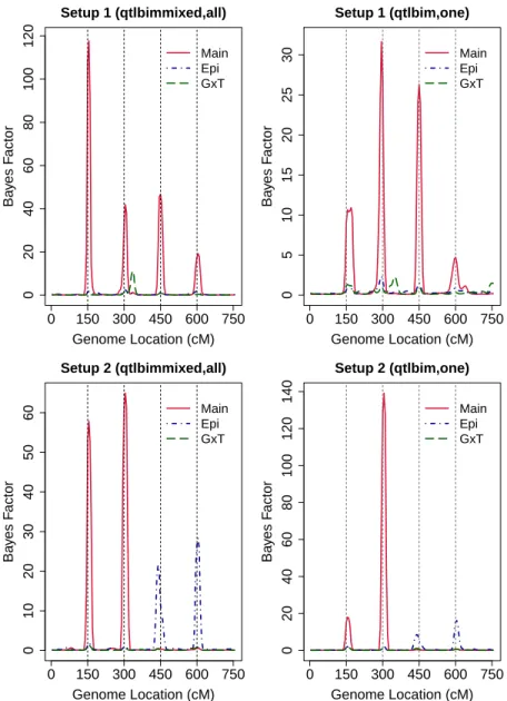
2.1 Estimated marginal Bayes factors for each marker from R/qtlbimmixed with all time points and R/qtlbim with one randomly selected time point for Setups 1 and 2. The solid (red), dot-dashed (blue) and long-dashed (green) lines represent main, epistatic effects and gene-time interaction, respectively. . . 58 2.2 Estimated marginal Bayes factors for each marker from R/qtlbimmixed

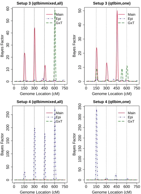
with all time points and R/qtlbim with one randomly selected time point for Setups 3 and 4. The solid (red), dot-dashed (blue) and long-dashed (green) lines represent main, epistatic effects and gene-time interaction, respectively. . . 59 2.3 Estimated ROC curves for Setups 1, 2, 3 and 4: solid line (red) - proposed

R/qtlbimmixed on all data; dot-dashed line (blue) - R/qtlbim on one randomly selected time point data; long-dashed lines (green) - R/qtlbim on all data. . . 60 2.4 Trace plots of σ2_,δ

1,δ2,δ3,ψ21,ψ31andψ32 for Setups 1,2,3 and 4 in the

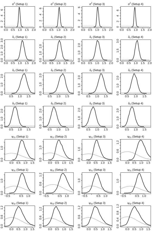
simulation study. The black lines represent the values of the draws for all parameters at each iteration and gray lines represent the true values of the parameters. . . 61 2.5 Posterior (solid line) and prior (dashed line) densities of the parameters

for random errors and random effects for Setups 1,2,3 and 4. Estimated densities are based on 10000 random draws. . . 62 2.6 95% HPD intervals of σ2_,δ

1,δ2,δ3,ψ21,ψ31and ψ32 for Setups 1,2,3 and

4. The blue dots represent the posterior means and blue lines represent HPD intervals. . . 63 2.7 Genomewide profile of Bayes factors for body weight in backcross mice

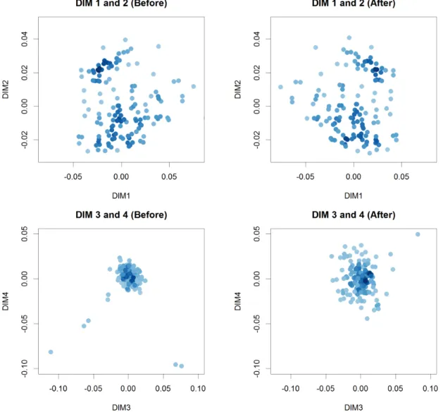
involving NZO/HILtJ and NON/ShiLtJ. The solid line (red) represents main effects, the dashed line (blue) represents epistasis effects and long-dashed line (green) represents gene-time interactions. . . 64 2.8 MDS plots for top four MDS scores from the genome-wide estimate of

2.9 Genomewide Manhattan plots of −log₁₀(P-value) for association with SBP and DBP measurements from extended EMMA, on the basis of covariance matrix estimated from SAS. Two dashed horizontal lines rep-resent the thresholds for suggestive (P-value=10−5_{) and significant}

(P-value=5×10−7) genomewide association. . . 66 2.10 Genomewide Manhattan plots of 2log(BF)for all combined effects with

SBP and DBP measurements from R/qtlbimmixed. Two dashed hori-zontal lines represent the genomewide thresholds for moderate (BF=10) strong (BF=30) genomewide associations. . . 67

3.1 Posterior mean estimates of the latent variableγgk andγtmfrom gpmixed

with all time points, original gp with one randomly selected time point and R/qtlbimmixed with all time points for Setups 1 and 2. . . 91 3.2 Posterior mean estimates of the latent variableγgk andγtmfrom gpmixed

with all time points, original gp with one randomly selected time point and R/qtlbimmixed with all time points for for Setups 3 and 4. . . 92 3.3 Estimated ROC curves for Setups 1,2,3 and 4: solid line (red) - proposed

gpmixed on all data; dot-dashed line (blue) - original gp on one randomly selected time point data; long-dashed lines (green) - R/qtlbimmixed on all data. . . 93 3.4 Trace plots of σ2_,δ

1,δ2,δ3,ψ21,ψ31andψ32 for Setups 1,2,3 and 4 in the

simulation study. The black lines represent the values of the draws for all parameters at each iteration and gray lines represents the true values of the parameters. . . 94 3.5 Posterior (solid line) and prior (dashed line) densities of the parameters

for random errors and random effects for Setups 1,2,3 and 4. . . 95 3.6 95% HPD intervals of σ2_,δ

1,δ2,δ3,ψ21,ψ31and ψ32 for Setups 1,2,3 and

4. The blue dots represent the posterior means and blue lines represent HPD intervals. . . 96 3.7 Genomewide profile of probability of being included in the model for

4.1 Posterior mean estimates of the latent variable γgk from the proposed

GP model and the original GP model for Setups 1 and 2 with common variants (cg1=0.30 andc_g2 =0.20). . . 112 4.2 Posterior mean estimates of the latent variable γgk from the proposed

GP model and the original GP model for Setups 3 and 4 with common variants (cg3=0.20 andc_g4 =0.20). . . 113 4.3 Posterior mean estimates of the latent variableγgk from the proposed GP

model and the original GP model for Setups 1 and 2 with rare variants (cg1 =2.50 and c_g2=1.00). . . 114 4.4 Posterior mean estimates of the latent variableγgk from the proposed GP

model and the original GP model for Setups 3 and 4 with rare variants (cg3 =2.00 and cg4=1.00). . . 115

4.5 Posterior mean estimates of the latent variableγgk from the proposed GP

model and the original GP model for Setups 1 and 2 with both common and rare variants (cg1=2.50 and c_g2=1.00). . . 116 4.6 Posterior mean estimates of the latent variableγgk from the proposed GP

model and the original GP model for Setups 3 and 4 with both common and rare variants (cg3=2.00 and c_g4=1.00). . . 117 4.7 Estimated ROC curves for Setups 1,2,3 and 4 where each group has

twenty common variants: solid line (red) - proposed GP model; dot-dashed line (blue) - original GP model. . . 118 4.8 Estimated ROC curves for Setups 1,2,3 and 4 where each group has

different number of common variants (10, 15, 20, 25 or 30): solid line (red) - proposed GP model; dot-dashed line (blue) - original GP model. . 119 4.9 Estimated ROC curves for Setups 1,2,3 and 4 where each group has

twenty rare variants: solid line (red) - proposed GP model; dot-dashed line (blue) - original GP model. . . 120 4.10 Estimated ROC curves for Setups 1,2,3 and 4 where each group has

different number of rare variants (10, 15, 20, 25 or 30): solid line (red) -proposed GP model; dot-dashed line (blue) - original GP model. . . 121 4.11 Estimated ROC curves for Setups 1,2,3 and 4 where each group has

LIST OF TABLES

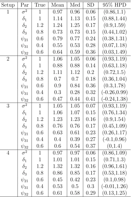
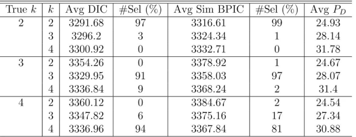
2.1 Posterior means, medians, standard deviations and 95% HPD intervals of the parameters for random errors and random effects in the simulation study. . . 68 2.2 Average DIC, average simplifed BPIC scores and percentage of selection

of the right number of true grids for Bayesian mixed effects model with different number of true grid points. . . 69 2.3 Genomewide association results for SBP,DBassociated SNPs with

P-value <5∗10−7 sorted by P-value via extended EMMA. . . 70 2.4 Genomewide association results for SBP,DBP-associated SNPs with 2log

(BF) >6.8 sorted by 2log(BF)of all combined effects via R/qtlbimmixed. 71

3.1 Posterior means, medians, standard deviations and 95% HPD intervals of the parameters for random errors and random effects in the simulation study. . . 98 3.2 Average DIC, average simplifed BPIC scores and percentage of selection

CHAPTER 1

INTRODUCTION

1.1 Statistical Methods for QTL Mapping

QTL Mapping

Single Gene Model

The basic quantitative genetic model partitions the total variance in quantitative traits into genetic variance and environmental variance. For individual i, Pi =G_i+E_i where Pi is phenotypic value, Gi is genetic value and Ei is environmental effect. Suppose

two inbred parents (P1 and P2) differ in some quantitative traits. At locus q, the allele of parent P1 is labeled as Bq and the allele of P2 as bq. An F1 generation is

completely heterozygous with genotype Bqbq, receiving one allele from each parent. A

BC population is generated when F1 is crossed back with P1 (or P2). At locusq, every BC individual has equal probability of 1/2 to beBqbqandBqBq(orbqbq). If the average

phenotypic value of P1 and P2 ism, the expected genetic values of Bqbq and BqBq (or

bqbq) can be defined as m+d_q and m+a_q (or m−a_q) whered_q is the dominance effect andaq is the additive effect. The genetic value for BC can be expressed asGi=µ+c_qx_iq whereµ=m+1

2(dq+aq)(or m+ 1

2(dq−aq)), andxiq =siq− 1

2 if siq denotes the number

of allele bq (or Bq). An F2 population is generated when F1 individuals are crossed

with each other and each F2 individual has probability of 1/4,1/2 and 1/4 to be bqbq,

Bqbq and BqBq, respectively. The expected genetic values of bqbq, Bqbq and BqBq can

be defined as m−a_q, m+d_q and m+a_q. The genetic value for F2 can be modeled as Gi=µ+e_qx_iq+f_qz_iq where µ=m+1₂d_q,x_iq =s_iq−1 and z_iq= (1+x_iq)(1−x_iq) −1₂ if s_iq denotes the number of allelebq.

Genetic Model for Epistasis

[1977], Haley et al. [1992] and Kearsey et al. [1998] applied theF_∞-metric model to study epistasis. Goodnight [2001] adopted an alternative model modified from Cockerham [1954] to the study of gene-gene interaction. Among them, Cockerham’s model is more appropriate than the other models for studying epistasis and mapping QTL in the populations, such as BC and F2 [Kao and Zeng, 2002]. For the commonly used Cockerham epistatic model, it is assumed that there are two alleles affecting the traits of interest. At two loci q and q′, the genotypes of P1 and P2 are BqBqBq′Bq′ and

bqbqbq′bq′, and all F1 individuals have genotype BqbqBq′bq′. Each BC population has

equal probability of 1/2 for beingBqbqBq′bq′ andBqBqBq′Bq′ (orbqbqbq′bq′). The genetic

values for BC can be expressed as Gi =µ+c_qx_iq+c_q′xiq′ +c_qq′xiqq′ where xiq =s_iq−1₂ and xiqq′ = x_iqx_iq′ if siq denotes the number of allele bq (or Bq). Each F2 individual

has probability of 1/4,1/2 and 1/4 for being bqbqbq′bq′, BqbqBq′bq′ and BqBqBq′Bq′,

respectively. The genetic value for F2 can be modeled asGi=µ+e_qx_iq+f_qz_iq+e_q′x_iq′+ fq′ziq′ +iaawiaa+i_adw_iad+i_daw_ida+i_ddw_idd where x_iq=s_iq−1,z_iq = (1+x_iq)(1−x_iq) −1₂, wiaa = x_iqx_iq′, w_iad = x_iqz_iq′, w_ida = z_iqx_iq′ and w_idd = z_iqz_iq′. In the above model, iaa, iad, ida and idd are the epistatic effects between loci q and q′, called additive × additive, additive × dominance, dominance × additive and dominance × dominance effects, respectively.

Single QTL Mapping

The QTL data include the phenotype valuesyi(i=1, ..., n), the marker genotype values Mij (i, ..., n, j=1, ..., m)located at certain positionsλ_j wherenis the sample size andm is the number of makers. The genotypes at a putative QTL are denoted by{qq, Qq, QQ} to distinguish the QTL genotypes from the marker genotypes {mm, M m, M M}.

QTL mapping become a simple linear regression problem. For BC population, the model can be specified as

yi=µ+βx_i+e_i (i=1, ..., n), (1.1)

whereµis the overall mean;β is the genetic effect;xi is 1/2 if individual i hasQq

geno-type and -1/2 if individual i hasQQgenotype; ei is a random error withei∼N(0, σ2). A test can be performed on β under H0 ∶β =0 vs H₁ ∶β ≠0. For F2 population, the model can be constructed to test additive and dominance effects separately as

yi=µ+βx_i+γz_i+e_i (i=1, ..., n), (1.2)

where β is the coefficient for additive effect; γ is the coefficient for dominance effect xi is 1 for qq, 0 for Qq and -1 for QQ; zi is 1/2 for Qq, -1/2 for qq and QQ. Linear

regression can be conducted to test H0 ∶ β =γ =0. If the effect of a marker is tested to be significant, that marker is claimed to be associated with one or more QTL. Although this single marker analysis is simple and captures candidate QTL, it cannot tell whether the markers are linked to one or more QTL and it does not estimate the putative positions of the QTL.

In practice, the QTL position is rarely known and the genotypes of QTL are usually unobserved, leading to all missing xis and zis. To solve this problem, interval

map-ping was introduced by Lander and Botstein [1989]. At any putative QTL position located in an interval between two flaking markers (Mij, Mij+1)of the individuali, the probabilities of the unobserved QTL genotypes (Qi) for each individual are computed

markers or between a marker and a putative QTL. The distribution of the quantita-tive trait given the flanking maker genotypes follows a finite mixture model and the likelihood functions for BC and F2 are given by

LBC(µ, β, σ2, λ) = n

∏

i=1

[PiQQφ((yi−µ+ 1

2β)/σ) +PiQqφ((yi−µ− 1

2β)/σ)], (1.3)

LF2(µ, β, γ, σ2, λ) =

n ∏ i=1

[P_iQQφ((y_i−µ+β+ 1

2γ)/σ)+PiQqφ((yi−µ−

1

2γ)/σ)+Piqqφ((yi−µ−β+

1

2γ)/σ)],

respectively, whereφ(z)is the standard normal density function. The above likelihood functions can be maximized using EM algorithm to obtain MLE estimates (ˆµ,β,ˆ γ,ˆ σˆ2_).

Since the genotypes of QTL are treated as the missings, the observed data include only phenotypes and maker genotypes while the full data include phenotypes, marker genotypes and QTL genotypes. Test statistics are constructed using the LOD scores

LODBC(λ) =log10

LBC(ˆµ,β,ˆ σˆ2) LBC(˜µ,0,σ˜2)

, LODF2(λ) =log10

LF2(ˆµ,β,ˆ ˆγ,σˆ2) LF2(˜µ,0,0,σ˜2)

, (1.4)

where ˜µ and ˜σ2 _{are MLE estimates under the null hypothesis H}

procedure.

Multiple Interval Mapping

If there exist more than one QTL affecting the trait on the chromosome, single QTL method may fail to discover true QTL and instead identify ghost (false) QTL. Moreover, single QTL model may fail to detect QTL with high epistatic effect but low marginal effect. To solve this problem, multiple interval mapping [Kao and Zeng, 1997; Kao et al., 1999] was proposed. This method combines QTL mapping with the analysis of genetic architecture of quantitative traits through a search algorithm to search for the number and position of QTL and their genetic effects. Suppose there are p putative QTL and t significant pairwise epistatic effects. Note that the model only contains a subset (t pairs) of QTL pairs that each shows a significant epistatic effect since if all pairs of p QTL are fitted in the model, it can be overparameterized. Cockerham’s genetic model is used to define the genetic parameters. The main advantage of Cockerham’s model is that it has an orthogonal property in modeling genetic effects. For BC population, the model of multiple interval mapping can be expressed as

yi =µ+

p

∑

r=1

βrxir+

t

∑

r≠s

βrsxirxis+e_i=µ+x_iβ+e_i, (1.5)

where βr, βrs are the marginal and epistatic effect; xir is 1/2 for Qq and -1/2 for QQ; β is the(p+t) ×1 vector of marginal and epistatic effects; x_i is the 1× (p+t) vector of indicator variables. For F2 population, the model is given by

yi =µ+

p

∑

r=1

(βrxir+γ_rz_ir) +

t

∑

r≠s

xir is 1 for qq, 0 for Qq, -1 for QQ and zir is 1/2 for Qq, -1/2 for QQ and qq; γ is

the (2p+4t) ×1 vector of all effects;z_i is the 1× (2p+4t) vector of indicator variables. Even though the genotype of each putative QTL (Qij) in intervalIij is unobserved, the

probabilities ofQij can be inferred from the flanking markers ofIij based on the

recom-bination frequency between them. We have P(Qi1, ..., Qip∣Ii1, .., Iip) = ∏p_j=1P(Qij∣Iij).

We refer Pij (j = 1, ...,2p for BC, j =1, ...,3p for F2) as the conditional probabilities of all possible QTL genotypes of individuali. The likelihood functions of the multiple interval mapping for BC and F2 are the following mixture of normal distributions:

LBC(β, µ, σ2) =

n

∏

i=1

[

2p

∑

j=1

Pijφ(

yi−µ−x_ijβ

σ )], LF2(γ, µ, σ

2

) =

n

∏

i=1

[

3p

∑

j=1

Pijφ(

yi−µ−z_ijγ σ )],

(1.7) where φ(z) is the standard normal density function. Again, for the MLE estimates of (β,γ, µ, σ2_{), EM algorithm can be employed. The test for marginal effect is performed}

by LOD score for H0 ∶ βr = 0 or H0 ∶ γr = 0. For testing epistatic effect, we use

LOD score for βrs = 0, δ_rs = 0, ξ_rs = 0 and γ_rs = 0. In theory, multiple interval mapping can be applied to more than two QTL straightforwardly. However, since the search becomes multidimensional, there are some difficulties in parameter estimation and model identifiability to map more than two QTL simultaneously in practice.

Bayesian Interval Mapping

Several Bayesian methods for QTL mapping has been proposed. Satagopan et al. [1996] proposed a Bayesian methods to detect multiple QTL simultaneously using Markov chain Monte Carlo (MCMC) method. When the quantitative trait is explained by multiple genes (p genes) acting independently and their interactions, we have

yi =µ+

p

∑

j=1

βjxij+

t

∑

j≠k

wherexiis thepQTL genotypes and their interactions for theith individual andβis the

marginal and epistatic effects of theploci. The genetic parameters are model unknowns (β,µ,σ2_{) and the QTL loci λ = {λ}

j}p_j=1. For individual i, marker genotype M_i = {Mik}m_k=1 and phenotypic trait y= (y₁, ..., y_n)T are observed, but the genotypes of the putative QTL,xi are not observed. However, the conditional distributionP(x_i∣λ,M_i) can be obtained using recombination frequency between the putative QTL and the markers.

To implement Bayesian analysis, the prior distribution is required over the param-eter space (λ,β,µ,σ2_{). We assume prior independence of the parameters. That is,}

P(λ,β, µ, σ2) =P(λ)P(µ)P(σ2) ∏p_j=1βj∏t_j≠kβjk. A natural choice of prior for λwhen

there is no available information regarding the location would be a uniform distribu-tion for p ordered variables on [0,Dm] where Dm is the length of the linkage group

(0<λ₁<...<λ_p<D_m). The prior for overall meanµ is a normal distribution centered at 0 with variance τ2

µ (µ∼N(0, τµ2)). The phenotypic variance σ2 is assumed to have

an inverse gamma prior (σ2

∼IG(u, v)). The priors of QTL effectβ_j,β_jk (j, k=1, ..., p) are independent normal distributions with mean 0 and varianceτ2

β (βj, βjk ∼N(0, τβ2)).

The posterior distribution over all the unknown parameters (λ,β,µ,σ2_{) is given}

where λ₋j represents all the elements of λ except λj. For model unknown

parame-ters, we can directly sample β, µ and σ2 _{from their full conditionals. The full}

condi-tionals are given by βj∣λ,β_−j, µ, σ2,y∼N(η_βj, τ_β2

j), βjk∣λ,β−jk, µ, σ

2_,y∼N(η βjk, τ

2 βjk),

µ∣λ,β, σ2_,y∼N(η

µ∗, τ_µ2∗) and σ2∣λ,β, µ,y∼IG(u_σ2, v_σ2) (see Satagopan et al. [1996] for more details). The marginal posterior density ofβ,µandσ2 _{can be estimated since}

their full conditional densities are known completely. However, since the full condi-tional density of λ is not known, the density estimates of λ should be obtained from the MCMC samples by different kernel estimate methods (for example, the histogram estimator). Confidence intervals can be obtained as high posterior density (HPD) re-gions.

1.2 Gaussian Process Models

Bayesian Neural Networks

regression than other nonlinear models [Rasmussen, 1996].

The idea of using Gaussian process directly came from investigations by Neal [1996] into prior over weights for neural networks [Rasmussen, 1996]. We consider a neural network with J inputs, one layer of K tanh hidden units and one output unit. Both hidden and output units have weights and biases and the network is fully connected between consecutive layers:

ψk(x) =tanh(

J

∑

j=1

ujkxj+u₀), η(x) =

K

∑

k=1

vkψk(x) +v₀. (1.9)

The zero mean Gaussian priors are imposed on all weights and biases. That is, ujk ∼ N(0, σ_u2), u₀ ∼ N(0, σ_u02 ), v_k ∼ N(0, σ_v2) and v₀ ∼ N(0, σ2_v0). Given a specific input vector xi, we can derive the distribution of a output based on the priors on

weights and biases. We have E[v_kψ_k(x_i)] = E[v_k]E[ψ_k(x_i)] = 0 (∵ v_k–ψ_k(x_i)) and E[(v_kψ_k(x_i))2] = σ2_vE[(ψ_k(x_i))2] (∵ ψ_k(x_i) is bounded). By Central Limit Theo-rem (CLT), as the number of hidden units K goes to infinity, the prior distribu-tion of η(xi) converges to a Gaussian distribution with mean 0, variance c(x_i) = σ2

v0 +Kσv2E[(ψk(x_i))2]. If we choose σ2_v which scales inversely with K, a well de-fined prior can be obtained in the limit of infinite number of hidden units. Using the similar argument, the joint distribution for multiple inputs converges in the limit ofK to a multivariate Gaussian with mean 0 and covariance c(x_i,x_i′) = E[η(x_i)η(x_i′)] = σ2

v0+Kσv2E[ψk(x_i)ψ_k(x_i′)].

Gaussian Process Models

a collection of random variables {η_x} indexed by a set x∈X, where any finite subset of ηx’s has a joint multivariate Gaussian distribution. Often, Gaussian processes are

defined over time, where the index set is time, but in our case, we index the random variables η= {ηx}by the input space X.

Consider the case where a training set of n observations is available and thus data set D = {(x_i, y_i)∣i = 1, ..., n} = {x,y}, where x_i is a vector of p covariates and y_i is the scalar response. We will consider the following Bayesian regression model with Gaussian noise

yi =η(x_i) +e_i (i=1, ..., n), (1.10)

whereηis an unknown function ofpcovariates that we modeled via a Gaussian process prior and ei is a noise with distribution N(0, σ2e).

The Gaussian process is completely specified by its mean function m(xi) and co-variance functionc(xi,xi′). The Gaussian process can be expressed asη∼ G P (m(xi),

c(xi,xi′)). From here on, we will consider only Gaussian process model with a mean

of zero, such thatη∼ G P (0, c(xi,xi′)). One of examples of a covariance function is

c(xi,xi′) =a₀+a₁

p

∑

k=1

xikxi′k+v₀exp(− 1 2

p

∑

k=1

wk(xik−x_i′k)2), (1.11)

where xi = (xi1, ..., xip) and a₀, a₁, v₀, w₁, ..., w_p are hyperparameters. In this function, first two terms involving a0 anda1 control the scale of the bias and linear contribution

to the covariance. The contribution from the linear terms in the covariance function may become large for inputs which are quite distant from the bulk of the output values. The exponential part defines the correlation between outputs and nearby inputs. The parameter wk is multiplied by the coordinate-wise distance in input space and thus

parameter wk get large for relevant inputs. The parameter v0 defines the overall scale

of the local correlations. The functions of Gaussian process are smooth and stationary. These are properties which are induced by the covariance function. In the Gaussian process models, the role of the kernel function and local model are both integrated in the covariance function. Like the kernel function, the covariance function is a function of the model inputs, it returns the covariance between the output corresponding to two inputs. The problem of learning in Gaussian processes is exactly the problem of finding suitable properties of the covariance function.

Marginal Likelihood

Letθ= (a₀, a₁, v₀, w₁, ..., w_p, σ2_e),η_i=η(x_i)andη= (η₁, ..., η_n)such thatη∼ G P (0,Σ_η). By the independence assumption, we have the likelihood asP(y∣η,θ) = ∏_in₌₁P(yi∣ηi,θ)

d

=N(η, σ2_eI_n). The marginal likelihood of y, P(y∣θ)is given by

P(y∣θ_{) = ∫} P(y∣η,θ)P(η)dη=dN(0,Σ) where Σ=Σ_η+σ_e2I_n. (1.12)

The term marginal likelihood refers to the marginalization over the function value η. The log likelihood of the hyperparameters and its partial derivatives are given by

logP(y∣θ) = − 1

2log∣Σ∣ − 1 2y

T_Σ−1

y−

n 2log2π, ∂

∂θi

logP(y∣θ) = −1 2tr(Σ

−1∂Σ

∂θi

) +1 2y

T_Σ−1∂Σ

∂θi

Σ−1y. (1.13)

Prior Specification

Letτa0 =1/a0, τa1 =1/a1, τv0 =1/v0, τe =1/σ

2

e. We impose the Gamma priors on these

four parameters: τa0 ∼Ga(

αa0

2 , αa0

2µa0), τa1

∼Ga(α₂a1,_2µαa1

a0), τv0

∼Ga(α₂v0,_2µαv0

v0

) and τ_e ∼ Ga(αe

2 , αe

2µe)whereαa0, αa1, αv0, αeare positive shape parameters andµa0, µa1, µv0, µeare

the means of τa0, τa1, τv0, τe. The large values of α’s produce priors concentrated near

µα’s. The priors for hyperparameter wi are more complicated. As we expect the prior

on the importance of hyperparameterwi to be lower with increasing numbers of input

(i.e. large p), we let τwi = 1/wi and put a gamma prior whose mean scales with the

number of inputs p on τwi as τwi ∼Ga( α_wi

2 , α_wi

2µ_wi) where µwi =µ0p

2/α_{wi. Large p makes}

µwi large and the mean of wi small.

Hybrid Monte Carlo Method

The joint posterior distribution marginalized with respect to η is computed from the marginal likelihood multiplied by the prior: P(θ∣y) ∝ P(y∣θ)P(θ). To obtain the posterior distribution, we need to integrate over the resulting posterior, but analytic integration is infeasible due to the complex form of the likelihood. The Hybrid Monte Carlo method [Duane et al., 1987] is appropriate for this case. When sampling from complicated multidimensional distributions, it is often advantageous to use gradient information to find regions of high probability when gradients can be obtained. The Hybrid Monte Carlo method avoids the random walk behavior by creating a virtual dynamic system where hyperparameter θ plays the role of position variables, which are augmented by a set of momentum variables φ. The kinetic energy is a function of momentum variables: K(φ) = 1

2∑ p+4

i=1 φ2i where φ = (φ1, ..., φp+4) is in one-to-one

K(φ) + E (θ). The dynamical system evolved through virtual timet is governed by the following Hamilton’s differential equations:

dθi

dt = ∂H ∂φi

=φ_i,

dφi

dt = − ∂H ∂θi

= − ∂E ∂θi

. (1.14)

Since the partial derivative ofE with respect to θ is a complicated function, the above equation cannot be simulated exactly. We use the following leapfrog steps to approxi-mate the dynamic system:

φi(t+

2) =φi(t) − 2

∂E ∂θi

(θ(t)), (1.15)

θi(t+) =θ_i(t) +φ_i(t+ 2), φi(t+) =φ_i(t+

2) −

2

∂E ∂θi

(θ(t+)),

where is the step size for discretizing the dynamic system. The step size is set to the same value for all hyperparameters and is chosen to∝n−1/2 since the magnitude of the gradients under the posterior are expected to be scale roughly as n1/2 _{when the}

prior is vague. Rasmussen [1996] found that =0.5n−1/2 performs reasonably well, in practice.

Maximum a Posteriori (MAP) Estimates

et al., 2003] and sparse grid approximation [Bungartz and Griebel, 2004] can be used [Hegland, 2007].

1.3 Bayesian Model Selection Methods

Bayesian Model Selection

A Bayesian approach to model selection is concerned with the following situation [Han and Carlin, 2001]. Suppose the observed datay are considered to have been generated by a model m∈ M, where M is the finite set of competing models. Corresponding to model m, there is a distinct unknown parameter vector θm∈Θ_m of dimension pwhere Θm is the set of all possible values for θm. Each model specifies the distribution of y, P(y∣m,θ_m). If P(m) is the prior probability of model m, where ∑_m∈MP(m) = 1, the posterior probability is given by P(m∣y) = P(m)P(y∣m)

∑m∈MP(m)P(y∣m), m

∈ M where P(y∣m) is the marginal likelihood computed from P(y∣m_{) = ∫} P(y∣m,θ_m)P(θ_m∣m)dθ_m and P(θ_m∣m)is the model-specific conditional prior of θ_m. To compare two models,m and m′, we often use the Bayes factor for model m overm′:

BFmm′ =

P(m∣y)/P(m) P(m′∣y)/P(m′)

=

P(y∣m) P(y∣m′)

. (1.16)

The Bayes factor BFmm′ captures the change in the odds in favor of model m as

model and subsequently calculate the Bayes factor using equation (1.16). Chen and Shao [1998] developed an importance sampling approach to estimate the marginal likeli-hood using a technique of Chen and Shao [1997]. Newton and Raftery [1994] proposed the estimator for marginal likelihood, which is the harmonic mean of the likelihood values sampled from the stationary phase of the MCMC run. Chib [1995] and Chib and Jeliazkov [2001] provides a indirect method to estimate marginal likelihood in the context of Gibbs sampling and Metropolis-Hastings algorithm. All methods operate on a posterior sample that has already been produced by some noniterative or MCMC method, although the methods of Chib [1995] and Chib and Jeliazkov [2001] will often require multiple runs of slightly different version of the MCMC algorithm to produce the necessary output. However, for some complicated or high-dimensional models, these approaches are difficult to implement.

A slight more direct and more common approach to estimating posterior model probabilities using MCMC is to include the model indicator γ as a parameter in the sampling algorithm. This may complicate the initial sampling process, but has the clear benefit of producing a stream of samples{γ_i}H_i=1from the marginal posterior distribution of the model indicator, P(γ∣y). Once the sampler converges, the proportion of times the sampler visits modelm is a simple estimate of each posterior model probability:

P(γ=m∣y) =

number of γi =m ∑H_i=1number of γi

,m=1, ..., K. (1.17)

This estimate can be used to compute the Bayes factor between any two of the models, say m and m′:

BFmm′ =

P(γ=m∣y)/P(γ =m) P(γ =m′∣y)/P(γ =m′)

. (1.18)

a sampler that operates over the model space alone. Unfortunately, most model settings are too complicated to allow the entire parameter θ to be integrated out of the model in a closed form, and thus require that the MCMC search be over the model and parameter space jointly. This joint search approach also permits posterior estimate of the parameters under each modelP(θ∣γ =m,y), simply by conditioning on the samples produced when the chain is currently in state γ=m.

Stochastic Search Variable Selection

George and McCulloch [1993] proposed a model selection procedure which is called stochastic search variable selection (SSVS). This method introduces latent variables to determine whether particular regression coefficients may safely be estimated by 0 or not. We consider the following simple linear model

y=xβ+e, e∼N(0, σ2I), (1.19)

wherey= (y₁, ..., y_n)T isn×1, x= (x₁, ...,x_p) isn×p,β= (β₁, ..., β_p)T isp×1 and eis n×1. We assign prior for each β_i to be a mixture of two normal densities,

βi∣γi∼ (1−γ_i)N(0, τ_i2) +γ_iN(0, c2_iτ_i2), (1.20)

whereγi(i=1, ..., p)is a binary variable withP(γ_i=1) =1−P(γ_i=0) =p_i. Whenγ_i =0, βi∼N(0, τ_i2)and whenγ_i=1,β_i ∼N(0, c2_iτ_i2). Whenτ_i(τ_i>0)is small andγ_i =0, then βi would probably be small that it could safely be estimated by 0. Whenci (ci >1)is large andγi=1, then a non-zero estimate ofβ_i is probably included in the final model. Based on this interpretation,pi can be viewed as a prior probability thatβi is non-zero.

The mixture prior forβi∣γi can be written in vector form asβ∣γ∼N(0,D_γRD_γ)where

ai =1 if γi =0 and ai =ci if γi =1. We use the inverse gamma conjugate prior as the

prior for σ2_{: σ}2_∣γ∼IG(νγ 2 ,

νγλγ

2 ) whereνγ and λγ are hyperparameters to be specified.

Product Space Search

Carlin and Chib [1995] proposed a Gibbs sampling method that avoids convergence difficulties and accommodates fairly general model settings. Suppose there areK can-didate models, a distinct parameter vector θm (m = 1, ..., K) for each model, whose prior is assumed to be independent each other given the model indicator γ. Corre-sponding to model m, the likelihood is P(y∣θ_m, γ=m) and the prior is P(θ_m∣γ =m). Since γ is an indicator of which θm is relevant to y, y is independent of θ−m given

the model indicator γ where θ₋m represents all elements of θ except θm. Under the

conditional independence assumption, we have

P(y∣γ=m) = _∫ P(y∣θ_m, γ=m)P(θ∣γ=m)dθ

= _∫ P(y∣θ_m, γ=m)P(θ_m∣γ=m)dθ_m, (1.21)

which has nothing to do with the pseudoprior P(θ_m∣γ ≠m). Therefore, a pseudoprior is only conveniently chosen liking density which is used to completely define the joint model specification. In order to implement the Gibbs sampler, the full conditional distribution ofθm is given by

P(θ_m∣θ_−m, γ,y) ∝ ⎧ ⎪ ⎪ ⎪ ⎪ ⎨ ⎪ ⎪ ⎪ ⎪ ⎩

P(y∣θ_m, γ=m)P(θ_m∣γ=m) if γ =m P(θ_m∣γ≠m) if γ ≠m

(1.22)

pseudoprior. The full conditional distribution of the model indicator γ is given by

P(γ=m∣θ,y) =

P(y∣θ_m, γ=m)[∏_m′_∈MP(θ_m′∣γ=m)]P(γ=m) ∑K_k=1{P(y∣θ_k, γ=k)[∏_m′_∈MP(θ_m′∣γ =k)]P(γ=k)}

. (1.23)

Under the usual regularity conditions [Smith and Roberts, 1993], this Gibbs sampler will produce posterior samples from all conditional posterior distributions. When the Gibbs sampler converges, the posterior probability of model m can be estimated by

P(γ =m∣y) = 1 H

H

∑

i=1

I(γi=m), (1.24)

which can be used to estimate the Bayes factors in favor of model m as

BFmm′ =

P(γ=m∣y)/P(γ =m) P(γ =m′∣y)/P(γ =m′)

. (1.25)

Dellaportas et al. [2002] proposed a hybrid Gibbs-Metropolis version of product space search method. In this method, the model selection step is based on a proposal for a move from model m to m′ with acceptance rate αmm′. This method is called

Metropolized product space search method which proceeds as follows [Han and Carlin, 2001]: (1) Let the current state be (m,θm), where θm is of dimension pm. (2)

Pro-pose a new modelm′ with probability h(m, m′). (3) Generate θ_m′ from a pseudoprior P(θ_m′∣γ≠m′)as in product space search method. (4) Accept the proposed move from model m to model m′ with acceptance rate

αmm′ =min{1,P

(y∣θ_m′, γ=m′)P(θ_m′∣γ=m′)P(θ_m∣γ=m′)P(γ =m′)h(m′, m)

P(y∣θ_m, γ=m)P(θ_m∣γ =m)P(θ_m′∣γ=m)P(γ=m)h(m, m′)

}. (1.26)

Reversible Jump MCMC

As the product space search method, the reversible jump MCMC method originally proposed by Green [1995], samples over the model and parameter space jointly but it avoids the full product space search at the cost of a less straightforward algorithm operating on the union space,M × ⋃m∈MΘm. This method generates a Markov chain

that can jump between models with different dimensional parameter spaces, while re-taining the aperiodicity, irreducibility, and detailed balance conditions necessary for MCMC convergence. The reversible jump MCMC algorithm proceeds as follows [Han and Carlin, 2001]: (1) Let the current state be (m,θm), where θm is of dimension pm.

(2) Propose a new modelm′ with probabilityh(m, m′). (3) Generateufrom a proposal densityq(u∣θ_m, m, m′). (4) Set(θ_m′,u′) =g_m,m′(θ_m,u), where g_m,m′ is a deterministic function that is one-to-one and onto. This is a dimension-matching function, specified so thatpm+dim(u) =p_m′+dim(u′). (5) Accept the proposed move from modelm to model m′ with the acceptance rate

αmm′=min{1,

P(y∣θm′, γ=m′)P(θm′∣γ=m′)P(γ=m′)h(m′, m)q(u′∣θm′, m′, m)

P(y∣θ_m, γ=m)P(θ_m∣γ=m)P(γ=m)h(m, m′_)q(u∣θ

m, m, m′) ∣

∂g(θm,u)

∂(θ_m,u) ∣}.

(1.27)

When m′ = m, the move can be either a standard Metropolis-Hastings or a Gibbs step. Posterior model probabilities and Bayes factors can be computed as described earlier. The dimension-matching aspect of this algorithm is a little obscure, so that further discussion is needed. Suppose we are comparing two models, for whichθm ∈ R1 and θm′ ∈ R2 and θ_m is subvector of θ_m′. If we consider moving from model m to model m′, we simply drawu∼q(u) and setθ_m′ = (θm, u). In this case, the

dimension-matching functiongis identity function andu′should be ignored. We can seth(m, m) = h(m, m′) =h(m′, m) =h(m′, m′) = 1₂ and the Jacobian of step 5 is equal to 1.

Composite Model Space Framework

are allowed to be shared between different models. If a standard Gibbs sampler is applied to this composite model space, it becomes the product space search method. However, a more sophisticated Metropolis-Hastings algorithm approach produces a version of the reversible jump algorithm that avoids the dimension matching step. The composite model space procedure is applicable when there exists a subvectorβ_m′ of the parameter vectorθm′ for the modelm′ such thatP(θ_m′∣θ_m′_(−β

m′), γ=m′,y)is available

in closed form, and in the current modelm, there exists an equivalent subvectorθm(−βm)

of the same dimension as θm′(−βm′). The composite model space algorithm proceeds

as follows [Han and Carlin, 2001]: (1) Let the current state be (m,θ_m), where θ_m is of dimension pm. (2) Propose a new model m′ with probability h(m, m′). (3) Set θm(−βm)=θm′(−βm′). (4) Accept the proposed move with the acceptance rate

αmm′ =min{1,

P(m′∣θ_m′₍₋β_m′),y)h(m′, m) P(m∣θm(−βm),y)h(m, m′)

}, (1.28)

where P(m∣θm(−β_m),y) = ∫ P(m,βm∣θm(−β_m),y)dβm. (5) If the model move is

ac-cepted, update the parameters of the new model β_m′ and θm′(−β_m′) using standard Gibbs or Metropolis-Hasting steps; otherwise, update the parameters of the old model

β_m and θm(−βm) using standard Gibbs or Metropolis-Hastings steps. Note that model

move proposals from model m to model m always have acceptance rate 1, and thus when the current model is proposed, this algorithm could simplify to standard Gibbs or Metropolis-Hastings steps. Posterior model probabilities and Bayes factors can be computed as described earlier.

Variable selection is a special case of model selection. For variable selection, a natural parameterization for γ is as binary p-vector which is γ = {γ1, ..., γp} ∈ {0,1}p.

Deviance Information Criterion (DIC)

Suppose thaty= (y1, ..., yn)T is a vector ofn observations generated from an unknown distribution F(y) and a family of distributions with densities {P(y∣θ)∣θ∈Θ⊂Rp}is used to approximate the true distribution F(y). The prior density and the posterior density are P(θ) and P(θ∣y), respectively. The predictive distribution for a future observation z is defined asP(z∣y_{) = ∫} P(z∣θ)P(θ∣y)dθ.

To measure the deviation of the predictive distributionP(z∣y)from the true model P(z), Spiegelhalter et al. [2002] considered the following posterior mean of the expected loglikelihood,

ξ=E_z[E_θ∣y{logP(z∣θ_{)}] = ∫ {∫} logP(z∣θ)P(θ∣y)dθ}dF(z) (1.29)

[Ando, 2007]. A natural estimator of ξ is as follows:

ˆ ξ=

1

nEθ∣y{logP(y∣θ)} = 1

n∫ logP(y∣θ)P(θ∣y)dθ. (1.30)

The estimator ofξ, ˆξ, is generally positively biased since the same datay is used twice, one for constructing the posterior distribution P(θ∣y) and one for evaluating ξ. Note the expected bias of ˆξ is

bθ=E_y(ξˆ−ξ_{) = ∫ (}ξˆ−ξ)dF(y). (1.31)

Let ˆbθ be an estimator of bθ, then the bias-corrected estimator of ξ can be expressed

as 1_nEθ∣y{logP(y∣θ)} −bˆ_θ. Under this framework, Spiegelhalter et al. [2002] proposed the deviance information criterion (DIC),

where PD is an effective number of parameters, defined as PD = 2logP(y∣¯θ) −2Eθ∣y

{logP(y∣θ)}where ¯θ is the posterior mean ofθ.

Bayesian Predictive Information Criterion (BPIC)

Alternatively, Ando [2007] evaluated the asymptotic bias of ˆξand proposed the Bayesian predictive information criterion:

BP IC= −2Eθ∣y{logP(y∣θ)} +2nbˆ_θ, (1.33)

where ˆbθ =E[log{P(y∣θ)P(θ)}]−log{P(y∣θˆ_n)P(θˆ_n)}+tr{J_n−1(θˆ_n)I_n(θˆ_n)}+p/2,pis the dimension ofθ, ˆθn=argmax_θP(θ∣y)is the posterior mode and the matricesI_n(θˆ_n)and J−1

n (θˆn) are given by I_n(θˆ_n) = _n1 ∑_in₌₁{∂ξn_∂θ(yi,θ)∂ξn(yi,θ)

∂θT }, J− 1

n (θˆn) = −1_n∑_i=1{∂

2_ξ

n(yi,θ)

∂θ∂θT },

respectively. Here,ξn(y_i,θ) =logP(y_i∣θ) +logP(θ)/n. Further, Ando [2011] proposed a simplified version of BPIC as

Simplified BP IC1 = −2Eθ∣y{logP(y∣θ)} +2P_D, (1.34)

wherePD =nbˆ_θ=2logP(y∣θ¯_n)−2E_θ∣y{logP(y∣θ)}. If we impose additional assumptions that (a) the prior is assumed to be dominated by the likelihood as n increases, that is, logP(θ) =O(1), and (b) the specified models include the true model [Ando, 2011], then the estimated bias term nbˆθ reduces to nbˆθ ≈p and the BPIC can be further reduced to

1.4 Bayesian Covariance Estimation

Bayesian Mixed Effects Models

The most common model for repeated measurements is the linear mixed effects model of Laird and Ware [1982]. For individual i with ni repeated measurements, the mixed

effects model is given by

y_i=µ_i+x_iβ+z_ib_i+e_i, i=1,...,n, (1.36)

where y_i is an ni×1 response vector; µ_i is the overall mean vector; x_i is an n_i×p matrix of fixed covariates; β is a p×1 vector of fixed effects; z_i is an n_i×k matrix of random covariates;bi is ak×1 vector of random effects; ei is anni×1 vector of random

errors. It is standard to assumebi and ei are independent of each other and both are

normally distributed with bi ∼N(0,D) and e_i ∼N(0, σ2I_ni). Under this assumption,

y_i∣µ_i,β,D, σ2∼N(µ_i+x_iβ+z_ib_i, σ2I_ni). For Bayesian analysis of the random effects model [Zeger and Karim, 1991; Gilks et al., 1993], we specify the priors on µ_i, β, D

andσ2 _{traditionally, as the prior for µis chosen to be P(µ)=}d_N(µ

0, σ2µ), the prior forβ

is chosen to beP(β)=dN(0,Σ_β)and the prior for σ2 is chosen to be P(σ2)=dIG(δ₂0,γ₂0). By far the most common approach to the prior onDis to use an inverse-Wishart prior, motivated by its conjugacy property. That is,P(D)=dIW(n₀,C₀). However, there are many other choices of prior on the covariance D.

The usual inverse-Wishart prior is often inadequate because it is of restrictive form due to the common degrees of freedom for all the diagonal entries ofD. It is helpful to break the covariance matrix down into several components. There are several methods based on well-known matrix decompositions. Barnard et al. [2000] worked with the variance-correlation decomposition of the covariance matrix. Boik [2002] proposed a spectral decomposition on the matrix. Another approach is to use the Cholesky decomposition of the covariance matrix [Pourahmadi, 1999; Chen and Dunson, 2003].

Inverse Wishart Prior

Suppose A is a p×p positive definite random matrix. The Wishart distribution with n0 degree of freedom is characterized by A∼W(n₀,C−₀1) if and only if A= ∑n_i=0₁zizT_i ,

where p dimensional vectorsz1, ...,zn are i.i.d. random samples from N(0,C−01). The

diagonal elements of a Wishart matrix A are chi-square random variables. That is, aii ∼ σ_iiχ2_n, where a_ii is the ith diagonal element of A and σ_ii is the ith diago-nal element of C−₀1. If D = A−1, D have an inverse Wishart distribution, denoted by D ∼ IW(n₀,C₀). The mean of inverse Wishart distribution is E(D) = _nC0

0−p−1,

which means large n0 makes the prior relatively noninformative. Based on the inverse

Variance-Correlation Decomposition

The covariance matrixDcan be decomposed asD=SRSwhereSis thek×kdiagonal matrix of standard deviations and R is the k×k correlation matrix [Barnard et al., 2000]. This decomposition has a strong practical appeal since these two factors of D

are easily interpreted in terms of standard deviations and correlations. We can write the prior on D in terms of (S,R) as P(S,R) = P(S)P(R∣S). Since S only have k-dimensional elements with component-wise nonnegativity as the only constraint, we can specify the prior for S as P(log(s))=dN(ψ,Λ) where s= (s₁, ..., s_n) are diagonal elements of S and log(s) = (log(s1), ..., log(sn)). The choice of prior for R given S is

more complicated due to the complexity of space of correlation matrices, and often a marginally uniform prior or jointly uniform prior are used forR[Barnard et al., 2000].

Spectral Decomposition

The spectral decomposition of a covariance matrix D is given by D = PΛPT = ∑q_i=1λieieT_i , whereΛ is a diagonal matrix of eigenvalues with theith elementλi andP

is the orthogonal matrix of normalized eigenvectors with the ith column, ei

[Pourah-madi, 2011]. There are three classes of priors on Λ and P and details can be found in [Leonard and Hsu, 1992; Yang and Berger, 1994; Daniels and Kass, 1999].

Cholesky Decomposition

The standard Cholesky decomposition of a positive-definite matrix is given by D =

modified Cholesky decomposition

D=L∆−1∆∆∆−1LT =Ψ∆2ΨT, (1.37)

where Ψ = L∆−1. Chen and Dunson [2003] presented another modified Cholesky decomposition as follows.

D=∆∆−1LLT∆−1∆=∆ΨΨT∆, (1.38)

where Ψ=∆−1Lis obtained from L by dividing the elements of its ith row by δ_i. In this decomposition, ∆ is a diagonal matrix with elements proportional to the square roots of the diagonal elements ofD and Ψis a unit lower-triangular matrix solely de-termining its correlation matrix. This total separation of variance and correlation is one of advantages over the more traditional modified Cholesky decomposition of Pourah-madi [1999] [PourahPourah-madi, 2007]. Given Chen and Dunson [2003]’s decomposition, the reparameterized mixed effects model can be written as

y_i =µ_i+x_iβ+z_i∆Ψc_i+e_i, i=1,...,n, (1.39)

zero on the elements ofψ corresponding to zero∆. For ∆, we assume that the δ’s are independent of each other, so that P(∆) = Πk_l=1P(δ_l). Let ZI −N+(π, µ, σ2) denote the density of a zero inflated half normal distribution comprised of a point mass at zero with probability π and a N(µ, σ2_{) density truncated below by zero. The prior}

distribution for ∆ is given by P(∆) = Πk

l=1P(δl) = Π k

l=1ZI−N+(δl∣pl0, ml0, s 2

l0) where

pl0,ml0 and s2_l0 are hyperparameters to be specified.

1.5 Outline of Thesis

CHAPTER 2

BAYESIAN MULTIPLE QTL MAPPING FOR LONGITUDINAL TRAITS

2.1 Introduction

Many complex traits, such as blood pressure, cholesterol level are time-dependent or longitudinal traits and are affected by genetic factors as well as nongenetic factors (e.g. age, sex or drug). It is crucial to consider the repeated measurements of traits for better understanding their genetic architectures. Over the past two decades, a diversity of statistical methodologies have been developed to map quantitative trait loci (QTL) for complex traits [Lander and Botstein, 1989; Zeng, 1993; Kao and Zeng, 1997; Yi et al., 2007]. Although these methods are effective in detecting QTL, they are not readily applicable to identify QTL with time-varying genetic effects. Recently, it becomes of great interest to study genes with time varying genetic effects through collecting time-dependent traits repeatedly over time.

multivariate analysis is not applicable. Alternatively, mixed effects models are applied to QTL mapping for longitudinal traits and a maximum-likelihood method is used for parameter estimation and statistical tests. [Yang et al., 2006]. Mixed effects models are flexible for modeling non-constant correlation among observations and unbalanced data. Moreover, the correlation of measurements at successive time points can be used to interpolate the adjacent time points. A flexible nonparametric time-varying coef-ficient QTL mapping method for recombinant inbred intercrosses (RIX) data models the varying genetic effects nonparametrically with the B-spline bases and models the polygenic effects via mixed effects model [Gong and Zou, 2012].

Most approaches mentioned above test one gene at a time and may have low power to map multiple genes that jointly affect the trait. Several Bayesian methods for mul-tiple QTL mapping [Satagopan et al., 1996; Yi et al., 2002, 2003; Yi, 2004] have been proposed. Multiple QTL can be simultaneously detected by treating the number of QTL as a random variable using reversible jump Markov chain Monte Carlo (MCMC) method [Yi et al., 2002]. Alternatively, multiple QTL can be viewed as a variable se-lection problem [Yi et al., 2003; Yi, 2004] and Bayesian model sese-lection method is used for identifying main, epistatic QTL [Yi et al., 2005] and QTL interacting with other covariates [Yi et al., 2007] based on the composite model space framework. These approaches use a fixed dimensional parameter space by setting a upper bound on the number of detectable QTL and introduce latent binary variables to indicate which fac-tors should be included in or excluded from the model. It can reasonably reduce the model space and construct efficient MCMC algorithm. Banerjee et al. [2008] extended Bayesian variable selection method of Yi [2004] to multiple traits via the “seemingly unrelated regression” (SUR) model.

1991; Gilks et al., 1993], the covariance structure of random effects needs to be mod-eled. A large covariance matrix has numerous parameters, which are constrained by the fact that the covariance matrix is nonnegative definite. Thus, directly specifying a reasonable prior for a covariance matrix is not a simple task. There is no standard solution to the problem of choosing a prior on the covariance matrix in the mixed effects model [Kass and Natarajan, 2006]. The usual inverse-Wishart prior is often inadequate because of its restrictive form on the common degrees of freedom for all the diagonal entries. Moreover, the inverse Wishart prior leads to a strong dependence between vari-ance and correlation: high varivari-ance implies high correlation and low varivari-ance implies low or moderate correlation. Alternatively, it may be helpful to decompose the covari-ance matrix into several components and model each component separately. Barnard et al. [2000] worked with a variance-correlation decomposition of the covariance matrix. Boik [2002] proposed to use a spectral decomposition. Another approach is based on the Cholesky decomposition [Pourahmadi, 1999; Chen and Dunson, 2003]. Chen and Dunson [2003]’s method has an advantage over the more traditional modified Cholesky decomposition of Pourahmadi [1999] thanks to the total separation of variance and correlation [Pourahmadi, 2007].

the use of normal conjugate priors. The proposed method jointly models the main and pairwise interactions of all candidate genetic variants.

2.2 Bayesian Multiple QTL Model for Longitudinal Data

2.2.1 Bayesian Mixed Effects Model

Suppose there are n subjects, with subject i having phenotypes measured at ni time

points (i = 1, ..., n). First, we divide the entire genome into h loci, κ = (κ₁, ..., κ_h)T and assume that all putative QTL are located at these fixed h loci. When the mark-ers (m) are dense enough, we set κ to the marker positions. If not, κ may contain points between markers in addition to the marker positions. Before mapping QTL, the conditional genotypic probabilities ofg at lociκ,p(g∣κ,m)can be computed from the observed marker data using multipoint method [Jiang and Zeng, 1997]. An upper bound on the number of QTL in the model is set topwhich is usually much smaller than h. Based on the conditional probabilities of genotypes across the genome, we construct main effects (p terms), gene-gene interactions (p(p−1)/2 terms) and gene-time/gene-environment interactions (pq terms) where q is the number of time/environmental co-variates [Yi et al., 2005].

genotypes, xggi denote the ni ×p(p−1)/2 design matrix of epistatic effects, and xgti

denote the ni ×pq design matrix of gene-time/gene-environment interactions, which results in the design matrix xi= (x_ti,x_gi,x_ggi,x_gti).

Given γ,λ and xi, we consider the following Bayesian mixed effects model:

y_i=µ_i+x_iΓβ+p_iν_i+e_i (i=1,...,n), (2.1)

wherey_i= (yi1, ..., yini)

T _{is then}

i×1 phenotype or trait vector of subjecti;µ_i =µ1_ni is the ni×1 vector of the overall mean; Γ is the diagonal matrix with diagonal elements (1q, γ); β = (βT_t,βT_g,βT_gg,βT_gt)T is the vector of genetic effects, time/environmental effects, epistatic effects, gene-time/gene-environment interactions;ei is anni×1 vector of random error with ei ∼ N(0, σ_e2I_ni). In order to model the correlation among the repeated measurements of the same individual, we first partition the observed time interval bykgrid points, t= (t₁, ..., t_k)T. Then, we defineν_i as ak×1 vector of random effects at the grid time points with νi ∼ N(0,D) where D is an k ×k covariance matrix. If all traits are observed exactly on the k grid time points, matrix p_i is an identity matrix. If we have samples whose phenotypes are not measured on the grid points, an interpolation procedure (e.g. linear, polynomial or spline) can be applied for approximately modeling the within-subject correlations. For simplicity, we choose a linear interpolation. Let the incidence matrix p_i = (pT_i1, ...,pT_in

i)

T_{. If jth time point}

of ith individual, xtij, is between t1 and t2 (t1 ≤x_tij ≤t₂), then p_ij = (t2−xtij

t2−t1 ,

xtij−t1

t2−t1 ,0).

Ifxtij =t₂, then p_ij = (0,1,0).

2.2.2 Reparameterized Model

decomposition of Chen and Dunson [2003]. Let L denote a k×k lower triangular Cholesky decomposition matrix which has nonnegative diagonal elements, such that

D =LLT. Let L= ∆Ψ where ∆= diag(δ₁, ..., δ_k) and Ψ is a k×k matrix with the (l, m) element denoted byψlm. To make∆ and Ψ identifiable, we make the following

assumptions:

δl≥0, ψll=1 and ψlm=0, for l=1, ..., k; m=l+1, ..., k. (2.2)

These conditions make∆a nonnegativek×k diagonal matrix andΨa lower triangular matrix with 1’s in the diagonal elements. This results in the following decomposition of D,

D=∆ΨΨT∆. (2.3)

Based on the modified Cholesky decomposition of D, we reparameterize model (2.1) as

y_i=µ_i+x_iΓβ+p_i∆Ψb_i+e_i (i=1,...,n), (2.4)

where bi= (bi1, ...bik)T such that b_ij ∼N(0,1) and b_ij ⊥b_ij′ (j≠j′), j =1, ..., k. For the later use, we define vi =p_i∆Ψ= (v_i1, ...,v_ini)T and v=diag(v₁, ...,v_n).

2.2.3 Identifiability Problem of the Covariance

For statistical estimation and inference, the proposed Bayesian mixed effects model should be identifiable. However, the identifiability problem arises in the estimation of the covariance matrix of the phenotypes. Note that y[= (yT₁, ...,yT_n)T] follows multi-variate normal distribution. The covariance matrix of y is given by PDPT +σ2I_N where P = diag(p₁, ...,p_n), D = I_n⊗ D and N = ∑ni=1ni. It is necessary to find

the conditions that PDPT +σ2I_N is identifiable, which is equivalent to the fact that

and ˜σ2_=σ2_−σˆ2_{, we observe that P}D_PT_+σ2_I

N is identifiable if and only if the system

of equationsPD˜PT +σ˜2I_N =0 has no non-zero solutions for ˜D and ˜σ2.

Note that thejth row vector ofp_i can be expressed as pij =a_ij1e₁+...+a_ijke_kwhere ∑k_r=1aijr = 1, 0 ≤ a_ij1, ..., a_ijk ≤ 1 and e_r (1 ≤ r ≤ k) is a 1×k unit row vector whose elements are all zero except the rth component, which is one. Note that one or only two adjacent aijr values are non-zero due to our linear interpolation. Further, let the

(r, s)th element of ˜D(i.e. ˜D=I_n⊗D˜) be ˜d_r,s. The following lemma and theorem help to evaluate the identifiability problem and give us a useful information on selecting the number of grid points.

Lemma 1. The system of equationsPD˜PT+σ˜2I_N =0whereD˜ =D−Dˆ andσ˜2 =σ2−σˆ2

is equivalent to the system of equationsAX =0whereAis a[1

2∑ n

i=1ni(n_i+1)]×[1

2k(k+

1) +1]matrix of constants and X is a [1₂k(k+1) +1] ×1vector containing all elements

of matrix D˜ plus σ˜2_.

Proof. Since only one or two adjacent aijr are nonzero, pij can be expressed as pij =

aij(cij)e(cij)+aij(cij+1)e(cij+1) where [cij, cij +1] refers the time interval on which the

jth time of the ith subject falls and 1 ≤ c_ij ≤ k −1. Note that the (j, j′)th ele-ment of p_iDp˜ T

i +σ˜2Ini equals pijDp˜ T

ij′ +σ˜2I(j = j′). Since erDe˜ Ts = d˜r,s (1 ≤ r, s ≤ k), p_ijDp˜ T

ij′+σ˜2I(j =j′) = aij(cij)aij′(cij′)e(cij)De˜ T

(cij′)+ aij(cij)aij′(cij′+1)e(cij)

˜

DeT

(cij′+1)+

aij(cij+1)aij′(cij′)e(cij+1)De˜ T

(cij′)

+ a_ij(c

ij+1)aij′(cij′+1)e(cij+1)De˜

T

(cij′+1)

+σ˜2I(j =j′) = a_ij(c

ij)

a_ij′_(c

ij′)

˜ d_(cij),(c

ij′)+aij(cij)aij′(cij′+1)

˜ d_(cij),(c

ij′+1)+aij(cij+1)aij′(cij′)

˜

d_(cij+1),(c

ij′)+aij(cij+1)aij′(cij′+1)

˜

d₍cij+1),(cij′+1)+

˜

σ2_I(j=j′_{). Therefore, p}

iDp˜ Ti +σ˜2Ini =0 is equivalent to the system of

equations,AiX =0whereA_i is a[1₂n_i(n_i+1)] × [1₂k(k+1) +1]matrix of constants and

X= (d˜_1,1,d˜_1,2,⋯,d˜_1,k,d˜_2,2,⋯,d˜_k,k,σ˜2)T is a[1₂k(k+1) +1] ×1 vector. Therefore, we have

only if rank(A)=1₂k(k+1) +1.

Proof. The proof follows from Lemma 1. See Schott [2005] for details.

The above lemma and theorem enable us to check whether the model is identifiable. Below we show one toy example on how to use Theorem 1 to check the identifiabil-ity. Suppose there are 3 grid points which produce 2 time intervals. If the model is identifiable, the rank of A should be 1

23(3+1) +1 = 7 based on Theorem 1. If the

phenotypes of all individuals are observed exactly on the 3 grid points, then p_i =I₃,

so that A1 = ⋯ = A_n = ⎛ ⎜ ⎜ ⎜ ⎜ ⎜ ⎜ ⎜ ⎜ ⎜ ⎝

1 0 0 0 0 0 1

0 1 0 0 0 0 0

0 0 1 0 0 0 0

0 0 0 1 0 0 1

0 0 0 0 1 0 0

0 0 0 0 0 1 1

⎞ ⎟ ⎟ ⎟ ⎟ ⎟ ⎟ ⎟ ⎟ ⎟ ⎠

and X = ⎛ ⎜ ⎜ ⎜ ⎜ ⎜ ⎜ ⎜ ⎜ ⎜ ⎜ ⎜ ⎜ ⎝ ˜ d1,1

˜ d1,2

˜ d1,3

˜ d2,2

˜ d2,3

˜ d3,3

˜ σ2 ⎞ ⎟ ⎟ ⎟ ⎟ ⎟ ⎟ ⎟ ⎟ ⎟ ⎟ ⎟ ⎟ ⎠

and the rank of A

is 1₂3(3+1) = 6. Therefore, the model is non-identifiable. However, if one individual has phenotypes measures at different time points from the other individuals, the model becomes identifiable since the rank of Ais now 7.

2.3 Prior Specifications

In order to complete Bayesian modeling, we need to specify priors for all unknown parameters. The proposed Bayesian mixed effects model contains parameters for both random and fixed effects. For the random effects, we follow the priors in Chen and Dunson [2003]. Specifically, we impose independent half normal priors on the diagonal elements of ∆ and normal priors on the lower triangular elements of Ψ. For the fixed effects, we straightforwardly extend the priors presented in Yi et al. [2005, 2007].

Prior on γ and λ