Separating computation and coordination in the design of parallel and distributed programs

(1)

The handle http://hdl.handle.net/1887/26994 holds various files of this Leiden University dissertation

Author: Chaudron, Michel

Title: Separating computation and coordination in the design of parallel and distributed programs

(2)

(3)

c

(4)

in the Design of Parallel and Distributed

Programs

PROEFSCHRIFT

Ter verkrijging van de graad van Doctor

aan de Rijksuniversiteit te Leiden,

op gezag van de Rector Magnificus Dr. W. A. Wagenaar,

hoogleraar in de faculteit der Sociale Wetenschappen,

volgens besluit van het College voor Promoties

te verdedigen op donderdag 28 Mei 1998

te klokke 14.15 uur

door

Michel Roger Vincent Chaudron

(5)

promotor: Prof. dr. F. J. Peters

co-promotor: Dr. E. de Jong Hollandse Signaalapparaten B.V. referent: Prof. dr. C. L. Hankin Imperial College of Science, Technology

and Medicine, London, Engeland

overige leden: Prof. dr. J. W. de Bakker Centrum voor Wiskunde en Informatica, Amsterdam

Prof. dr. J. N. Kok Prof. dr. G. Rozenberg Prof. dr. H. A. G. Wijshoff

This work was carried out in graduate school ASCI. ASCI dissertation series number 31.

Separating Computation and Coordination in the Design of Parallel and Distributed Programs Michel Roger Vincent Chaudron. - [S.l. : s.n.].-Ill. Thesis Rijksuniversiteit Leiden. - With ref.

ISBN 90-9011643-5 NUGI 851

(6)

(7)

(8)

1 Introduction

Computers are so widely used throughout society that they affect our lives 24 hours a day. They are the culmination of a tradition of making of tools to aid us in our daily lives. The successful application of computers derives from two of their abilities:

• performing computations at a phenomenal speed (currently many millions per sec-ond), and

• storing tremendous amounts of data (currently in the order of one terra-byte). Both of these abilities can be further increased by coupling computers. Two computers can, in principle, compute twice as fast and store twice as much as a single computer.

Although magical qualities are sometimes attributed to computers, they are but machines whose task it is to mechanically carry out our instruction. They are, however, very complex machines.

Software is as complex a construction as hardware. Several layers of software are used to steer the operation of the hardware. Each layer of software provides (suitable) abstractions for a layer one level up in the hierarchy, thereby hiding more and more machine specific aspects. The top most layer consists of an application which provides the functionality presented to the users of a system. Application programs that consist of millions of lines of code are no exception.

The building of such programs is a formidable task, which, unfortunately, is very error-prone. For software engineers it would be desirable if they could employ methods which would help in making error-free software products. This raises questions regarding the principles on which such methods could be based.

For traditional engineering products, it is common practice to expose products to extensive testing. Mechanical constructions may be tested under extreme circumstances, such as extreme temperature or force. Conclusions are then drawn from assumptions about continuity of behaviour for intermediate circumstances.

However, this assumption of continuity does not carry over to computer programs. Due to their discrete nature, a difference of a single bit or instruction may cause a

(13)

program to fail or deviate from its intended behaviour in a completely unexpected way. Hence, to ascertain the correctness of a system, every individual setting of bits and every possible sequence of instructions would need to be verified. The number of possible settings and sequences is of such cosmic proportions that even computers themselves cannot help us in checking all possibilities.

Hence, the method of testing cannot be used to guarantee the correct operation of computer systems. The only way to assert anything about the correctness of a design is by rigorously specifying the system requirements such that mathematical methods of reasoning can be applied.

The question whether the initial specifications of a system actually meets the require-ments is impossible to answer, since there is inherent ambiguity in the formalization of an informal problem statement. However, a formal specification already provides an advantage in that it can be checked on internal consistency. Furthermore, we may subsequently appeal to mathematical methods to assist us in the transformation of an initial specification into more and more detailed form up to the stage where it becomes computer-processable.

Rather than going through the trouble of instructing computers in every detail, we can also try to raise the level of abstraction at which computers can execute our instruc-tions. Programming languages and tools should support the programming activity by assisting us in focusing on the relevant aspects at different stages of the design process and encourage abstraction from details that should be addressed at a different stage or from details that can be resolved automatically. One successful step in this direction has been the use of compilers to translate (so-called) high level languages into machine-oriented instructions.

With the advent of parallel and distributed computer systems, the complexity of designing programs was increased even further by the need to resolve matters of concur-rency and distribution. In order to deal with these matters, programming languages were extended with new primitives that were tailored for explicitly defining communication and distribution aspects. This increased the complexity of the programming languages and the programming activity because it encouraged the programmer to think about functional and operational issues at the same time.

(14)

from operational issues. Subsequently, a program may be further refined, aimed at improving the efficiency while leaving the functionality unaffected.

Up until now, formal methods could be used in support of this approach towards pro-gram design, but no formal methods have been put forward that encourage (or enforce) the separation of concerns. The research described in this thesis aims to fill this gap.

In this thesis, we propose a collection of formal techniques that constitute a method-ology for the design of parallel and distributed programs which addresses the correctness and complexity aspects in separate phases. This method proceeds along the following phases. For each phase, we present formalisms for specifying and reasoning about the aspects that belong to that each phase and encourage abstraction from aspects that belong to the complementary phase.

Firstly, we concentrate on specifying the functionality (which defines “what” should be computed). This specification determines the correctness of the program and is called the “computation component”. In support of this phase we present a programming model which allows the description of the basic computations that constitute a solution method, but abstracts from an underlying execution mechanism and thereby avoids to impose premature constraints on the order of computation. This programming model is a variant of Gamma [12, 13] and the Transaction-based programming model [79]. However, in order to incorporate it in our formal methodology, we provided it with an alternative formal semantics.

Secondly, we concentrate on specifying “how” a program should operate in order to compute what its functional component promises. This specification is called the “coordination component” and it complements the computation component by defining the operational aspects of a system. For instance, depending on the target architecture, the coordination component may prescribe a sequential or parallel strategy for realising the computation component.

In support of this second phase we develop a coordination language which is aimed at describing the behaviour of a system in terms of the basic computations of the solution method. We formally define the syntax and semantics of this language such that it can be integrated in our formal methodology.

To ensure the correctness of coordination components, we construct a formal method for their development by stepwise refinement.

(15)

Structure of this thesis

The remainder of this thesis is organized as follows. Chapters 2 and 3 introduce the specification formalisms that are used in this thesis. In Chapter 2 we present the com-putation language. We show that it facilitates the description of specifications that are not partial to a particular mode of execution. Furthermore, we present a semantics and a logic for reasoning about correctness of programs. In Chapter 3 we present the coordi-nation language. We define its semantics and show how it connects to the computation language.

In Chapters 4 and 5 we develop a theory of refinement. This theory provides a number of proof techniques that enable us to incrementally refine the behavioural aspects of a program. These chapters form the most theoretical part of this thesis. It should be possible to get an understanding of the methods derived in these chapters without going through all these proofs.

(16)

2 The Computational Model

The aim of this thesis is to develop a methodology which supports the separate design of the computation and coordination aspects of programs. In order to realize this approach, we need a programming model that supports this separation between computation and coordination. Existing programming models usually stress only one of these aspects. For instance, functional and logical programming languages emphasize their declarative nature and the advantages it has for proving correctness, but deny the programmer effective means for determining the program’s behaviour. With imperative languages the programmer has complete control over the operational behaviour of his program. However, because the control-flow is an integral part of imperative programs, it is difficult to focus on correctness while abstracting from operational details.

In this chapter we will present the Gamma programming model which has shown to be well suited for specifying the computation component of a program without imposing premature constraints on the coordination component. We present a concise semantics for Gamma programs and a formal logic for reasoning about their correctness.

2.1 The Gamma Programming Model

We start with a brief introduction to Gamma. For more details the reader is referred to [13] which includes a series of example programs.

The uniform data structure in Gamma is the multiset. Multisets can be formed over arbitrary domains of values, including integers, reals, booleans and tuples. The simplest Gamma program is a conditional multiset rewrite-rule, written as x7→m ⇐b. Here x

denotes a sequence of variablesx1, . . . , xn,m is a multiset expression, andb is a boolean

expression. The free variables that occur in m and b are taken from x1, . . . , xn.

Application of the rule x_7→m _⇐ b to a multiset proceeds by replacing elements in the multiset satisfying the condition b by the elements that result from evaluating the multiset expression m. This step is repeated until no more elements are present that

(17)

satisfy b. The resulting multiset denotes the outcome of the program.

Example 2.1.1 We introduce a Gamma program for sorting a sequence of numbers into ascending order. The input sequence is represented by a multiset consisting of value-index pairs. The Gamma program consists of a single multiset rewrite rule which is defined as follows

swap= (b i, x),(j, y)7→(i, y),(j, x) ⇐ x > y ∧ i < j (2.1) The program executes by exchanging ill-ordered values until there are no more pairs that satisfy this condition. At that point the resulting multiset represents a well-ordered sequence. Disjoint pairs can be compared and exchanged in parallel, but this need not necessarily be the case.

A possible execution for the sorting program is depicted in Figure 2.1.

Figure 2.1: Possible execution of the program swap in a multiset M0 =

{(1, D),(2, C),(3, B),(4, A)}

(18)

nondeterministic specification of a wide spectrum of sorting strategies. This opens up the opportunity for a separate specification of the operational aspects of the program. This gap will be filled by the coordination language that we will present in Chapter 3.

More complex Gamma programs can be built using two basic combinators. Individual rules can be composed into so-called simpleprograms [65] using the parallel combinator, denoted “+”. The constituent rules in parallel composition are executed in any order (possibly in parallel) until none of the rules can be successfully applied.

Simple programs can in turn be composed using the sequential combinator , denoted “ ◦”. If P1 and P2 are simple programs, then P1 ◦ P2 first executes P2 until its rules

can no longer be applied, after which P1 is executed on the resulting multiset.

The abstract syntax of Gamma programs can be specified as follows. We use r, R

and P to range over the syntactic categories of multiset rewrite-rules, simple programs, and programs respectively. We use P to denote the set of all Gamma programs.

Syntactic Categories

r _∈ Rule

R ∈ Simple

P _∈ Program

Definition

r ::= x_7→m _⇐ b

R ::= r _| R+R

P ::= R | P ◦P

Figure 2.2: Abstract Syntax of Multiset Transformer Programs

The program terms derivable in this way are “products of sums”; i.e. are of the form

(r1+· · ·+ri)◦· · ·◦(rj+· · ·+rn). The purpose of limiting the syntax of program terms to

this form is to exclude the parallel composition of programs that contain sequential com-position; e.g. P1+ (P2◦P3). There are two reasons for excluding these forms: firstly, the

(19)

We use the method of structural operational semantics [96] to define the meaning of Gamma programs. To this end we introduce configurations, denoted _hP, M_i, where

P is a Gamma program and M is a multiset. A configuration represents the state of a computation. A configuration can move to another configuration by performing an action. Such actions are modelled by a relation between configurations. To define the semantics of Gamma, we use a labelled multi-step transition relation.

A transition is written as_hP, M_i σ _hP′_{, M}′_i_{where the label} _σ _{is a multiset}

substitu-tion which formally describes the rewrite acsubstitu-tion that transformsM intoM′_{. A terminal}

configuration is written_hP, M_i√.

The semantics of Gamma is collected in Figure 2.3. The multi-step transition relation is defined in terms of a single-step transition relation. The latter is distinguished from the multi-step transition relation by decorating it with a subscript “1”: σ 1. This single-step

transition relation will be used in Chapter 3 to link the semantics of the coordination component to that of the computation component.

The various notations that we use in defining the semantics are best explained by considering the semantic rule for execution of an individual rewrite ruler=x_7→m _⇐b:

if v _⊆M :b[x:=v] then _hr, M_i σ 1hr, M[σ]i whereσ =m[x:=v]/v

We write b[x := v] to denote the boolean expression that results from replacing each free occurrence of xi by vi. We write σ = M/N to denote a multiset substitution σ

which replaces N byM. ByM[σ] we denote the multiset that results from applying the substitution σ to M. More formally, let M′ ₌ _m_[_x _:= _v_{], then} _M_[_M′_/v_{] = (}_M _⊖_v₎_⊕

M′, where⊕ and ⊖ denote multiset addition and subtraction respectively (their formal definition can be found in Appendix A.2). Note that for ease of notation we confuse the sequence v with the multiset consisting of the same elements as v.

When multiple transitions transform disjoint parts of the multiset, then these tran-sitions do not interfere with each other, hence they can also happen in parallel. This observation directly leads to the multi-step transition semantics of Gamma, in particular semantic rule (C4), as defined in Figure 2.3.

We present two variants of a formal definition of non-interference . The first notion is the most strict: it requires the elements that are retrieved from the multiset to be strictly disjoint. The second is more flexible: it allows elements to be read1 _{concurrently by}

mul-tiple multiset substitutions. This difference corresponds toexclusive read/exclusive write

1_{The removal and insertion of identical elements by a single multiset-substitution is interpreted as}

(20)

and concurrent read/exclusive write mechanisms found in the classification of architec-tures for parallel computers. By default, we use Definition 2.1.3.

Definition 2.1.2 Given a multiset M and two multiset substitutions σ1 =M1/N1 and

σ2 = M2/N2, we say that σ1 and σ2 are independent in M, denoted M |= σ1⋊⋉E σ2, if

N1⊕N2 ⊆M.

Definition 2.1.3 Given a multiset M and two multiset substitutions σ1 =M1/N1 and

σ2 =M2/N2.

1. We say that σ1 is independent from σ2 in M, denoted M |= σ1⊳ σ2, if N1 ⊆

(M _⊖N2)∪M2.

2. We write M |=σ1⋊⋉σ2 if σ1 and σ2 are mutually independent in M; i.e. if M |=

σ1⊳ σ2 and M |=σ2⊳ σ1

The label assigned to a multi-step transition is a combination of the labels of the con-stituent transitions. The concurrence of multiple multiset substitutions can be formally described using the composition operator.

Definition 2.1.4 Given two multiset substitutions σ1 = M1/N1 and σ2 = M2/N2, the

(21)

(C0) _hx_7→m _⇐ b, M_i√ if _¬(_∃v _⊆M :b[x:=v]) (C1) hx7→m ⇐ b, Mi σ

1hx7→m ⇐ b, M[σ]i if v ⊆M∧b[x:=v]

where σ =m[x:=v]/v

(C2) hR, Mi

σ

1hR, M′i

hR, M_i σ _hR, M′_i

(C3) hR1, Mi

σ

1hR1, M′i

hR1+R2, Mi

σ

1hR1+R2, M′i

hR2+R1, Mi

σ

1hR2+R1, M′i

(C4)

hR, M_iσ1

1hR, M1i

hR, M_i σ2

hR, M2i

hR, Miσ1·σ2

hR, M[σ1·σ2]i

if M _|=σ1⋊⋉σ2

(C5)

hR1, Mi√

hR2, Mi√

hR1+R2, Mi√

(C6)

hP1, Mi√

hP2, Mi

σ

hP′

2, M′i

hP2◦P1, Mi

σ

hP′

2, M′i

(C7) hP1, Mi

σ

hP′

1, M′i

hP2◦P1, Mi

σ

hP2◦P1′, M′i

(C8)

hP1, Mi√

hP2, Mi√

hP1 ◦P2, Mi√

(22)

The semantics of Gamma as defined in Figure 2.3 differs from the one presented in [65]. The latter uses a single-step transition relation which suggests an interleaved semantics.

The idea behind the coordination language that we will present in Chapter 3 is that it restricts the otherwise nondeterministic behaviour of Gamma programs, hence it cannot introduce new behaviour. Consequently, the semantics we choose for programs, limits the behaviours we can obtain using a coordination language. Because we want to distinguish between parallel and sequential execution at the coordination level, we need this distinction to be present in the semantics of Gamma.

In Section 9.2.3 of Chapter 9 we will describe a technical anomaly of single-step se-mantics that occurs in the context of refinement. The fact that multi-step sese-mantics does not exhibit this anomaly is another reason for preferring it over single-step semantics.

The multi-step operational semantics of Figure 2.3 and the single-step operational semantics of [65] endow Gamma programs with different behaviour (in the sense of the possible (sequences of) transitions), but induce the same functionality (input-output relation) for programs.

To prove the functional equivalence between the multi-step and single-step semantics, we formalize the notion of input-output relation. To this end, we first define the reflexive transitive closure of the transition relation and a “may diverge” predicate.

Definition 2.1.5 We define the reflexive transitive closure of the transition relation, denoted *, by

hP, M_ih i*hP, Mi hP, Mi

σ

hP′_{, M}′_i

hP, Mi σ

*hP′, M′i

hP, M_iσ1_*

hP′_{, M}′_i

hP′_{, M}′_iσ2

*hP′′, M′′i

hP, M_iσ1·σ2

*hP′′, M′′i

The reflexive transitive transition relation uses labels σ which denote sequences of individual labels. For convenience we identify the singleton sequence hσi with its only element σ.

Definition 2.1.6 A configuration hP, Mi may diverge, denoted hP, Mi↑, if and only if

hP, Mi=hP0, M0i and for all i≥0 there exists a σi such that hPi, Mii−→ hσi Pi+1, Mi+1i.

(23)

defined as

C(P, M) = _{{⊥ | h}P, M_{i↑} ∪ {}M′ _{| h}_{P, M}_i σ

*hP′, M′i√}

Example 2.1.8 Consider the sorting program from Example 2.1.1 and an initial se-quence _h13,7,97_i. Then _C(swap,_{(1,13),(2,7),(3,97)_}) =_{{(1,7),(2,13),(3,97)_}}.

We show the functional equivalence of the multi-step and single-step semantics for simple programs. The generalization to arbitrary Gamma programs is straightforward.

The multi-step semantics for simple Gamma program consists of the inference rules (C0), (C1), (C2), (C3), (C4) and (C5) from Figure 2.3. The single-step semantics consist of inference rules (C0), (C1), (C2), (C3) and (C5). We use C1 to denote the capability

function for the single-step semantics.

First, we show that for every multi-step transition there exists a sequence of single-step transitions, denote 1*, that has the same effect on the multiset.

Many of the lemmas in this thesis, for example Lemma 2.1.9, are of the form “if some transition _hP, M_i σ _hP′_{, M}′_i_{, then some conclusion”. The method of structural}

operational semantics [96] ensures that every transition is derived by a finite number of inferences using the semantic rules. This allows statements of the aforementioned type, to be proven by induction on the depth of this inference tree. This method is called proof by transition induction . This technique is used the proof of Lemma 2.1.9.

Lemma 2.1.9 Let P be a simple program. If hP, Mi σ

hP, M′i, then there exists a sequence of single-step transitions

hP, M0i

σ₁

1hP, M1i. . . σi1. . .hP, Mn−1i

σn

1hP, Mni

such that M0 =M and Mn=M′ and σ =σ1·. . .·σn.

Proof By transition induction: consider the possible ways in which the last inference of the transition _hP, M_i σ _hP, M′_i _{may have been made.}

• by (C2) from hP, Mi σ

1hP, M′i. Then the result holds directly.

• by (C4) from_hP, M_i σ1

1hP, M′′i andhP, Mi

σ2

hP, M′′′_i_where_M _|₌_σ

1⋊⋉σ2. From

Lemma A.2.6 follows that these transitions may be applied in arbitrary interleaved order; for instance

hP, Mi σ1

1hP, M′′i and hP, M′′i

σ₂

(24)

By the induction hypothesis we get for the latter transition that there exists a sequence of single-step transitions

hP, M0i

σ′₁

1hP, M1i. . .

σ′_i

1. . .hP, Mn−1i

σ′_n

1hP, Mni

such that M0 = M′′ and Mn =M′′′ and σ2 =σ1′·. . .·σ′n. The result follows from

concatenation of this sequence of single-step transitions to _hP, M_i σ1

1hP, M′′i.

Theorem 2.1.10 Let P be a simple program. Then, _∀M :_C(P, M) = _C1(P, M).

Proof We prove that C(P, M)⊆ C1(P, M) and C1(P, M)⊆ C(P, M).

• C(P, M)⊆ C1(P, M): By Lemma 2.1.9 follows that every multi-step transition can

be mimicked by a sequence of single-step transitions. By induction on the length of the transition sequence follows that the single-step semantics can mimic any sequence of multi-step transitions (be it a finite or infinite sequence).

• C1(P, M) ⊆ C(P, M): This follows from the fact that the inference rules for the

single-step semantics are a subset of the inference rules for the multi-step semantics.

In the next section we will present a formal method for reasoning about Gamma programs.

2.2 Reasoning about Gamma Programs

(25)

We introduce a small repertoire of basic properties that suffices for the applications in this thesis. It is straightforward to extend this repertoire with other properties (such as appear in UNITY [23] or other temporal logics).

We write quantified predicates on multisets in the following way.

[[quantifier variable-list : range-expression : boolean-expression ]]multiset

The variables that occur in thevariable-listrange over all values in the range-expression that are present in a given multiset.

[[∀x:ran(x) :p]]M ⇔ ∀v :v ⊆M ∧ran(v) :p[x:=v] [[∃x:ran(x) :p]]M ⇔ ∃v :v ⊆M ∧ran(v) :p[x:=v]

For example, [[_∀s, i, xi : (X, s, i, xi) : s ≥ 0]]M should be read as: ‘for all values s, i, xi

such that there is a tuple (X, s, i, xi) in multisetM, holds thats is greater than or equal

to zero”.

Following [23] we also use quantified expressions (over multisets) where a binary, associative and commutative operator with a unit element is used instead of a quantifier2.

[[ operator variable-list : range-expression: numerical-expression]] multiset For example, [[ +t, i, z : (Z, t, i, z) : t]]M denotes the sum of all values t for which there is a tuple (_Z, t, i, z) for somet, i and i in multisetM. If the range of the quantification is empty, then the value of the expression is the unit element of the operator. The unit elements of min,max, +, _∗ are _∞, _−∞, 0 and 1 respectively.

In addition, we use the symbol ‘#’ as a counting quantifier (as introduced by [61]). Formally,

[[#x:p]]M = Σa∈Af(a) wheref(a) =

  

M(a) if p[x:=a] 0 otherwise

For example, [[(#s, i, x : (_X, s, i, x)) : true]]M denotes the number of tuples of the form (_X, s, i, x) in the multiset M.

In contrast to [23], we define the properties of our logic in terms of the formal opera-tional semantics of programs (Figure 2.3). Letq, q′ _{be quantified predicates on multisets,} 2_{Although this notation is a debatable deviation from the mathematical convention, it constitutes}

(26)

letMi, M′etc. denote multisets. LethP, M0ibe the initial configuration of some program

P.

• initially q iff [[q]]M0

• q unless q′ _iff

(∀P′, P′′, M′, M′′ :hP, M0i *hP′, M′i hP′′, M′′i: ([[q∧ ¬q′]]M′ ⇒ [[q∨q′]]M′′)

From an operational point of view,q unless q′means that ifqholds at some point of the computation, andq′ does not, then after the next transition, eitherq continues to hold or q′ _{starts to hold.}

• stable q iff q unless false

A predicateqis stable, if, once predicateqholds at some point of the computation, it will continue to hold. However, q may never start to hold.

• invariant q iff initially q_∧ stable q

A invariantq is a stable predicate that holds throughout the computation. In addition to these, we introduce the termination condition, denoted_†P, that char-acterizes the final state(s) of a (simple) program. Enabledness of a (simple) program, which is dual to termination, is denoted ♮P.

[[♮(r1+. . .+rn)]]M ⇔ ∃i: 1≤i≤n : (∃v :v ⊆M :bi[x:=v])

[[_†(r1+. . .+rn)]]M ⇔ ∀i: 1≤i≤n : (∀v :v ⊆M :¬bi[x:=v])

The termination condition of a program can be derived in a syntactical manner by negating the conditions of the rewrite rules that constitute the program.

Lemma 2.2.1 Let P =r1+. . .+rn be a simple program.

If _hP, M_i√, then _∀i: 1_≤i_≤n: [[_†ri]]M

Proof By transition induction using the semantics from Figure 2.3 follows that

hP, M_i√ _⇔ (_∀i : 1 _≤ i _≤ n : _hri, Mi√). The result follows from hri, Mi√ ⇔ [[†ri]]M.

(27)

The correctness of a Gamma program can be established by showing that it satisfies a number of properties which together imply the postcondition. A good start for deducing properties of the output of a Gamma program is by calculating its termination condition. In addition to the termination condition, it may be necessary to find a suitable collection of invariants such that their conjunction implies the postcondition.

In the next section we will briefly illustrate this method by proving the correctness of the Gamma program swap for sorting from Example 2.1.1.

Correctness of the Sorting Program

We assume the input to the sorting program swap is a sequence a0 =ha1, . . . , ani. The

sorting program is correct if it produces a rearrangement of the elements of the sequence in nondecreasing order.

Definition 2.2.2 A sequence l =_hl1, . . . , lni is sorted iff

∀i, j : 1_≤i, j _≤n:i < j _⇒ li ≤lj (2.2)

A pair of elements from the sequence which violates (2.2), is called an inversion. Hence, the sorted sequence is characterized by having no inversion.

The initial sequence a is represented by the multisetM0 ={(ai, i)|1≤i≤n}. The

Gamma program for sorting consists of the single rewrite ruleswapwhich exchanges two elements that form an inversion.

swap= (b i, x),(j, y)_7→(i, y),(j, x)_⇐ x > y _∧ i < j (2.3)

Generally, the postcondition of a Gamma program falls into two parts: an existential part and a universal part . The existential part states that certain elements are present in the multiset and the universal part states that these elements are a solution to the problem.

To formally express the postcondition for the sorting program we introduce the fol-lowing auxiliary definition.

Definition 2.2.3 Let l be a sequence and let k be some value. Then l ↓ k denotes the number of occurrences of k in l.

(28)

1. Existential: _∀i: 1_≤i_≤n : #(i, x) = 1 2. Universal:

(a) _∀i: 1_≤i_≤n:a_↓ai = (#(j, x) :x=ai)

(b) ∀i, j, x, y : (i, x),(j, y) :i < j ⇒ x≤y

We will proceed according to the following strategy. First, we will calculate the termination predicate of the sorting program. Next, we examine which properties need to hold in addition to the termination predicate such that the postcondition is met and attempt to prove one or more invariants which imply these additional properties. Finally, we prove that the program terminates.

Hence, for the sorting program, we first calculate the termination predicate. The termination predicate†swapimplies condition 2(b) of the postcondition. Next, we show that the remaining properties 1 and 2(a) are invariants of the sorting program swap. Lemma 2.2.4 invariant _∀i: 1_≤i_≤n :a_↓ai = (#(j, x) :x=ai)

Proof

• initially : follows from the definition of M0.

• stable : We show that the property is preserved by every possible individual ex-ecution of swap. Assume the property holds in M and _hswap, M_i σ 1hswap, M′i.

Hence σ={(i, x),(j, y)}/{(j, x),(i, y)} wherei < j andx > y. From the fact that

σinserts the same valuesxandyas it removes, follows that the property continues to hold.

Lemma 2.2.5 invariant _∀i: 1_≤i_≤n : #(i, x) = 1

Proof Analogous to Lemma 2.2.4.

We finish by showing that the program swap terminates. To this end, we define a metric I that maps a multiset M onto the number of inversions in (the sequence represented by)M

(29)

Because the initial sequence is finite, the number of inversions is finite. Furthermore,

hswap, M_i σ 1hswap, M′i implies I(M′) < I(M). The number of inversions is bounded

from below because there can be no fewer than zero inversions. We conclude that the program terminates.

2.3 Concluding Remarks

In this chapter we have presented the Gamma model and provided it with a formal semantics in terms of a labelled multi-step transition system. This semantics will be used in the next chapter for defining the semantics of a coordination language for Gamma.

(30)

3 The Coordination Model

In Chapter 2 we presented the Gamma programming model which allows the basic computations of a program to be expressed in a concise way and with a minimum of control. This enables the programmer to define the functional aspects of a program while deferring behaviour related decisions until a second stage in the design process. In support of this second activity we next introduce a coordination language that exploits the highly nondeterministic behaviour of Gamma to impose additional control with the objective to improve efficiency.

3.1 The Coordination Language

We refer to programs that are written in the coordination language as schedules to emphasize the fact that they are not really programs but rather execution plans or harnesses for an existing Gamma program. A schedule is an expression that represents an imperative statement over the rules from a Gamma program. The basic construction for schedules (next to skip which denotes the empty schedule) is the rule-conditional

r _→ s[t].

Hereris a multiset rewrite rule andsandtdenote arbitrary schedules. This schedule is executed by first attempting to execute the rule r, if this succeeds, then execution continues with the schedule s. If execution of r fails, then execution continues with t. As a notational convention, we write r → s[skip] as r → s and r → skip as r.

The coordination language provides a number of combinators that can be used to build more complex schedules. The complete set of combinators that is included in the kernel language is defined by the following abstract syntax for schedules. We use

S to denote the set of schedule expressions, ranged over by s, t, u. The set _S denotes the set of schedule identifiers , ranged over by S, T. A schedule without free schedule variables is called a ground schedule . The set of ground schedules is denoted Sground. The substitution of schedule(s) t for variable(s) X in a schedule s is written s{t/X}. A

(31)

sequence of values is denoted by v. Variables that range over these values are denoted byx, y.

Syntactic Categories

c _∈ Boolean Expression

r ∈ Rule

s _∈ Schedule Expression

S _∈ Schedule Identifier

Definition

s ::= skip

r →s[s]

s ;s s_ks c ⊲ s[s] !s

S(v) where S(x)=b s

Figure 3.1: Abstract Syntax of the Coordination Language

Schedules can be composed sequentially, using the combinator “;” and be composed in parallel using “k” . The execution of a parallel composition skt proceeds by a step performed by either s ort, or by a parallel step in which both s and t participate. For notational convenience, we writesk_{, for}_k _≥_{0, to denote}_k _{copies of schedule}_s_composed

in parallel. Formally, s0 ₌_skip _{and for} _{k >}_0, _sk ₌_s_k_sk−1_{. Furthermore, we use Π}n i=1si

to denote s1ks2k . . .ksn.

Execution of a Gamma program is such that the number of rules that may be executed varies dynamically with the number of available elements in the multiset. In order to describe this dynamic behaviour using schedules, the replication operator “!” is included. The schedule !s denotes an arbitrary number of copies of s executing in parallel.

The occurrence of a schedule identifierS(v) is accompanied by a corresponding sched-ule definition of the form S(x)=b s. The free variables in s are taken from the sequence

(32)

not depend on the state of the multiset.

In Gamma, nondeterminism arises at two levels:

1. at the selection of a rewrite-rule,

2. in selecting elements from the multiset.

The coordination language as introduced so far is only capable of resolving the first type of nondeterminism. The second type is resolved by strengthening (or specializing) the reaction condition of a rewrite-rule.

Definition 3.1.1

1. A rewrite rule r′ = x′ 7→m′ ⇐ b′ is a strengthening of a rewrite rule r =

x7→m ⇐ b, denoted r′∢r, if x=x′, m=m′ _and _b′ _⇒ _b_.

2. If R′ and R are sets of rewrite rules, then we write R′∢R if ∀r′ ∈ R′ : (∃r ∈ R :

r′_∢_r_).

Rather than scheduling a rewrite rule r directly, we can schedule a rewrite rule r′_,

such that r′_∢_r_{. Because the reaction condition of} _r′ _{is a strengthening of that of} _r_,

there are fewer (combinations of) elements from the multiset that satisfy this condition. Hence, rule r′ _{exhibits restricted behaviour compared to} _r_.

To illustrate, we return to the sorting program from Example 2.1.1 which consists of the rewrite ruleswap. A schedule that, for instance, exchanges neighbouring values only, will make use of a rule swap′ which is obtained from the original rule by strengthening condition i < j toi=j−1 to get

swap′= (b i, x),(j, y)7→(i, y),(j, x) ⇐ i=j −1 ∧ x > y

To facilitate this process we shall adopt the notational convention that definitions of rewrite rules may be parameterized by variables that are used to narrow the set of eligible elements from the multiset. For the sorting program, we can define the following (family of) rule(s)

(33)

We can now specify a coordination strategy that schedules the sorting program swap such that it behaves like, for instance, insertion sort as InsertionSort(1) where

InsertionSort(i) = (b i_≤n) ⊲ (Insert(i);InsertionSort(i+ 1)) Insert(i) = (b i >0)⊲ (swap(i₋1, i)_→ Insert(i₋1))

Heren denotes the length of the sequence. A well known parallel sorting algorithm (see e.g. [102]) is Odd-Even Transposition Sort. The coordination strategy OddEvenSort(n) (defined below) imposes an ordering on the execution of the sorting programswap such that it corresponds to the Odd-Even Transposition Sort algorithm.

OddEvenSort(m) = (b m_≥0) ⊲ (Odd ; Even ; OddEvenSort(m₋2)) Odd = Πb ndiv₂₋₁

i=0 swap(2i+ 1,2i+ 2)

Even = Πb n+1div₂₋₁

i=0 swap(2i,2i+ 1)

Both of the above schedules describe a particular method of executing the sorting program swap. However, it has not been shown that these schedules actually steer the Gamma program such that it yields the required result.

Limiting the rules that are used in a schedule to those rules that appear in a given Gamma program, ensures that the schedule does not define behaviour that can not be matched by that Gamma program. However, a schedule may be at fault if it terminates before a final state of the Gamma program has been reached. In that case, the schedule only describes a prefix of a computation of the Gamma program.

Because schedules can be quite complicated, it is desirable to use a rigorous method for reasoning about their correctness. In the next section, we present a formal semantics for the coordination language which may serve as the basis for such methods of reasoning.

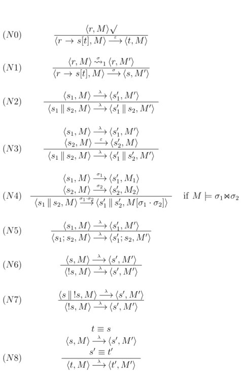
3.2 Semantics of the Coordination Language

The operational semantics of the coordination language is defined in Figure 3.3 as a labelled multi-step transition relation between configurations_hs, M_iwheresis a schedule and M is a multiset. The labels λ of transitions either denote a multiset substitution or the special symbol ε which indicates transitions that do not affect the multiset. The ε

symbol is a left and right unit for composition of multiset substitutions (·); i.e. ε·λ =

λ=λ·ε.

(34)

or more inference rules. The semantics of the schedule language is linked to that of the Gamma programs through the inference rules (N0) and (N1) for the rule condi-tional combinator. This construction enables the coordination language to schedule the individual computations as they are defined by the rules of a given Gamma program.

The set of semantic rules has been kept concise by identifying expressions that are structurally equivalent. A typical case is commutativity of parallel composition: “s1ks2”

and “s2ks1” are equivalent ways of writing down the same schedule. The ordering in

which the composition is written, should not make a difference. We therefore define a structural congruence “_≡” to be the smallest congruence relation over a set of terms such that a number of laws hold. Terms are thus grouped together on the basis of their syntax, allowing the semantic rules to focus on behavioural aspects of the terms. This method of separating structural from behavioural issues was inspired by work on the chemical abstract machine [15].

The structural congruences used by the operational semantics for schedules are given in Figure 3.2. Note that the use of the structural congruences (E6), (E7) and (E9) omit the need for explicit semantic rules for the conditional c ⊲ s[t] and recursion.

(E1) skip;s_≡s

(E2) s1; (s2;s3)≡(s1;s2);s3

(E3) skip_ks_≡s

(E4) s1ks2 ≡s2ks1

(E5) s1k(s2ks3)≡(s1ks2)ks3

(E6) true⊲ s[t]≡s

(E7) false ⊲ s[t]_≡t

(E8) !skip_≡skip

(E9) S(v)≡s[x:=v] if S(x)=b s

(35)

(N0) hr, Mi

√

hr → s[t], Mi ε

−→ ht, Mi

(N1) hr, Mi

σ

1hr, M′i

hr _→ s[t], M_i_{−→ h}σ s, M′_i

(N2) hs1, Mi

λ

−→ hs′1, M′i

hs1ks2, Mi

λ

−→ hs′

1ks2, M′i

(N3)

hs1, Mi

λ

−→ hs′₁, M′i hs2, Mi

ε

−→ hs′

2, Mi

hs1ks2, Mi

λ

−→ hs′

1ks′2, M′i

(N4)

hs1, Mi

σ₁

−→ hs′

1, M1i

hs2, Mi

σ₂

−→ hs′

2, M2i

hs1ks2, Mi

σ₁·σ₂

−→ hs′

1ks′2, M[σ1·σ2]i

if M _|=σ1⋊⋉σ2

(N5) hs1, Mi

λ

−→ hs′1, M′i

hs1;s2, Mi

λ

−→ hs′

1;s2, M′i

(N6) hs, Mi

λ

−→ hs′, M′i

h!s, M_i_{−→ h}λ s′_{, M}′_i

(N7) hsk!s, Mi

λ

−→ hs′, M′i

h!s, M_i_{−→ h}λ s′_{, M}′_i

(N8)

t_≡s

hs, M_i_{−→ h}λ s′_{, M}′_i

s′ _≡_t′

ht, Mi λ

−→ ht′, M′i

(36)

Analogous to the reflexive transitive transition relation for programs, we define the reflexive transitive closure of the transition relation for schedules.

Definition 3.2.1

hs, Mi−→h i *h_{s, M}i hs, Mi

λ

−→ hs′, M′i

hs, M_i_−→λ *hs′, M′i

hs, M_i λ1

−→*hs′, M′i

hs′_{, M}′_i λ₂

−→*hs′′, M′′i

hs, Miλ1·λ2

−→*h_s′′_{, M}′′i

The reflexive transitive transition relation uses labels λ which denote sequences of individual labels. For convenience we identify the singleton sequence _hλ_i with its only element λ. Furthermore, we use λb to denote the sequence λ where all occurrences of ε

have been removed.

Analogous to the case for Gamma programs, we define a capability function for schedules which models their input-output behaviour. The capability of a configuration is defined as the set of possible multisets it may produce, plus the special symbol ⊥ if the configuration may never terminate.

Definition 3.2.2 We define the “may diverge” predicate ↑ on configurations:

hs, M_i↑ if and only if

hs, M_i=_hs0, M0i and for all i≥0 there exists a λi such that hsi, Mii−→ hλi si+1, Mi+1i

Definition 3.2.3 The capability function _C : S×M → P(M)_{∪ {⊥}} for schedules, is defined as

C(s, M) = _{{⊥ | h}s, M_{i↑} ∪ {}M′ _{| h}_{s, M}_i λ

−→*h_skip, M′i}

3.2.1 Rationale for the Coordination Language

The behaviour of Gamma programs ranges from highly nondeterministic chaotic exe-cution to that of known algorithms. We want to be able to express all the possible behaviours of Gamma programs in the same formalism. To this end we designed the coordination language. The combinators that are present in the coordination language have been chosen for one of two reasons.

(37)

• For all practical purposes, we need the schedule-representation of any of these or-derings of actions to be finite. Some aspects of coordination strategies, like the number of iterations and the number of actions that can be executed in paral-lel, cannot in general be defined a priori. Hence we need constructs that evolve dynamically as a function of the input (rather than of the size of the input only). In order to define an ordering on actions we need to describe two things:

• the precedes/succeeds relations between actions. This is traditionally represented by the ‘;’ symbol: ‘s1;s2’ means that before the actions of ‘s2’ may be executed,

all actions of ‘s1’ must be finished.

• the fact that actions are unordered. In our setting of schedules, the unorderedness of actions means that they can be executed concurrently. We write ‘s1ks2’ to

indicate that independent actions of ‘s1’ and ‘s2’ may be executed concurrently.

Finite representations of potentially infinite schedules can only be obtained by oper-ators that evolve dynamically:

• Generally, the exact execution ordering of individual rules cannot be known in advance. Recursion is incorporated to describe iterations of arbitrary length. The unfolding of a recursive schedule typically depends on the given multiset. Choices based on the parameters of a schedule can be specified using the conditional con-struct ‘c ⊲ s[t]’.

• We do not know in advance how many rules may be executed concurrently at any stage in the computation. The schedule ‘!s’ may evolve dynamically into the number of copies of ‘s’ that is needed. Hence, replication describes an arbitrary degree of parallelism.

We briefly reflect on the differences between the way we use replication and the way it is used by Milner in his π-calculus [91].

(38)

In our setting, the replication of schedules (which correspond to Milner’s processes) is autonomous: the number of times a schedule is replicated can not be influenced by other schedules that are running in its context.

It is desirable that replication stops when the schedule/process that is spawned no longer contributes to the outcome of the computation. In theπ-calculus, the environment has control over the spawning of processes, hence the environment can decide when replication may stop. However, in our coordination language replication is autonomous, hence the ability to stop has to be built into the semantics of replication. This is achieved by the inclusion of the semantic rule (N6).

If we would use recursion to define this potentially finite behaviour, we would also need a combinator for (pre-emptive) nondeterministic choice. In Section 9.2.1 we describe this construction and explain why we do not want the combinator for nondeterministic choice in our kernel language.

3.2.2 Single-Step Transitions

The operational semantics of Figure 3.3 describes behavioural aspects of our coordination language. A particular aspect of interest is the parallelism in the behaviour of coordi-nation strategies. The transition system that we use to define the operational semantics of schedules is a multi-step transition system. Characteristic of multi-step transition systems is that multiple actions, in our case: multiset rewrites, may be captured by a single transition, thereby modelling the possibility of parallel execution. This contrasts tosingle-step transition systems, such as used in [66] to define the semantics of Gamma programs, where every individual transition corresponds to precisely one rewrite. An important feature of multi-step transition systems is that they distinguish parallel ex-ecution from interleaved exex-ecution which the single-step transition systems do not. In Section 9.2.3, we show that, due to this property, multi-step transition systems more adequately model parallel computation than single-step transition systems.

(39)

The one-to-one correspondence between transitions and rewrites, which holds for single-step transition systems, does not suffer from this combinatorial explosion, which makes it easier to reason about individual transitions.

To reduce the complexity of reasoning about multi-step transition, we next present a result which shows that every multi-step transition can be mimicked by a sequence of single-step transitions. This greatly facilitates reasoning about the behaviour of schedules because it can be used to reduce reasoning about parallel behaviour to reasoning about sequential behaviour.

The multi-step character of the semantics of the coordination language is due to in-ference rules (N3) and (N4). These inference rules cater for the derivation of transitions which model multiple concurrent rewrites. This observation allows single-step transitions to be characterized by their derivation tree.

Definition 3.2.4 If a transition _hs, M_i_{−→ h}λ s′_{, M}′_i_{is derived without using the}

seman-tics rules (N3) and (N4), it is called a single-step transition.

A property of the operational semantics in Figure 3.3 is that every multi-step tran-sition can be split into a sequence of single-step trantran-sitions which has the same effect on the multiset. This has as a consequence that sequential behaviour is a special case of parallel behaviour.

Lemma 3.2.5 If _hs, M_i_{−→ h}λ s′_{, M}′_i_{, then there exists a sequence of single-step}

transi-tions

ht0, M0i

λ₁

−→ ht1, M1i. . .−→λi . . .htn−1, Mn−1i−→ hλn tn, Mni

such that hs, Mi=ht0, M0i and htn, Mni=hs′, M′i and λ =λ1·. . .·λn.

Proof By transition induction: Assume that hs, Mi λ

−→ hs′, M′i is derived by some inference. We consider the the different ways in which the last step of this inference can be done.

• By (N0) or (N1). The transition is single-step by definition.

• By (N2), with s ≡ s1ks2, from hs1, Mi

λ

−→ hs′

1, M′i. Hence s′ ≡s′1ks2. Then by

the induction hypothesis there exists a sequence of single-step transitions

ht0, M0i

λ1

(40)

where _hs1, Mi=ht0, M0i,htn, Mni=hs′1, M′i and λ=λ1·. . .·λn.

By repeated use of (N2) we derive the following sequence of single-step transitions

ht0ks2, Mi

λ₁

−→ ht1ks2, M1i. . .−→λi . . .htn−1ks2, Mn−1i−→ hλn tnks2, M′i

• By (N3), with s_≡s1ks2, from hs1, Mi

λ

−→ hs′

1, M′i and hs2, Mi

ε

−→ hs′

2, Mi.

Hence s′ _≡ _s′

1ks′2. The induction hypothesis applies to both of these transitions.

This gives the following sequences of single-step transitions

ht1,0, M0i

λ₁

−→ ht1,1, M1i. . .−→λi . . .ht1,n1−1, Mn1−1i λn₁

−→ ht1,n1, Mn1i

where _hs1, Mi=ht1,0, M0i,ht1,n1, Mn1i=hs′1, M′iand λ =λ1·. . .·λn1;

ht2,0, Mi

ε

−→ ht2,1, Mi. . .

ε

−→. . ._ht2,n2−1, Mi ε

−→ ht2,n2, Mi

where s2 =t2,0, t2,n2 =s′2 and ε·. . .·ε=ε.

By repeated use of (N2) we derive the following sequences of single-step transitions

ht1,0kt2,0, Mi

ε

−→ ht1,0kt2,1, Mi

. . . _−→ε . . .

ht1,0kt2,n2−1, Mi ε

−→ ht1,0kt2,n2, Mi

and

ht1,0kt2,n2, Mi λ₁

−→ ht1,1kt2,n2, M1i . . . −→λi . . .

ht1,n1−1kt2,n2, Mn1−1i λn₁

−→ ht1,n1kt2,n2, M′i

The result follows by concatenating these sequences:

ht1,0kt2,0, Mi

ε

−→. . ._−→hε t1,0kt2,n2, Mi λ1

−→. . . λn1

−→ht1,n1kt2,n2, M′i

Clearly ε_·. . ._·ε_·λ1·. . .·λn1 =λ.

• By (N4), withs_≡s1ks2, fromhs1, Mi

σ1

−→ hs′

1, M1iandhs2, Mi

σ2

−→ hs′

2, M2iwhere

M |=σ1⋊⋉σ2 and σ =σ1 ·σ2. Hence s′ ≡s′1ks′2. From Lemma A.2.6 follows that

these transitions may be applied in arbitrary interleaved order; for instance

hs1, Mi

σ1

−→ hs′₁, M1i and hs2, M1i

σ2

(41)

Applying the induction hypothesis to each of these gives the following sequences of single-step transitions

hs1, Mi

λ₁

−→. . . λn1

−→hs′1, M1i and hs2, M1i

λ′₁

−→. . . λ

′

n₂

−→hs′2, M′i

where λ1·. . .·λn1 =σ1 and λ′1·. . .·λ′n2 =σ2. By repeated use of (N2) we derive

the following sequences of single-step transitions

hs1ks2, Mi

λ1

−→. . . λn1

−→hs′

1ks2, M1i and hs′1ks2, M1i

λ′₁

−→. . . λ

′

n2

−→hs′

1ks′2, M′i

We concatenate these sequences into

hs1ks2, Mi

λ₁

−→. . . λn1

−→hs′

1ks2, M1i

λ′₁

−→. . . λ

′

n₂

−→hs′

1ks′2, M′i

Andλ1·. . .·λn1 ·λ′1·. . .·λ′n2 =σ1·σ2 =σ.

• By (N5) with s_≡s1;s2. The proof is analogous to the case for (N2).

• By (N6), with s _≡!s, from _hs, M_i λ

−→ hs′_{, M}′_i_{. From the induction hypothesis}

follows that there exists a sequence

hs0, M0i

λ₁

−→ hs1, M1i. . .−→λi . . .hsn−1, Mn−1i

λn

−→ hsn, Mni

of single-step transitions such that _hs, M_i = _hs0, M0i, hsn, Mni = hs′, M′i and

λ1·. . .·λn =λ. For the first transition we use (N6) to derive h!s, Mi

λ₁

−→hs1, M1i

(which is single-step). Concatenation gives_h!s, M_i λ1

−→. . ._−→hλn s′_{, M}′_i_.

• By (N7), with s ≡!s, from hsk!s, Mi λ

−→ hs′, M′i. From the induction hypothesis follows that there exists a sequence

hs0, M0i

λ₁

−→ hs1, M1i. . .−→λi . . .hsn−1, Mn−1i−→ hλn sn, Mni

of single-step transitions where hsk!s, Mi = hs0, M0i, hsn, Mni = hs′, M′i and

λ1 ·. . .·λn = λ. For the first transition we use (N7) to infer h!s, Mi

λ₁

−→hs1, M1i

(which is single-step). Concatenation with the subsequent transitions gives

h!s, M_i λ1

−→. . ._−→hλn s′_{, M}′_i_.

• By (N8), from s ≡ t, s′ ≡ t′ and ht, Mi λ

(42)

there exists a sequence of single-step transitions

ht0, M0i

λ₁

−→ ht1, M1i. . .−→λi . . .htn−1, Mn−1i

λn

−→ htn, Mni

where_ht0, M0i=ht, Miand htn, Mni=ht′, M′iand λ1·. . .·λn=λ. From the first

and the last transitions of this sequence we infer, by (N8), _hs, M_i λ1

−→ ht1, M1i and

htn−1, Mn−1i−→ hλn s′, M′i(which are both single-step). Concatenation gives

hs, M_i λ1

−→ ht1, M1i. . .−→λi . . .htn−1, Mn−1i−→ hλn s′, M′i

3.3 Most General Schedules

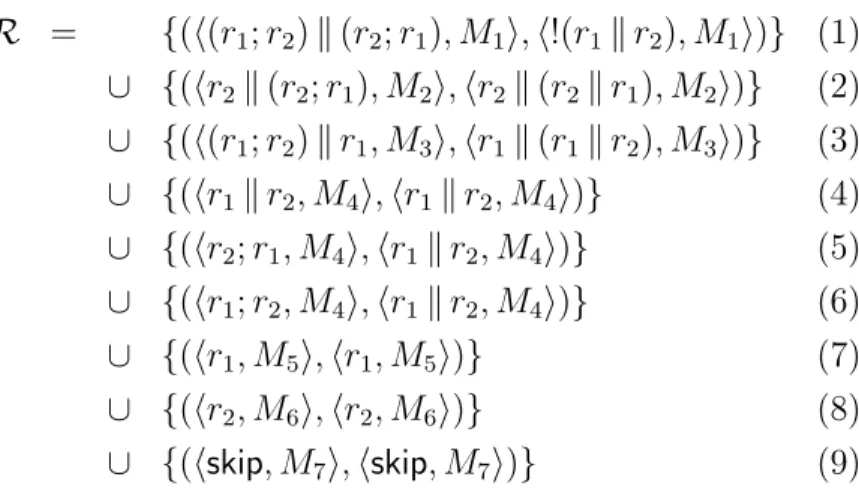
The coordination language allows us to specify behaviours from a wide spectrum of possibilities, ranging from the completely deterministic behaviour of known algorithms to the chaotic execution of Gamma programs. The latter can be seen by constructing a schedule that comprises all possible behaviours of a Gamma program. We refer to this schedule as the most general schedule . The most general schedule can be defined compositionally on the structure of Gamma programs (as given by the abstract syntax of Figure 2.2 in Chapter 2).

Definition 3.3.1 LetR denote a simple programr1+r2+· · ·rn and letP1 andP2 be two

arbitrary Gamma programs. The most general schedules for R and P1 ◦ P2 are defined

by

ΓR = ! (b r1 → ΓR k r2 → ΓR k · · · krn → ΓR)

ΓP1◦P2 = Γb P2; ΓP1

First, we give an informal explanation of the construction of the most general sched-ule. In the remainder of this chapter we formally prove the equivalence between Gamma programs and their most general schedule.

All rules ri of a simple programR are composed in parallel in ΓR such that initially

any (combination of) rule(s) may be executed. The replication that occurs in ΓR allows

(43)

the constituent rules may be executed in parallel. Successful execution of a rewrite rule may enable another rule, or re-enable itself. In order to avoid premature termination of the most general schedule, it is necessary that after the successful execution of a rule, every rule is tried (again) for execution. This is achieved by the recursive invocation of ΓR by every rule-conditional. The definition of ΓP1 ◦ P2 is straightforward.

Whereas the behaviour of Gamma programs is implicit in their representation, the most general schedule explicitly represents this behaviour. This explicit representation makes it amenable to formal manipulation. The particular kind of manipulation that we are interested in is refinement of behaviour. The fact that a most general schedule describes all possible behaviours of a corresponding Gamma program allows it to be used as the starting point in a process of refinement aimed at deriving more specific execution strategies. The techniques necessary for refinement will be developed in Chapter 4.

3.3.1 Completeness of the Most General Schedule

Most general schedules play an important rˆole in the process of refinement. They provide the initial description of the behaviour of Gamma programs. The central theme of this section is to show that the most general schedule deserves its name. To this end, we show that the most general schedule satisfies the following properties:

• Firstly, the most general schedule describes all possible ways of executing a Gamma program, but no more.

• Secondly, the input-output relation of a most general schedule matches that of the corresponding Gamma program.

In order to prove the above properties, we will introduce some auxiliary results and notation related to most general schedules.

Definition 3.3.2 Let P =r1+· · ·+rn and let ΓP be its most general schedule.

ΠP ≡ (r1 → ΓPk · · · krn → ΓP)

∆P,i ≡ (r1 → ΓPk · · · kri−1 → ΓPkri+1 → ΓP k · · · krn → ΓP)

A term ∆P,idiffers from ΠP because it misses theithtermri → ΓP. From commutativity

and associativity of parallel composition (k) follows that ΠP ≡(ri → ΓP)k∆P,i. Note

(44)

We introduce the notion of derivedness. This notion relates a configuration to the configurations that it may evolve into by execution.

Definition 3.3.3

1. We say that a configuration _hs′_{, M}′_i _is _h_{s, M}_i_{-derived if} _h_{s, M}_i λ

−→*hs′, M′i for

some λ. This is also denoted _hs, M_{i −→}*hs′, M′i.

2. We say that a schedule s′ is s-derived if hs, Mi −→*hs′, M′i for some M and M′. The predicate µis used to denote a class of schedules which satisfy a certain syntac-tical format whose importance will be illustrated shortly by Lemma 3.3.7.

Definition 3.3.4 Let S= !(b r1 → Sk . . . krn → S).

1. We write µS(s) if s ≡ (r1 → S)a1k . . .k(rn → S)ankSk with ai ≥ 0 for all i :

1≤i≤n and k ≥0.

2. We write µ+_S(s) if µS(s) with k ≥1; in other words s ≡s′kS where µS(s′).

Next, we extend the use of predicate µto configurations.

Definition 3.3.5 LetS= !(b r1 → Sk . . .krn → S). We writeµS(s, M), if the following

conditions hold for _hs, M_i:

1. s≡(r1 → S)a1k . . .k(rn → S)ankSk with ai ≥0 for all i: 1≤i≤n and k ≥0

2. (k= 0) _⇒ (_∀i: 1_≤i_≤n :ai = 0 ⇒ [[†ri]]M)

Next, we show thatµΓP describes a relation between schedule and multiset that holds

for any_hΓP, Mi-derived configuration (for some simple programP). To this end, we first

observe that the configuration_hΓP, MisatisfiesµΓP (for anyM and simpleP). Secondly

we prove that property µS (for configurations) is invariant with respect to sequences of

multi-step transitions.

The proof of invariance of µS with respect to sequences of multi-step transitions

is structured as follows: First we show invariance of µS with respect to single-step

(45)

Lemma 3.3.6 If µS(s, M) and hs, Mi

λ

−→ hs′_{, M}′_i _{is a single-step transition, then}

µS(s′, M′).

Proof From µS(s, M) follows s ≡ (r1 → S)a1k . . . k(rn → S)ankSk with ai ≥ 0 for

alli: 1≤i≤n and k ≥0 such that (k = 0) ⇒ (∀i: 1≤i≤n:ai = 0 ⇒ [[†ri]]M).

We show µS(s′, M′) by induction onk.

• k = 0: By transition induction can be shown that a single-step transition can be derived in one of the following ways.

– By (N0) fromhri, Mi√ for some i. Hence λ=ε and M′ =M. Thena′j =aj

for all j 6=i,a′i =ai −1 and k′ =k. HenceµS(s′, M′).

– By (N1) from hri → S, Mi

σ

−→ hS, M′_i_{, for some} _i_{. Hence} _λ ₌ _σ_{. Then}

a′_j =aj for all j 6=i,a′i =ai−1 andk′ =k+ 1. Hence µS(s′, M′).

• k > 0: By transition induction can be shown that a single step transition can be derived in one of the following ways.

– By (N0) or (N1). The proof proceeds analogously to the casek = 0.

– By (N8) from unfolding the definition of S. A transition can be derived from_hs′′_{, M}_i λ

−→ hs′_{, M}′_i_where_s′′ _≡₍_r

1 → S)a

′′

1 k . . .k(r_n → S)a′′nkSk′′with a′′

j =aj+ 1 for allj and k′′=k−1. ThenµS(s′′, M), hence the result follows

by the induction hypothesis.

Now, we use the invariance of µS over single-step transitions to prove the invariance

over multi-step transitions.

Lemma 3.3.7 If µS(s, M) and hs, Mi

λ

−→ hs′_{, M}′_i_{, then} _µ

S(s′, M′).

Proof By Lemma 3.2.5 follows that there exist λ1, . . . , λn, n≥1 such that

hs0, M0i

λ1

−→ hs1, M1i. . .−→λi . . .hsn−1, Mn−1i−→ hλn sn, Mni

where hs, Mi = hs0, M0i and hsn, Mni = hs′, M′i and each transition

Separating computation and coordination in the design of parallel and distributed programs

in the Design of Parallel and Distributed

Programs

Contents

1

Introduction

Structure of this thesis

2

The Computational Model

2.1

The Gamma Programming Model

2.2

Reasoning about Gamma Programs

2.3

Concluding Remarks

3

The Coordination Model

3.1

The Coordination Language

3.2

Semantics of the Coordination Language

3.2.1

Rationale for the Coordination Language

3.2.2

Single-Step Transitions

3.3

Most General Schedules

3.3.1

Completeness of the Most General Schedule