Sharif University of Technology
Scientia IranicaTransactions E: Industrial Engineering http://scientiairanica.sharif.edu
A novel fuzzy multi-objective method for supplier
selection and order allocation problem using NSGA II
M.A. Sobhanolahi, A. Mahmoodzadeh
, and B. Naderi
Department of Industrial Engineering, Faculty of Engineering, Kharazmi University, Tehran, Iran. Received 21 February 2018; received in revised form 27 July 2018; accepted 15 October 2018
KEYWORDS Supplier selection; Order allocation; Fuzzy theory; Multi-objective programing; NSGA II.
Abstract. This paper introduces a supplier selection and order allocation problem in a single-buyer-multi-supplier supply chain in which appropriate suppliers are selected and orders allocated to them. Transportation costs, quantity discount, fuzzy-type uncertainty, and some practical constraints were taken into account in the problem. The problem was formulated as a bi-objective model to minimize annual supply chain costs and to maximize Annual Purchasing Value (APV). The fuzzy weights of suppliers, which were the output of one of the supplier evaluation methods, were considered in the second objective function. Then, a novel fuzzy multi-objective programming method was formulated for obtaining Pareto solutions. The method is the extension of a single-objective method existing in the literature. It is based on the degree of satisfaction of the Decision Maker (DM) with each fuzzy objective considering the fulllment level of fuzzy constraints. In the proposed method, the problem remains multi-objective and, unlike in the existing methods, it is not transformed into a single-objective model. At the last stage of the proposed method, the fuzzy results are compared with an index and the DM can identify the appropriate or inappropriate solutions. To solve the problem, Non-dominated Sorting Genetic Algorithm (NSGA II) is designed and computational results are presented using numerical examples. © 2020 Sharif University of Technology. All rights reserved.
1. Introduction
In the current competitive environment, supplier eval-uation and selection is one of the most important processes in supply chain management for any orga-nization. It is critical since suppliers have a major impact on strategic and operational performance of organizations. Also, this process plays an important role in determining the cost, quality, and other aspects of the nished product [1]. Hence, organizations rely
*. Corresponding author. Tel.: +98 26 34551022 E-mail addresses: [email protected] (M.A. Sobhanolahi); [email protected] (A. Mahmoodzadeh); [email protected] (B. Naderi) doi: 10.24200/sci.2018.50484.1717
more on suppliers to reduce their costs, to improve the quality of their products, or to focus on a specic part of their operations [2].
Supplier selection is complex since organizations must take into account multiple aspects including both quantitative and qualitative criteria [3,4]. In such cases, the criteria are conicting and a trade-o among them is required. Therefore, selection of the best suppliers becomes a multi-criteria decision-making problem. Furthermore, the process becomes more complicated if parameters are incomplete or uncertain. On the other hand, higher levels of inventory lead to increased supply chain responsiveness, but decrease cost eciency because of inventory holding costs [5]. Inventory costs account for a number between 20 and 40% of the total product value. Hence, inventory management is one of the signicant parts
of supply chain management [6]. Allocating orders to the selected suppliers allows for some economies of scale through the right choice of quantities to order from each supplier. Sometimes, suppliers oer quantity discounts as a powerful incentive to motivate buyers to increase the amount of their ordered quantities [7]. Indeed, the unit price paid by buyers for large orders is usually smaller than the unit price of small orders [8]. Incremental quantity discounts, business volume quantity discounts, and all-unit quantity discounts are the three main types of quantity discounts [9].
This paper introduces a supplier selection and or-der allocation problem in a single-buyer-multi-supplier supply chain in which appropriate suppliers are selected and orders allocated to them. Transportation costs, quantity discount, fuzzy-type uncertainty, and some practical constraints are taken into account in the problem. Firstly, the problem is formulated as a bi-objective model for minimizing annual supply chain costs and maximizing Annual Purchasing Value (APV). The fuzzy weights of suppliers, which are the output of one of the supplier evaluation methods, are considered in the second objective function. The assumptions of the model are appropriate to the real-world conditions. Therefore, the model can be applied to any type of supply chain in which a buyer acquires the demanded items from some potential suppliers.
To overcome the complexity of the process, we propose a novel fuzzy multi-objective programming method for obtaining Pareto solutions. The method is an extension of the single-objective method proposed by Jimenez et al. [10]. It is based on the level of satisfaction of the Decision Maker (DM) with each fuzzy objective considering the degree of realization of fuzzy constraints. In the proposed method, the prob-lem remains multi-objective and, unlike in the existing methods, it is not transformed into a single-objective model. At the last stage of the proposed method, the fuzzy results are compared with an index and the DM can identify the appropriate or inappropriate solutions. To solve the problem, Non-dominated Sorting Genetic Algorithm (NSGA II) is designed and computational results are presented using numerical examples.
The rest of this paper proceeds as follows. In Section 2, the related literature is briey reviewed. In Section 3, we describe the problem, state the assumptions, and give the parameters, variables, and the formulation of the model. Section 4 deals with the novel fuzzy multi-objective programming method. Section 5 is devoted to describing the solution proce-dure, including changes in objectives and constraints, solution encoding, repair algorithm, and NSGA II procedure. In Section 6, we illustrate the ndings of the implementation of the proposed methodology with some numerical examples. Finally, Section 7 concludes the study and presents future research directions.
2. Literature review
2.1. Supplier selection and order allocation In this section, the researches which have been con-ducted in the area of supplier selection and order allocation with quantity discount are reviewed and their objectives and solution methods are addressed. Dahel [11] assumed multi-item volume discounts and proposed a multi-objective mixed-integer program-ming model, which could be solved through either a preference-oriented approach or the generating ap-proach. Demirtas and Ustun [12] studied a model to maximize the purchasing value and to minimize the budget and the defect rates. They used analytical network process and the multi-objective mixed-integer programming, and adopted epsilon-constraint method and reservation level through Tchebyche procedure to solve the problem. Xia and Wu [13] studied a problem to maximize total weighted quantity of purchasing, minimize total purchasing cost, minimize the number of defective items, and maximize the number of on-time delivered items. They proposed a two-stage method to solve the problem by means of Analytical Hierarchy Process (AHP) improved by rough set theory, at the rst stage, and a multi-objective mixed-integer linear programming, at the second stage. Burke et al. [14] considered three types of discounts, namely linear quantity discount, incremental unit price discount, and all-unit quantity discount. They developed a heuristic to measure the eect of quantity discounts in the problem. Kokangul and Susuz [15] investigated a bi-objective model by minimizing total purchasing cost and maximizing purchasing value obtained using AHP. They proposed a bi-objective non-linear programing model using goal programming. Amid et al. [16] stud-ied a model which minimized total cost, the percentage of late-delivery items, and the percentage of rejected items. They developed a fuzzy multi-objective mixed-integer linear programming model to solve the problem. Wang and Yang [17] developed a model to minimize total cost, defective rate, and delivery lateness rate and proposed a two-stage procedure using AHP and a multi-objective mathematical programming. Ebrahim et al. [18] developed a model to minimize cost, late delivered items, and defective items considering three types of discount and proposed a Scatter Search (SS) algorithm and exact method to solve the problem. Razmi and Maghool [19] considered three types of discount in a fuzzy bi-objective model to minimize total purchasing cost and maximize total purchasing value. They adopted an augmented epsilon-constraint and reservation level by Tchebyche models. Kamali et al. [20] investigated a model to minimize total annual cost, total number of defective items, and total number of late delivered items as well as to maximize total purchasing value. They proposed Particle Swarm
Op-timization (PSO) and SS algorithm to solve the model. Zhang and Zhang [21] studied a single-objective model to minimize costs with stochastic demand and solved a mixed-integer programming in which all suppliers met the qualitative criteria level. Lee et al. [22] investigated a single-objective model to minimize total purchasing cost under all-unit and incremental quantity discounts and designed a genetic algorithm to solve the model. Pazhani et al. [5] addressed a single-objective model to minimize total cost per unit time considering the purchasing, setup, holding, and transportation costs. A mixed-integer nonlinear programming model was developed to solve the problem using exact methods. Moghaddam [23] set the four objectives of maximizing total net prot and minimizing total defective parts, total late deliveries, and total risk factors of the economic environment associated with each supplier. Bohner and Minner [24] considered both all-units and incremental quantity discounts as well as failure risk to minimize total costs and solved the mixed-integer linear programming model using an exact approach. Cebi and Otay [25] developed a model to minimize total cost, total late deliveries, and total defective items and to maximize total utility of the purchasing activity. Hamdan & Cheaitou [1] considered green criteria to maximize total value of purchasing and minimize total costs. They proposed a three-stage method using fuzzy TOPSIS at the rst stage to assign two preference weights to every potential supplier, AHP at the second stage to determine the importance weight of each sup-plier, and bi-objective integer linear programming at the third stage. The model was solved by the weighted comprehensive criterion method and the branch-and-cut algorithm. Hamdan and Cheaitou [26] dealt with green criteria, quantity discounts, and varying supplier availability and applied the same three-stage method proposed in their previous study [1] in order to max-imize total green and traditional values of purchasing and minimize total purchasing cost. Ranjbar Tezenji et al. [27] considered supplier location selection and order allocation under capacity constraints in a stochastic environment. The objective function included estab-lishment, inventory, and transportation costs. They developed a bi-objective model for optimization of the mean and variance of costs and solved the model by genetic algorithm and simulated annealing.
In this paper, we assume two common objectives of minimizing total costs and maximizing purchasing value.
2.2. Fuzzy multi-objective approaches
There are some methods in the literature for ag-gregating fuzzy goals and constraints. Jimenez and Bilbao [28] proposed a method for multi-objective pro-gramming problem with fuzzy objectives to maximize P
ifi(x) subject to Zf(x) , with representing
the degree of satisfaction of DM with the achievement of goals. A unique optimal solution to the above problem is the ecient fuzzy solution to the original Multi Objective Problems (MOPs) [29]. There are some approaches such as the weighted additive ap-proach [30,31], compromise apap-proach [32], the method with achievement degrees [33], augmented max-min model [34,35], and two-phase approach [36] in the literature, which ensure the existence of an ecient fuzzy solution. Moghaddam [23] applied fuzzy goal programming approach to the supplier selection and order allocation problem in reverse logistics systems. He utilized a Monte Carlo simulation integrated with fuzzy goal programming to determine the entire set of Pareto optimal solutions. By incorporating the linear membership functions for objectives and constraints in other constraints, he formulated a fuzzy goal pro-gramming model. Erginel and Gecer [37] investigated a fuzzy multi-objective linear programming model for the supplier selection problem. Weight, cost, and calibration time were handled as fuzzy numbers for modelling the imprecise data. A two-phase approach was used to obtain a Pareto optimal solution and solve the fuzzy multi-objective decision model. Cebi and Otay [25] studied the supplier selection and order allocation problem considering quantity discounts and lead time. They applied a two-stage fuzzy approach to solving the problem and used the augmented max-min model, guaranteeing non-domax-minated solutions, to transform the fuzzy multi-objective model into a crisp single-objective one. To select suppliers, they utilized fuzzy MULTIMOORA at the rst stage and fuzzy goal programming, to determine order amounts at the second stage. Govindan et al. [38] addressed the sup-plier selection problem with transportation decisions in an eco-ecient closed-loop supply chain network by utilizing weighted fuzzy mathematical programming approach to generating a properly ecient fuzzy solu-tion. They rst dened linear membership functions for each fuzzy goal as introduced by Zadeh [39] and then, applied a weighted max-min approach to searching for an optimal solution. Their aim was to make the levels of achievement of the goals and the weights of the goals as close to each other as possible.
As observed in the review of the literature, all fuzzy approaches transform a model into a single-objective one. However, in this paper, we propose a method to solve a problem in its original multi-objective form.
3. Problem formulation
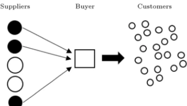
Assume that a supply chain includes a buyer and several suppliers. The buyer intends to evaluate suppliers and allocate orders to them, as shown in Figure 1. Thus, the buyer faces a supplier selection and
Figure 1. Schematic view of supply chain.
order allocation problem. The main objectives of the buyer are to minimize annual supply chain costs and maximize APV so that they do not face any shortages. The main assumptions of the problem are as follows:
There is only one single product involved; the buyer can purchase their required amount from several suppliers;
The annual demand is known and constant over time;
Each supplier has a specic production capacity;
Inventory shortage is not allowed for any supplier or buyer;
The inventory cannot be transferred from period to period;
The transportation cost from each supplier to the buyer depends on the distance and the number of required vehicles;
The defective rate of each supplier is known;
In each period, the (i + 1)th order by the supplier cannot be entered unless the whole ith order is consumed;
All suppliers use the price discount policy to en-courage the buyer to place large orders. Suppose that there are n suppliers in the supply chain. Each supplier i uses the quantity discount policy, which includes Ki price levels, and the kth price level is
determined by price cikand order range [ui;k 1; uik).
The logical assumption is that for ui1< ui2< ::: <
ui;Ki, we have ci1> ci2> ::: > ci;Ki.
The model studied in this research has some similarities with those of Kamali et al. [20] and Alaei and Khoshalhan [40]. They also considered the problem as a multi-objective programming model for maximizing APV and minimizing annual supply chain costs, defective items, and late deliveries. To solve the model, Kamali et al. [20] utilized PSO and SS; in addition to PSO and SS, Alaei and Khoshalhan [40] used the harmony search and the hybrid harmony-cultural algorithm. However, while the above papers
both dealt with the problem in deterministic environ-ment, in this study, the problem is considered as a bi-objective optimization model with fuzzy parameters for objectives and constraints. Therefore, a novel method is proposed for obtaining Pareto solutions to the fuzzy bi-objective problem. The method is an extension of the single-objective method proposed by Jimenez et al. [10]. We also utilize NSGA II to solve the problem. 3.1. Notation
The following parameters and decision variables are to be used in the model.
Parameters
D Annual demand rate of the buyer Si Fixed production setup cost to supplier
i
Ai Fixed ordering cost for supplier i
hi Inventory holding cost to supplier i per
unit per unit time
hb Inventory holding cost to buyer per
unit per unit time
Ti Consumption time of an order quantity
from supplier i
T Length of period for the buyer ci Variable cost per unit (fuzzy) to
supplier i
cik Discounted unit price of interval k
oered by supplier i
Pi Production rate of supplier i
uik Upper bound of discount interval for
supplier i
ri Defective rate (fuzzy) for supplier i
R Maximum acceptable defective rate for all purchased quantities
disi Distance between buyer and supplier i
cap Capacity of vehicles
C Fixed cost of transportation per distance unit (fuzzy)
Wi Importance rate of supplier i in
supplier evaluation methods (fuzzy) Decision variables
qik Purchased quantity per period from
supplier i in discount interval k yik Binary variable equal to 1 if qik falls
into discount interval k of supplier i, 0 otherwise
Qi Order quantity from supplier i per
period
Q Total order quantity per period from all suppliers
Zi Integer variable denoting the number
3.2. Model
The mathematical modeling of the problem is shown as a mixed-integer nonlinear programming model as follows:
Min Cost =DQ Xn
i=1 Ki
X
k=1
(~ci+ cik) qik
+
n
X
i=1 Ki
X
k=1
(Ai+ Si) yik
+
n
X
i=1
Q2 i
2
hb
D+ hi
Pi
+
n
X
i=1
~ CdisiZi
;
(1)
Max AP V = DQXn
i=1
~
wiQi; (2)
Qi= Ki
X
k=1
qik 8i = 1; :::; n; (3)
Q =
n
X
i=1
Qi; (4)
D
QQi Pi 8i = 1; :::; n; (5) cap (Zi 1) Qi 8i = 1; :::; n; (6)
Qi capZi 8i = 1; :::; n; (7) Ki
X
k=1
yik 1 8i = 1; :::; n; (8)
ui;k 1yik qik 8i = 1; :::n; 8k = 1; :::; Ki; (9)
qik uikyik 8i = 1; :::; n; 8k = 1; :::; Ki; (10)
1 Q
n
X
i=1
Qi~ri R; (11)
yik2 f0; 1g 8k = 1 : Ki; i = 1; :::; n; (12)
Zi2 Integer 8i = 1; :::; n; (13)
qik 0 8k = 1 : Ki; i = 1; :::; n; (14)
Qi 0 8i = 1; :::; n; (15)
Q 0: (16)
Eq. (1) minimizes the cost objective function, which consists of four parts. The rst part involves variable and purchase costs; the second part includes order-ing and setup costs; the third part is the inventory holding costs to the buyer and to suppliers; and
the fourth part calculates the transportation costs. Eq. (2) maximizes the total APV, which determines the weighted quantities of orders. These weights specify the importance of suppliers and can be the output of the multi-criteria decision-making methods [25]. This maximization relation leads to allocating more orders to more important suppliers. Eq. (3) states that the sum of purchases in the discount intervals of a supplier is equal to the amount of purchases from that supplier. Based on Eq. (4), the total purchase of the buyer in each cycle is equal to the sum of purchases from all suppliers. Capacity constraints of the suppliers are expressed by Eq. (5). The number of required vehicles to carry the products of each supplier is calculated using Eqs. (6) and (7). Eq. (8) ensures that the order to each supplier is only at one of its discount intervals. Through Eqs. (9) and (10), the order to each supplier falls into one of the discount intervals oered by the supplier. Eq. (11) ensures that the rate of defective products does not exceed a predetermined value. Finally, Relations (12){(16) dene the types of variables.
4. Fuzzy multi-objective approach
Various methods have been presented in the literature for fuzzy multi-objective optimization. However, we propose a novel method for the problem, which is based on satisfaction degree of the DM with fuzzy objectives and the level of fullment of the constraints. This method is an extension of the single-objective fuzzy programming proposed by Jimenez et al. [10] to the multi-objective environment. The method aims to identify the Pareto solutions which best match the desires of the DM. Fuzzy objective functions are replaced by the degree of satisfaction dened in the algorithm and fuzzy constraints are rewritten as a function of , which represents the level of fullment.
Step 1. According to Jimenez et al. [10], fuzzy constraints must be rewritten as a function of alpha. With these modications, the problem space becomes wider for = 0 and more limited for = 1. For any constraint type \," fuzzy coecient ~a = (a1; a2; a3)
and fuzzy right-hand side ~b = (b1; b2; b3) should be
replaced by the following expressions, respectively:
~a (1 )
a1+ a2
2
+
a2+ a3
2
; (17)
~b b1+ b2
2
+ (1 )
b2+ b3
2
: (18)
Step 2. The DM is asked to specify the interval G; Gfor each objective. For a minimization objec-tive, if z G, they will nd it totally satisfactory; but if z G, their degree of satisfaction will be null.
Accordingly, the goal is expressed by means of a fuzzy set ~G whose membership function is as follows:
G~(z) =
8 > < > :
1 if z G
[0; 1] decreasing on G z G 0 if z G (19) Similarly, we dene ~G for maximization objectives as follows.
G~(z) =
8 > < > :
1 if z G
[0; 1] increasing on G z G 0 if z G (20) The DM aims to gain the maximum degree of satis-faction. However, in order to get a better objective value, a lower level of fullment of constraints is considered. Given these circumstances, the DM might want a lower satisfaction degree of objectives in exchange for a better level of fullment of con-straints [10].
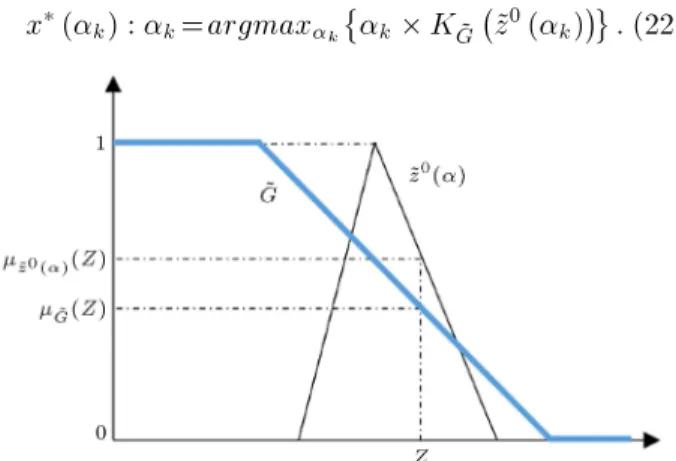
Step 3. For each objective, we need to compute the satisfaction degree of the fuzzy goal ~G by each -acceptable Pareto solution, that is, the membership degree of each fuzzy number ~z0(k) in the fuzzy
set ~G. There are several methods for this purpose (e.g., [41]. We will apply the index proposed by Yager [42] and used by Jimenez et al. [10] as follows:
KG~ z0()= s +1
1~z0()(z) G~(z) dz
s+11~z0()(z) dz ; (21)
where the denominator is the area under ~z0()
and, in the numerator, the possibility of occurrence ~z0()(z) for each crisp value z is weighted by its
satisfaction degree G~(z) for goal ~G (see Figure 2).
Step 4. Here, in order to achieve a balance between satisfaction degree and constraints fullment level, we use the condition similar to that considered by Jimenez et al. [10] as follows:
x(
k) : k=argmaxk
k KG~ ~z0(k) : (22)
Figure 2. Occurrence possibility of a crisp objective value, z, and its goal satisfaction degree.
The greater the value of , the more limited the problem space and the lower the satisfaction degree and vice versa. By using the above equation, a trade-o between and satisfactitrade-on degree can be achieved. Step 5. The solutions for each fuzzy objective func-tion can be compared and the DM can identify the appropriate or inappropriate solutions among Pareto solutions through the following two denitions: Denition 1: For any pair of fuzzy numbers ~a and ~b, the degree in which ~a is greater than ~b is calculated as follows [10]:
M
~a; ~b= 8 > > < > > :
0 if Ea
2 Eb1< 0 Ea
2 E1b
(Ea
2 Ea1)+(E2b Eb1) if
Ea
1 E2b; E2a E1b
< 0 1 if Ea
1 Eb2> 0 (23)
where [Ea
1; E2a] and
Eb
1; Eb2
are the expected inter-vals of ~a and ~b. We say that ~a and ~b are indierent if M
~a; ~b= 0:5.
Denition 2: For a triangular fuzzy number ~a = (a1; a2; a3), the expected interval is easily calculated
as follows [43]: EI (~a) = [Ea
1; E2a] =
a1+ a2
2 ;
a2+ a3
2
: (24) 4.1. The case of trapezoidal fuzzy numbers The proposed method can also be applied to trape-zoidal fuzzy numbers. In Step 1, for any fuzzy coecient ~a = (a1; a2; a3; a4) and fuzzy right-hand
side ~b = (b1; b2; b3; b4), Relations (17) and (18) can be
rewritten as [10]: ~a (1 )
a1+ a2
2
+
a3+ a4
2
; (25)
~b b1+ b2
2
+ (1 )
b3+ b4
2
: (26) In Denition 2 of Step 5, for a fuzzy number ~a = (a1; a2; a3; a4), the expected interval will be [43]:
EI (~a) = [Ea 1; E2a] =
a1+ a2
2 ;
a3+ a4
2
: (27) The other steps remain unchanged.
5. Solution procedure
The dened problem in the previous section is nonlin-ear. The reason is that the variable Q is the denomina-tor of Eqs. (1), (2), (5), and (11). Certainly, Eq. (5) can be converted to a linear form, DQi PiQ. The linear
form of Eq. (11) can also be rewritten asPn
However, Relations (1) and (2) are totally nonlinear. Considering that nonlinear problems cannot be solved by exact methods, NSGA II is designed for solving the problem in hand. Firstly, the fuzzy objective functions and the fuzzy constraints must be modied in accordance with the proposed method.
5.1. Modication of fuzzy objectives and fuzzy constraints
Given the rst step of the proposed method, assuming that eri = ri1; r2i; ri3
, Eq. (11) can be rewritten as follows: n X i=1 Qi (1 ) r1
i + ri2
2
+
r2 i + ri3
2
QR: (28) It is also assumed that the fuzzy values of the objec-tive functions in a solution are denoted by ]Cost = (1; 2; 3) and ^AP V = (1; 2; 3). The interval G; G
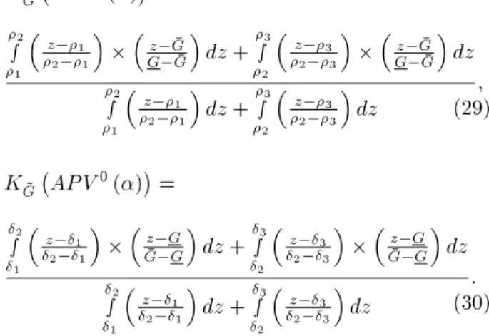
of each objective can be determined by the DM. Here, we assume that the ideal value of each objective is determined by optimizing the function and ignoring the other one. Also, the non-ideal value is determined by the DM. In optimizing each objective, the problem is solved for the smallest possible amount of , which ensures that the problem space is in the broadest state. Then, the degree of satisfaction of objectives can be calculated as follows:
KG~ Cost0()= 2
s
1
z 1
2 1
z G G G
dz +s3
2
z 3
2 3
z G G G
dz 2 s 1
z 1
2 1
dz +s3
2
z 3
2 3
dz (29);
KG~ AP V0()
= 2 s 1
z 1
2 1
G Gz G
dz +s3
2
z 3
2 3
G Gz G
dz 2 s 1
z 1
2 1
dz +s3
2
z 3
2 3
dz
: (30)
It should be noted that the objective functions in Eqs. (1) and (2) are minimization and maximization, respectively. Thus, the membership function of ~G is descending for the rst objective and ascending for the second one. The integrals of the above relations can be easily calculated.
5.2. Solution representation
Each chromosome or answer vector can be expressed as Q : [Q1; Q2; : : : ; Qn]; the sum of the vector is equal
to Q. Qi represents the order quantity assigned to
supplier i and it is equal to Qi : [qi1; qi2; : : : ; qi;Ki].
The procedure for generating initial solutions is shown in Figure 3.
Figure 3. Procedure of the initial solution generation.
5.3. Repair algorithm
Due to the existence of constraints in the problem, it is possible to face infeasible solutions in the initial solution generation algorithm and repetition of the main algorithm. These infeasible solutions must be controlled using the constraints handling methods. In this section, we propose a repair algorithm, which transforms infeasible solutions to feasible ones. Eqs. (3) and (4) are established by solution representation. By calculating the number of vehicles, Eqs. (6) and (7) are enforced. Eqs. (8){(10) are also established according to the order quantity from each supplier, which should fall into one of the discount intervals. The only constraints that may lead to infeasible solutions are Eqs. (5) and (25). In the following, we propose a repair algorithm for them:
- Repair Algorithm 1: In an infeasible solution, according to Eq. (5), for each supplier i, we dene ai = Pi DQi=Q. If ai > 0, then the supplier
still has some capacity for order assignment. On the other hand, if ai < 0, the amount of annual
order assigned to the supplier exceeds its annual production capacity. Therefore, we dene two sets of S+ = fi : a
i 0g and S = fi : ai 0g. The
set S+ represents the suppliers with an additional
capacity for assignment and the set S represents the suppliers whose capacity constraints are violated. The following changes ensure the feasibility of a solution if we havePi2S+aiPi2S ai; otherwise,
the solution is rejected:
Qi= QDPi 8i 2 S ; (31)
Qi= Qi+
ai
P
i2S+ai
X
i2S
ai 8i 2 S+: (32)
According to Eq. (31), the annual order quan-tity from suppliers with violated capacity constraint is set equal to their annual production rate. Eq. (32) shares the additional order quantity (Pi2S ai)
among other unviolated suppliers in proportion to their available capacities.
- Repair Algorithm 2: For Eq. (28), we dene: A =X
i=1Qiri0 QR
ri0 =(1 ) r1i + ri2+ r2i + r3i=2:
Also, due to changes in Repair Algorithm 1, ai is
re-calculated for all suppliers and the sets S+ and
S are formed. If we have A > 0, the constraint is violated. Thus, two suppliers i and j are randomly chosen, provided that we have r0
i > r0j and j 2 S+.
Then, modications Qj = Qj+ 0 and Qi = Qi
0 must be applied. In this case, it is guaranteed
that the total order quantity (Q) is not changed. Reducing the order quantity from supplier i does not lead to any violation. However, increasing it may lead to exceeding the production capacity constraint. Therefore, consider the following changes:
= r0 A
i r0j; (33)
0 = min f; a
j; Qig : (34)
Eq. (33) determines the amount which must be reduced from the order quantity from supplier i and added to the order quantity from supplier j. This change should be considered in accordance with Repair Algorithm 1. Therefore, according to Eq. (34), the minimum dierence between the amount determined in Eq. (33) and the remaining capacity of supplier j, aj, must be selected. Also,
to prevent negative values for Qi, the minimum
dierence between Qi and the determined value
should be chosen. It should be noted that the procedure is repeated until the value of A is positive. If repair is not performed within the predened replications, the solution modications of Repair Algo-rithm 2 are ignored and Repair AlgoAlgo-rithms 1 and 2 are repeated again.
5.4. Non-dominated Sorting Genetic Algorithm (NSGA II)
NSGA II was presented by Deb et al. [44] as one of the best algorithms for obtaining Pareto frontiers. In this algorithm, the population P1 is generated with
respect to population size Np. At repetition t, after
selecting parent chromosomes from population Pt, the
ospring (population Ot) are generated according to
the crossover rate pc and the mutation rate pm. Then,
Pt is merged with Ot and chromosomes are sorted
into non-dominated frontiers based on their rank and crowding distance. Np best solutions form population
Pt+1. The algorithm continues until the best Pareto
solutions are obtained in accordance with the stop condition. For more information, see Deb et al. [44] and Deb [45].
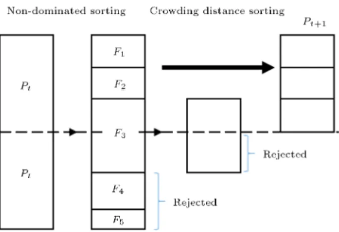
A graphical view of the algorithm is shown in Figure 4. After non-dominated sorting, the solutions are sorted into Fi frontiers, where F1 is the best
Pareto frontier. The chromosomes within each frontier are also sorted according to the crowding distance.
Figure 4. Graphical view of NSGA II.
After merging parents and ospring populations, the best frontiers are transferred to the new population. As shown in Figure 4, the frontiers F1 and F2 and
the chromosomes with higher crowding distances on frontier F3 are transferred to the new population and
the other frontiers are eliminated.
In the proposed algorithm, we utilize a uniform crossover. Assume that chromosomes m and n are selected. After choosing a random number in the interval (0; 1), the order quantities for each supplier i in ospring 1 and 2 are determined by Q1
i = Qmi +
(1 ) Qn
i and Q2i = (1 ) Qmi + Qni, respectively.
In addition, if a mutation is applied to the chromosome, one supplier is randomly selected and its order quantity is exactly determined by the initial solution generation procedure.
6. Computational results
An example is presented in this section. All the required data, except for fuzzy data and the data related to vehicles, are taken from Kamali et al. [20]. A buyer with an annual demand of 100,000 units plans to purchase the required amount from 4 suppliers. The inventory holding cost to the buyer is $2.6 and the capacity of each vehicle is 5,000 units. The information on the suppliers is shown in Table 1. The xed cost of each vehicle per unit of distance is assumed as a fuzzy number C = (400; 530; 640). Other fuzzy parameters
Table 1. Information on the suppliers in the example.
Parameter Supplier
1 2 3 4
S 43 39 42 30
P 35108 29898 35785 68777
A 40 19 25 39
h 2.29 1.96 2.74 0.54
Table 2. Fuzzy parameters in the example.
Supplier ~c w~ ~r
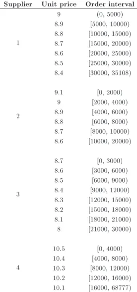
1 (3, 4.04, 4.9) (0.4, 0.44, 0.48) (0.0307, 0.0344, 0.0389) 2 (6, 6.48, 7.12) (0.55, 0.64, 0.67) (0.0498, 0.0551, 0.0674) 3 (7, 7.17, 7.8) (0.71, 0.72, 0.78) (0.0116, 0.0121, 0.0149) 4 (5, 5.87, 6.23) (0.55, 0.57, 0.62) (0.0205, 0.0215, 0.0265) Table 3. Quantity discounts oered by suppliers.
Supplier Unit price Order interval
1
9 (0, 5000)
8.9 [5000, 10000) 8.8 [10000, 15000) 8.7 [15000, 20000) 8.6 [20000, 25000) 8.5 [25000, 30000) 8.4 [30000, 35108)
2
9.1 [0, 2000) 9 [2000, 4000) 8.9 [4000, 6000) 8.8 [6000, 8000) 8.7 [8000, 10000) 8.6 [10000, 20000)
3
8.7 [0, 3000) 8.6 [3000, 6000) 8.5 [6000, 9000) 8.4 [9000, 12000) 8.3 [12000, 15000) 8.2 [15000, 18000) 8.1 [18000, 21000) 8 [21000, 30000)
4
10.5 [0, 4000) 10.4 [4000, 8000) 10.3 [8000, 12000) 10.2 [12000, 16000) 10.1 [16000, 68777)
are also given in Table 2. In addition, the discount price oered by suppliers is shown in Table 3.
Let us denote fuzzy objectives by ]Cost = (1; 2; 3) and ^AP V = (1; 2; 3). According to the
proposed method, we need to determine the interval G; Gfor each objective. For this purpose, two single-objective optimization models are solved for = 0. By minimizing 1, the fuzzy optimal solution is obtained
as ]Cost = (1584200; 1698800; 1819600). Also, by maximizing 3, the fuzzy optimal solution is ^AP V =
(67000; 70000; 75000). Given the optimal solutions to
Table 4. Pareto solutions to the problem with respect to dierent values of .
# K1 K2 K1 K2
1 0.1 0.6358 0.7924 0.0635 0.0792 2 0.1 0.7909 0.1831 0.0790 0.0183 3 0.2 0.6355 0.797 0.1271 0.1594 4 0.2 0.7861 0.2038 0.1572 0.0407 5 0.3 0.5214 0.8016 0.1564 0.2404 6 0.3 0.776 0.223 0.2328 0.0669 7 0.4 0.6815 0.806 0.2726 0.3224 8 0.4 0.7802 0.258 0.3120 0.1032 9 0.5 0.4988 0.8102 0.2494 0.4051 10 0.5 0.7865 0.2828 0.3932 0.1414 11 0.6 0.6538 0.8143 0.3922 0.4885 12 0.6 0.7822 0.3043 0.4693 0.1825 13 0.7 0.6242 0.8183 0.4369 0.5728 14 0.7 0.7806 0.3252 0.5464 0.2276 15 0.8 0.6678 0.8221 0.5342 0.6576 16 0.8 0.7561 0.3218 0.6048 0.2574 17 0.9 0.6785 0.8259 0.6106 0.7433 18 0.9 0.7816 0.3722 0.7034 0.3349 19 1 0.5605 0.8295 0.5605 0.8295 20 1 0.7698 0.3253 0.7698 0.3253
the two optimization models, it is determined that GCost = 1584200 and GAP V = 75000. The DM also
sets the non-ideal values for both objective functions as GCost = 2300000 and GAP V = 55000. Thus, the
interval G; G for cost and APV will be (1584200, 2300000) and (55000, 75000), respectively.
Table 4 shows the Pareto solutions obtained by solving the problem for dierent values of . The problem has been solved for = 0:1; 0:2; :::; 1 and the satisfaction level of the DM has been reported. Also, normalized satisfaction levels are shown in the fth and sixth columns.
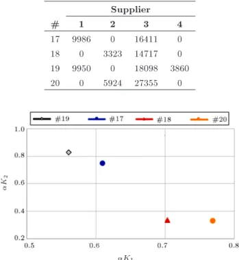
Regarding the normalized satisfaction levels, if the dominated solutions are eliminated, solutions 17{ 20 are identied as the nal Pareto solutions. Figure 5 shows the remaining Pareto solutions.
Table 5 shows the order quantities assigned to suppliers in Pareto solutions. Also, the fuzzy member-ship functions for cost and APV objectives are shown
Table 5. Order quantities in Pareto solutions. Supplier
# 1 2 3 4
17 9986 0 16411 0
18 0 3323 14717 0
19 9950 0 18098 3860
20 0 5924 27355 0
Figure 5. Final Pareto solutions with respect to the normalized satisfaction levels.
Figure 6. Fuzzy membership function of cost objective in Pareto solutions.
in Figures 6 and 7, respectively. According to them, the DM can choose the appropriate solution.
Given the fuzzy values of the cost in Figure 6, we can compare the solutions. According to the calculations of fuzzy cost values: (a) The degrees in which solution #20 is bigger than solutions #17, #18, and #19 are 1, 0.97, and 1, respectively; (b) The degrees in which solution #18 is bigger than solutions #17 and #19 are 0.85 and 0.8, respectively; and (c) The degree in which solution #19 is bigger than solution #17 is 0.55. Given the minimization of the cost objective function, solution #20 is the worst among all the solutions.
Similarly, we can compare the solutions given the fuzzy values of APV objective in Figure 7: (a) There is no dierence between solutions #17 and #19; (b)
Figure 7. Fuzzy membership function of APV objective in Pareto solutions.
Figure 8. Pareto frontiers with regard to dierent values of R.
The degree in which both solutions #18 and #20 are bigger than either solution #17 or #19 is equal to 1; and (c) There is no dierence between solutions #18 and #20. For indierent solutions in APV, one can choose a solution that is more cost-eective.
According to the analysis, there is no dierence between solutions #18 and #20 in APV and the degree in which solution #20 is bigger than #18 is 0.97. Therefore, solution #18 is preferred to solution #20. Similarly, there is no dierence between solutions #17 and #19 in APV and the degree in which solution #19 is bigger than #17 is 0.55. Therefore, solution #17 is preferred to solution #19.
In the example above, the maximum acceptable defective rate (R) is assumed to be 0.022. In the follow-ing, the problem is also solved for R = 0:02; 0:024, and 0.030 and the same procedure is followed to identify the nal Pareto solutions. Figure 8 shows the results. In the maximization of satisfaction levels, the farther the Pareto frontier from the origin, the better the quality of its solutions will be. It is expected that by increasing R, the solution space gets wider and better results are obtained. Figure 8 also conrms this.
7. Conclusion
se-lection is one of the major processes in supply chain management of any organization. On the other hand, allocating orders to the selected suppliers allows for some economies of scale through the right choice of the quantities to order from each supplier. In this paper, the supplier selection and order allocation problem was studied in a single-buyer-multi-supplier supply chain. Suppliers oered quantity discounts as an incentive to motivate buyers to increase the amount of their ordered quantities. Also, transportation cost, fuzzy-type uncertainty, and some practical constraints were taken into account in the problem. The problem was formulated as a bi-objective model to minimize annual supply chain costs and maximize the Annual Purchasing Value (APV). We proposed a novel fuzzy multi-objective programming method based on the degree of satisfaction of the Decision Maker (DM) and the fulllment level of fuzzy constraints. After solving the model and determining Pareto solutions, the fuzzy results were compared with an index and the DM could identify the appropriate or inappropriate solutions. We utilized Non-dominated Sorting Genetic Algorithm (NSGA II) to solve the model and the results were presented using numerical examples. The interested researchers can also investigate demand uncertainty, the eect of dierent potential suppliers in each period, and other quantity discount schemes such as incremen-tal quantity discounts and business volume quantity discounts in the problem. Also, other algorithms such as Multi-Objective Particle Swarm Optimization (MOPSO) and Multi-Objective Simulated Annealing (MOSA) can be applied to the problem in order to investigate the eciency of the proposed NSGA II.
References
1. Hamdan, S. and Cheaitou, A. \Supplier selection and order allocation with green criteria: An MCDM and multi-objective optimization approach", Comput. Oper. Res., 81, pp. 282{304 (2017).
2. Govindan, K., Rajendran, S., Sarkis, J., et al. \Multi criteria decision making approaches for green supplier evaluation and selection: a literature review", J. Clean. Prod., 98, pp. 66{83 (2015).
3. Guo, C. and Li, X. \A multi-echelon inventory system with supplier selection and order allocation under stochastic demand", Int. J. Prod. Econ., 151, pp. 37{ 47 (2014).
4. Kannan, D., Khodaverdi, R., Olfat, L., et al. \Inte-grated fuzzy multi criteria decision making method and multi-objective programming approach for sup-plier selection and order allocation in a green supply chain", J. Clean. Prod., 47, pp. 355{367 (2013).
5. Pazhani, S., Ventura, J.A., and Mendoza, A. \A serial inventory system with supplier selection and order quantity allocation considering transportation costs", Appl. Math. Model., 40(1), pp. 612{634 (2016).
6. Ballou, R.H., Business Logistics Management. Upper Saddle River, NY Prentice Hall (1992).
7. Mansini, R., Savelsbergh, M.W.P., and Tocchella, B. \The supplier selection problem with quantity dis-counts and truckload shipping", Omega, 40(4), pp. 445{455 (2012).
8. Taleizadeh, A.A., Stojkovska, I., and Pentico, D.W. \An economic order quantity model with partial back-ordering and incremental discount", Comput. Indust. Eng., 82, pp. 21{32 (2015).
9. Ayhan, M.B. and Kilic, H.S. \A two stage approach for supplier selection problem in multi-item/multi-supplier environment with quantity discounts", Com-put. Indust. Eng., 85, pp. 1{12 (2015).
10. Jimenez, M., Arenas, M., Bilbao, A., et al. \Linear programming with fuzzy parameters: an interactive method resolution", Eur. J. Oper. Res., 177(3), pp. 1599{1609 (2007).
11. Dahel, N.-E. \Vendor selection and order quantity allocation in volume discount environments", Suppl. Chain Manag.: Int. J., 8(4), pp. 335{342 (2003).
12. Demirtas, E.A. and Ustun, O. \An integrated multi-objective decision making process for supplier selection and order allocation", Omega, 36, pp. 76{90 (2008).
13. Xia, W. and Wu, Z. \Supplier selection with multiple criteria in volume discount environments", Omega, 35(5), pp. 494{504 (2007).
14. Burke, G.J., Carrillo, J., and Vakharia, A.J. \Heuris-tics for sourcing from multiple suppliers with alterna-tive quantity discounts", Eur. J. Oper. Res., 186(1), pp. 317{329 (2008).
15. Kokangul, A. and Susuz, Z. \Integrated analytical hierarch process and mathematical programming to supplier selection problem with quantity discount", Appl. Math. Model., 33(3), pp. 1417{1429 (2009).
16. Amid, A., Ghodsypour, S.H., and O'Brien, C. \A weighted additive fuzzy multiobjective model for the supplier selection problem under price breaks in a supply chain", Int. J. Prod. Econ., 121(2), pp. 323{ 332 (2009).
17. Wang, T.-Y. and Yang, Y.-H. \A fuzzy model for supplier selection in quantity discount environments", Expert Syst. Appl., 36(10), pp. 12179{12187 (2009).
18. Ebrahim, R.M., Razmi, J., and Haleh, H. \Scatter search algorithm for supplier selection and order lot sizing under multiple price discount environment", Adv. Eng. Soft., 40(9), pp. 766{776 (2009).
19. Razmi, J. and Maghool, E. \Multi-item supplier selec-tion and lot-sizing planning under multiple price dis-counts using augmented e-constraint and Tchebyche method", Int. J. Adv. Manuf. Technol., 49(1{4), pp. 379{392 (2010).
20. Kamali, A., Fatemi-Ghomi, S., and Jolai, F. \A multi-objective quantity discount and joint optimization model for coordination of a single-buyer multi-vendor supply chain", Comput. Math. Appl., 62(8), pp. 3251{ 3269 (2011).
21. Zhang, J.L. and Zhang, M.Y. \Supplier selection and purchase problem with xed cost and constrained order quantities under stochastic demand", Int. J. Prod. Econ., 129(1), pp. 1{7 (2011).
22. Lee, A.H.I., Kang, H.-Y., Lai, C.-M., et al. \An integrated model for lot sizing with supplier selection and quantity discounts", Appl. Math. Model., 37(7), pp. 4733{4746 (2013).
23. Moghaddam, K.S. \Fuzzy multi-objective model for supplier selection and order allocation in reverse logis-tics systems under supply and demand uncertainty", Expert Syst. Appl., 42, pp. 6237{6254 (2015).
24. Bohner, C. and Minner, S. \Supplier selection under failure risk, quantity and business volume discounts", Comput. Indust. Eng., 104, pp. 145{155 (2017).
25. Cebi, F. and Otay, _I. \A two-stage fuzzy approach for supplier evaluation and order allocation problem with quantity discounts and lead time", Inf. Sci., 339, pp. 143{157 (2016).
26. Hamdan, S. and Cheaitou, A. \Dynamic green supplier selection and order allocation with quantity discounts and varying supplier availability", Comput. Indust. Eng., 110, pp. 573{589 (2017).
27. Ranjbar Tezenji, F., Mohammadi, M., Pasandideh, S.H.R., et al. \An integrated model for supplier location-selection and order allocation under capacity constraints in an uncertain environment", Sci. Iran., E, 23(6), pp. 3009{3025 (2016).
28. Jimenez, M. and Bilbao, A. \Pareto-optimal solutions in fuzzy multi-objective linear programming", Fuzzy Set. Syst., 160(18), pp. 2714{2721 (2009).
29. Sakawa, M., Fuzzy Sets and Interactive Multiobjec-tive Optimization, Springer Science & Business Media (2013).
30. Tiwari, R.N., Dharmar, S., and Rao, J. R. \Fuzzy goal programming-an additive model", Fuzzy Set. Syst., 24(1), pp. 27{34 (1987).
31. Chen, L.H. and Tsai, F.C. \Fuzzy goal programming with dierent importance and priorities", Eur. J. Oper. Res., 133(3), pp. 548{556 (2001).
32. Wu, Y.K. and Guu, S.M. \A compromise model for solving fuzzy multiple objective linear programming problems", J. Chinese Ins. Indust. Eng., 18(5), pp. 87{93 (2001).
33. Akoz, O. and Petrovic, D. \A fuzzy goal programming method with imprecise goal hierarchy", Eur. J. Oper. Res., 181(3), pp. 1427{1433 (2007).
34. Lee, E.S. and Li, R.J. \Fuzzy multiple objective pro-gramming and compromise propro-gramming with Pareto optimum", Fuzzy Set. Syst., 53(3), pp. 275{288 (1993).
35. Arikan, F. \A fuzzy solution approach for multi objec-tive supplier selection", Expert Syst. Appl., 40(3), pp. 947{952 (2013).
36. Li, X.Q., Zhang, B., and Li, H. \Computing ecient solutions to fuzzy multiple objective linear program-ming problems", Fuzzy Set. Syst., 157(10), pp. 1328{ 1332 (2006).
37. Erginel, N. and Gecer, A. \Fuzzy multi-objective deci-sion model for calibration supplier selection problem", Comput. Indust. Eng., 102, pp. 166{174 (2016).
38. Govindan, K., Darbari, J.D., Agarwal, V., et al. \Fuzzy multi-objective approach for optimal selection of suppliers and transportation decisions in an eco-ecient closed loop supply chain network", J. Clean. Prod., 165, pp. 1598{1619 (2017).
39. Zadeh, L.A. \Fuzzy sets", Inf. Control, 8(3), pp. 338{ 353 (1965).
40. Alaei, S. and Khoshalhan, F. \A hybrid cultural-harmony algorithm for multi-objective supply chain coordination", Sci. Iran. E, 22(3), pp. 1227{1241 (2015).
41. Dubois, D., Kerre, E., Mesiar, R., et al. \Fuzzy interval analysis", In: Dubois, D., Prade, H. (Eds.), Fundamentals of Fuzzy Sets, Kluwer, Massachusetts, pp. 483{561 (2000).
42. Yager, R.R. \Ranking fuzzy subsets over the unit interval", In: Proc. of 17th IEEE Int. Conf. on Dec. Control, San Diego, CA, pp. 1435{1437 (1979).
43. Heilpern, S. \The expected valued of a fuzzy number", Fuzzy Set. Syst., 47, pp. 81{86 (1992).
44. Deb, K., Agrawal, S., Pratap, A., et al. \A fast elitist non-dominated sorting genetic algorithm for multi-objective optimization: NSGA-II", In Int. Conf. on Parallel Prob. Solv. From Nature, pp. 849{858, Springer, Berlin, Heidelberg (2000).
45. Deb, K., Multi-Objective Optimization Using Evolu-tionary Algorithms, 16, John Wiley & Sons (2001).
Biographies
Mohammad Ali Sobhanolahi obtained BSc and MSc degrees in Mathematics from Tabriz University, Tabriz, Iran, in 1973 and 1975, respectively. He also received another MSc degree in Public Management from Tabriz University, Tabriz, Iran, in 1991 and the PhD in Industrial Engineering from Swinburne University, Australia, in 1996. Currently, he is a Professor in the Faculty of Industrial Engineering at Kharazmi University, Tehran, Iran. He has authored numerous papers presented at conferences and pub-lished in national and international journals.
Ahmad Mahmoodzadeh received BSc degree in Manufacturing Engineering from Shahid Rajaee Teacher Training University, Tehran, Iran, in 2000, and MSc degree in Industrial Engineering from Mazandaran
University of Science and Technology, Babol, Iran, in 2003. Currently, he is a PhD candidate in In-dustrial Engineering at Kharazmi University, Tehran, Iran.
Bahman Naderi completed his BSc degree in Indus-trial Engineering at Mazandaran University of Science
and Technology, Babol, Iran; MSc and PhD degrees in the same eld at Amirkabir University of Technology, Tehran, Iran; and post-doctoral program at University of Windsor, Canada. Currently, he is an Assistant Professor at Kharazmi University, Tehran, Iran. His research interest is applied operations research (math-ematical modeling and solution method).