Sharif University of Technology
Scientia IranicaTransactions B: Mechanical Engineering http://scientiairanica.sharif.edu
Closed form solution for direct and inverse kinematics
of a US-RS-RPS 2-DOF parallel robot
J. Sanjuan
, D. Serje, and J. Pacheco
Department of Mechanical Engineering, Universidad del Norte, Km. 5 Via Puerto Colombia, Barranquilla, Colombia. Received 1 October 2016; received in revised form 1 March 2017; accepted 17 July 2017
KEYWORDS Parallel iknematics; Forward kinematics; Pose;
Homogeneous transformation matrix; Closed form.
Abstract. Parallel mechanisms with reduced Degree Of Freedom (DOF) have grown in importance for industry and researchers as they oer a simpler architecture and lower manufacturing/operating costs with great performance. In this paper, a two-degree-of-freedom parallel robot is proposed and analyzed. The robot with a xed base, a moving platform, and three legs achieve translational and rotational motions through actuation on prismatic and revolute joints and can be applied to pick-and-place applications, vehicle simulators, etc. Through homogeneous transformation matrices and Sylvesters dialytic elimination method, a closed-form solution for direct kinematics is obtained for all possible assembly modes. Inverse kinematics is solved by the closed-form solution as well. This greatly decreases computational time, suggesting the optimality of the proposed approach. A case study is investigated to validate the solutions found and is compared with a CAD model to corroborate the obtained results. Finally, a workspace calculation is carried out for dierent geometrical parameters of the robot.
© 2018 Sharif University of Technology. All rights reserved.
1. Introduction
Parallel Kinematic Machines (PKMs), compared to serial robots, oer some useful features such as higher structural rigidity (stiness), kinematic accuracy (non-cumulative joint error), higher payload to robot weight ratio, compactness, and modularity [1-3]. In the past two decades, all of these advantages have won PKMs special reverence for the industry in the elds of machine tooling, high-speed pick-and-place applica-tions, vehicle driving simulators, and solar tracking mechanisms among others. One of the main issues of PKMs is their complex forward kinematics, often implying to nd the solution of nonlinear systems of equations which may not be unique [4] and their
*. Corresponding author.
E-mail address: [email protected] (J. Sanjuan) doi: 10.24200/sci.2017.4341
limited workspace which limits their application in some industry markets [5].
In literature, forward kinematics has received extensive attention. Therefore, many approaches have been proposed, classied into two main classes: nu-merical methods and analytic techniques. Dierent numerical methods have been applied, e.g., neural networks strategies [6], Taylor expansion series with n-order polynomials [7], Newton classical methods [3], and fuzzy inference systems [8]. Although numerical techniques have successfully achieved a fast solution to some problems, their accuracy is dependent on itera-tions required for a good convergence [9]; they fail to describe the set of solutions to the nonlinear equations governing the problem [10]. Other numerical/graphical methods use CAD functionalities to design computer simulation mechanisms of PKMs that can be used to analyze forward kinematics; further, a variation geometry approach is proposed to shape and solve the reachable workspace problem [11].
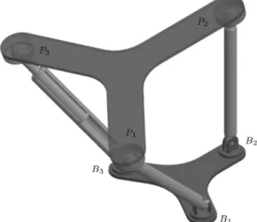
Figure 1. The US-RS-RPS parallel robot.
dierent congurations on PKMs, various analyti-cal techniques have been used for dierent require-ments, e.g., Sylvesters dialytic elimination method on a 3(RSS)-S fully spherical robot [12], homotopy continuation method for a 3-UPU translational parallel robot [13], and Grobner basis for lexicographic ordering of equations for a planar Stewart platform [14]. Al-though analytical strategies lead to the discovery of a closed-form solution, its complexity often requires the use of numerical methods; for instance, Dhingra et al. found a 20th-degree polynomial for the direct kinematics of the Stewart platform [15].
To overcome complex kinematics and control, designers have explored dierent architectures from universal full mobility parallel robots, such as the Gough-Stewart platform, to robots with reduced DOF with a simpler architecture and lower manufactur-ing/operating costs. Although decreasing the DOF re-duces the available workspace, it also lowers complexity on forward kinematics solution, incidence of singular-ities, voids and legs collisions [16] from the tracking space as evidenced by Dunlop et al. [17]. In particular, the two DOF parallel mechanisms have attracted much attention of the designers, and various examples of ap-plications of two spatial and planar DOFs mechanisms can be found in dierent industrial sectors; for instance, Zhang et al. described a 2-DOF mechanism in a vehicle driving simulator [18]; Cammarata designed a 2-DOF mechanism for solar tracking systems [19]; Rico et al. developed a knee rehabilitation device using a planar parallel mechanism [20]. Although there is an increased interest in those mechanisms, there are still many types that have not been analyzed.
This paper studies a US-RS-RPS parallel robot, which is a 2-DOF parallel robot with translational and rotational capabilities (shown in Figure 1). This architecture oers simple kinematic actuation on pris-matic and revolute joints and can be used on pick-and-place applications, simple vehicle driving
simu-lators, solar tracking mechanisms or others accord-ing to users' requirements. The position analysis of this mechanism is carried out using homogeneous transformation matrices. These matrices are mainly used for analysis of serial mechanisms, allowing for an intuitive understanding of the relationship between passive and active joints and the position and orienta-tions of moving platform [21]. A closed-form solution for all congurations is achieved using the Sylvesters dialytic elimination method. Inverse kinematics is also analyzed; nally, a case study is shown with a symmet-ric structure exhibiting four real congurations, and the workspace calculated is also done for illustration purposes.
2. Description of the US-RS-RPS parallel robot
The US-RS-RPS parallel robot is composed of a moving platform (P1; P2; P3), a xed base (B1; B2; B3), and
three legs (B1P1; B2P2; B3P3) (see Figures 1 and 2).
Leg one has a universal (U) joint (passive) attached to the base and is attached to the moving platform by a spherical (S) joint; the universal joint is described by angles and . Leg two has an actuated revolute (R) joint assembled to the base and a spherical (S) joint attached to the moving platform; angle describes the revolute joint. Leg three has a revolute (R) joint connected to the base, an actuated prismatic (P) joint, and a spherical joint connected to the moving platform; angle describes the revolute joint and describes the prismatic actuation as an expansion/contraction of the leg's initial length. The length of the legs is dened by L.
Each leg is attached to the base at points Bi
and to the moving platform at points Pi, as shown
in Figures 2 and 3. Reference coordinate system xyz, is attached to the center of the xed base, O. Bi points are referenced to coordinate system xyz
through a translation in z axis described by distance d followed by a rotation along x axis, measured through angle i. The orientation of the moving platform is
represented by coordinate system uvw which is located at the center of the moving platform at point Op. Pi
points are referenced to the coordinate system uvw through a translation in w axis described by distance a followed by a rotation along u axis, measured through angle i. Coordinate system uvw and its position
are described by homogeneous transformation matrix MOp
O . Coordinate system uvw is dened by roll, pitch
and yaw angle parameters, namely a rotation of x
about xed x axis, followed by rotation y about xed
y axis, and rotation zabout xed z axis. There is no
particular reason for selecting such a denition. Thus, matrix MOp
O can be expressed by Eq. (1) as shown in
MOp
O =
2 6 6 4
cycz cysz sy Ox
cxsz+ czsxsy cxcz sxsysz cysx Oy
sxsz cxczsy czsx+ cxsysz cxcy Oz
0 0 0 1
3 7 7
5 : (1)
Box I
Figure 2. Schematic diagram of the parallel manipulator.
cos() and sin() are represented by c() and s(). Eq. (1) is written in terms of the unit vectors uvw attached to platform and its origin as follows:
MOp
O =
!u !v !w O!
p
0 0 0 1
: (2)
The center of the moving platform can be repre-sented as a function of Pipoints through the barycenter
equation: ! Op= 13
3
X
i=1
Pi: (3)
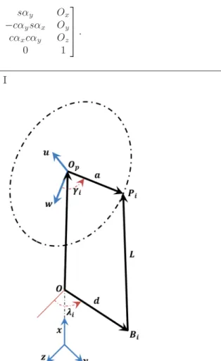
Figure 3. Geometry of a general kinematic chain.
Considering that the direction of unit vector !w is along vectorOpP!3, the direction of unit vector !u is
perpendicular to the moving platform, and unit vector !v is perpendicular to unit vectors !u and !w , then Eq. (2) is written in terms of Pi points as shown in
Box II. Using the results from Eqs. (2) and (4), the rotation angles of Eq. (1) can be found in terms of Pi
points using the relationship shown below: y = a tan 2
u2
x+ vx2
1 2; w
x
; (5)
z= a tan 2
vx
cy;
ux
cy
; (6)
MOp
O =
2 6 6 4
!
OpPiOpPi+1!
OpP!1OpP!2
! OpP3
~
OpPiOpPi+1!
OpP!1OpP!2
! OpP3
OpP!3
! Op
0 0 0 1
3 7 7
5 : (4)
x= a tan 2
wx
cy ;
wz
cy
: (7)
Finally, the DOFs of the US-RS-RPS parallel robot are calculated using both the Grubler-Kutzbach equation as used in [22] and the analytical DOF method of an end eector using reciprocal screw theory is depicted in [23]. First, using the Grubler-Kutzbach yields:
M = (L 1)
g
X
i=1
fi= 6 (7 1) 34 = 2; (8)
where L represents the number of links, represents the task space, fi denotes the DOF of joint i, and g
represents the number of joints. The coordinate system attached to the center of the moving platform can be oriented and displaced by the actuation of prismatic joint, , and revolute joint, .
The second approach calculates twist ($i) of each
leg of the platform and uses these results to compute the wrench ($r
i) of each leg through the reciprocal
screws formula presented below:
$i $ri = 0: (9)
The wrenches obtained are grouped in matrix $r,
and the DOFs of the mechanism are solved using again the reciprocal screws formula, only this time to obtain the value of $F as shown below:
$F $r
i = 0: (10)
The non-zero rows of matrix $F represent the
DOF of the mechanism; for the case of the US-RS-RPS parallel robot, the analyses are carried out obtaining two rows for matrix $F, and then the mechanism has
two DOFs.
3. Direct kinematic analysis
The US-RS-RPS parallel robot, as mentioned before, has two DOFs, assuming that the actuation falls on prismatic () and revolute joint on the second leg (). There are still three passive joints which need to be solved in order to solve the direct kinematic problem; these passive joints are ; , and .
To solve the direct kinematics primarily, coupling points, Bi, are obtained using two transformations.
First, considering a rotation in the direction of x axis by angle i and a displacement in z axis by distance
d, these two transformations yield the homogeneous transformation matrix shown below:
TBi =
2 6 6 4
1 0 0 0
0 ci si dsi
0 si ci dci
0 0 0 1
3 7 7 5
=!xl !yl !zl B!i
0 0 0 1
; (11)
where !xi; !yi; and !zi are the directions of the coordinate
system attached to point Bi.
Furthermore, according to the representation shown in Figure 3, the position equation associated with Pi points can be dened in two ways as shown
in the following equations:
Pi= Op+ OpPi; (12)
Pi= Bi+ BiPi: (13)
These equations can also be stated in terms of the homogeneous transformation matrix. For Eq. (12), the position of Op is obtained using the homogeneous
transformation matrix, MOp
O ; additionally, position
vector Op!Pi is determined by two transformations: a
rotation in the direction of u axis by angle i, and a
displacement in \the rotated" w axis by distance a, obtaining subsequent equivalence for Pi:
Pi=
2 4OOxy
Oz
3 5
+ 2
4 asi(cxacczissy+ acxsysysz) aczsi ycisx acxcyci asi(czsx+ cxsysz)
3 5 :
(14) Besides, the solution to Eq. (15) is achieved by suc-cessive transformations through the axis of each joint linked to every arm of the mechanism generating the coordinates of every Pipoint in the robot. As depicted
below: P1=
2
4L (c1s + csLcc1s) ds1 L (s1s cc1s) + dc1
3
5 ; (15)
P2=
2
4 s2(d Ls)Lc c2(d Ls)
3
5 ; (16)
P3=
2
4 s3Lc (d Ls ) c3(d Ls )
3
5 : (17)
Using the results of Eqs. (15), (16), and (17), the next three equations express the distance of segments P1P2, P2P3, and P1P3, respectively:
K5+ K6c + K7s = 0; (19)
K8+ K9cs + K10cc + K11s = 0; (20)
where terms K1 to K7 are dependent on geometric
parameters (dimensions), d, L1, P1P2, P2P3, P1P3,
1, 2, 3, and active joints, and ; terms K8 to
K11 are functions of and the mentioned parameters.
The detailed expressions for K1 to K11 terms are
given in the Appendix. Eq. (19) relates passive joint with active joint implicitly; to explicitly solve this equation for , an half-angle substitution is used, resulting in:
= 2 tan 1 K7
p K2
7 K52+ K62
K5 K6
!
: (21)
Using the results of on Eqs. (18) and (20) and performing another half angle substitution for angle on both equations yield:
K12T2+ K13T+ K14= 0; (22)
K15T2+ K16T+ K17= 0; (23)
where T stands for half angle substitution, T =
tan(=2); similarly, for Eq. (21), coecients K12to K17
are functions of the mentioned geometric parameters, active joints and and passive joints and . The detailed expressions for K12 to K17 coecients are
given in the Appendix. The coecients of Eqs. (22) and (23) are used to create the matrix shown below:
S = 2 6 6 4
0 K12 K13 K14
K12 K13 K14 0
0 K15 K16 K17
K15 K16 K17 0
3 7 7
5 : (24)
For this matrix, if T is a solution to Eqs. (22) and
(23), then coecients K12; K13, and K14 are linear to
K15; K16, and K17; as a consequence, the determinant
of matrix S must be equal to zero, which produces the equation below:
det(S) =K2
12K172 K12K13K16K17
2K12K14K15K17+ K12K14K162
+ K2
13K15K17 K13K14K15K16
+ K2
14K152 = 0: (25)
As mentioned, coecients K12 to K17 are functions
of already known parameters, except for , which is the only unknown parameter in this equation. To solve Eq. (18) for , another half angle substitution is carried out, yielding the next quartic function:
K18T4+ K19T3+ K20T2+ K21T+ K22= 0; (26)
where T represents half angle substitution T =
tan(=2). Coecients K18 to K22 are described in
detail in the Appendix. Eq. (26) has four solutions and many analytical methods exist to solve it [24]. Once a solution for is obtained, it is easy to solve using one of Eqs. (22) and (23) and substituting T= tan(=2).
Using Eq. (22) yields:
= 2 tan 1 K13pK132 4K12K14
2K12
!
: (27)
Once the passive joints are explicitly solved, the direct kinematic is obtained in a straightforward way, as every coupling point of the platform is a function of the passive and active joints as depicted in Eqs. (15) to (17). Then, as described in Eqs. (3) to (7), the position and orientation of the moving platform is also found as these equations are functions of the coupling points. 4. Inverse kinematics
The inverse kinematic problem focuses on the solution of the active joints position, knowing the position and orientation of the moving platform. As mentioned before, the position and orientation of the moving platform are described by Eq. (1). Moreover, Eq. (15) describes the position of Pi points as a function of the
orientation and the position of the moving platform. Using these results, the inverse kinematic problem is solved obtaining the values of actives joints, and , as functions of points P1, P2, and P3.
Employing the expression for x coordinate of point P2 and dividing it by the expression for y
coordinate of point P2 easily yield the expression for
active joint : = tan 1
P2y+ ds2
s2P2x
: (28)
To nd the solution for active joint initially, it is needed to solve the passive joint, . Using a similar procedure rather than the used one to nd , is found using the expression for x coordinate of point P3 and
the expression for y coordinate of point P3, producing:
= tan 1P3y+ ds3
P3x
: (29)
At last, the solution for active joint is found in a straightforward way replacing the obtained value in Eq. (22) in the expression for z coordinate of point P3,
generating: = c3Ld P3
1s : (30)
Eqs. (14), (28), (29), and (30) solve the inverse kinematic for the US-RS-RPS parallel robot.
5. Case study
In this section, an example of a solution to direct kinematic problem of the US-RS-RPS parallel robot is presented. For this purpose, the constant geo-metric parameters (d; L1; a; 1; 2; 3) and position of
the actuators (; ) are supplied. The solution will determine the position of the coupling points of the platform (P1; P2; P3) by obtaining three angles ; ,
and . Afterwards, in order to validate the solution, the direct kinematic solution is used as an input to the inverse kinematic model.
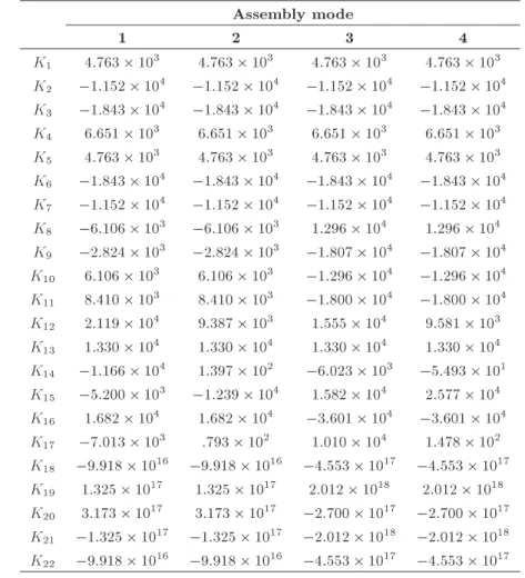
The architecture parameters and actuation values are shown in Table 1. Ki coecients used to solve the
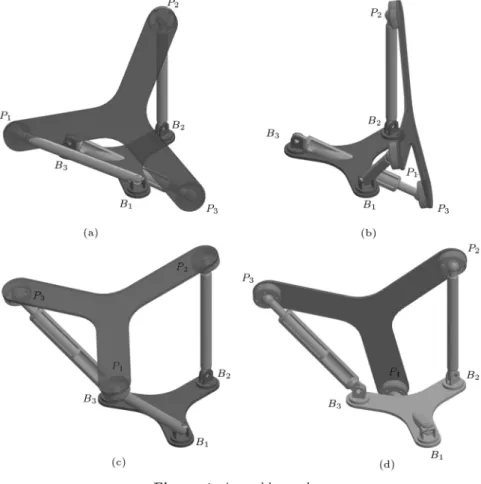
forward kinematic problem are also depicted for every solution (assembly modes) in Table 2. Using these values, passive joints ; , and are calculated, the values are listed in Table 3, and the coupling points (P1; P2; P3) are also listed in Table 3. These parameters
show the particular solution for each assembly mode. According to these results, the solutions are shown graphically in Figure 4.
Validation of the proposed model is made using the coupling points as inputs for the inverse kinematic model, and then the actives joints are obtained, as shown in Table 4. The results corroborate the accuracy
of the proposed model for the direct position analysis of the manipulator. This is also veried through a com-parison with a 3D CAD model developed with proper constraints and dimensions to solve the kinematic parameters of the platform, achieving the same results from the proposed closed-form solution [25]. Figure 5 shows an example CAD model used for assembly mode 3 evaluation.
6. Workspace calculation
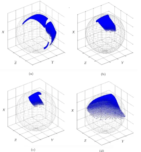
For the current case study, only theoretical workspace is considered and calculated using the solution obtained by forward kinematics [26]. For assembly mode C (see Figure 4), with applied geometrical and joint con-straints, workspace is calculated as a radial projection of platform center on a sphere in Cartesian space, as shown in Figure 6. By using a projected workspace, translational and rotational capabilities of manipulator can be seen in one graph. As stated before, robot conguration and dimensioning is crucial; therefore, dierent topologies and characteristics can be achieved through variations on geometrical parameters. In Figure 6(a), the dimensions of the robot are used for the case of study, and this conguration yields a non-continuous workspace divided into three zones,
Table 1. Input data for the US-RS-RPS parallel robot case study.
d (mm) L (mm) a (mm) 1 and 1 2 and 2 3 and 3
40 96 78:46 120 120 0 0 1
Table 2. Coecients Ki for all assembly modes.
Assembly mode
1 2 3 4
K1 4:763 103 4:763 103 4:763 103 4:763 103
K2 1:152 104 1:152 104 1:152 104 1:152 104
K3 1:843 104 1:843 104 1:843 104 1:843 104
K4 6:651 103 6:651 103 6:651 103 6:651 103
K5 4:763 103 4:763 103 4:763 103 4:763 103
K6 1:843 104 1:843 104 1:843 104 1:843 104
K7 1:152 104 1:152 104 1:152 104 1:152 104
K8 6:106 103 6:106 103 1:296 104 1:296 104
K9 2:824 103 2:824 103 1:807 104 1:807 104
K10 6:106 103 6:106 103 1:296 104 1:296 104
K11 8:410 103 8:410 103 1:800 104 1:800 104
K12 2:119 104 9:387 103 1:555 104 9:581 103
K13 1:330 104 1:330 104 1:330 104 1:330 104
K14 1:166 104 1:397 102 6:023 103 5:493 101
K15 5:200 103 1:239 104 1:582 104 2:577 104
K16 1:682 104 1:682 104 3:601 104 3:601 104
K17 7:013 103 :793 102 1:010 104 1:478 102
K18 9:918 1016 9:918 1016 4:553 1017 4:553 1017
K19 1:325 1017 1:325 1017 2:012 1018 2:012 1018
K20 3:173 1017 3:173 1017 2:700 1017 2:700 1017
K21 1:325 1017 1:325 1017 2:012 1018 2:012 1018
K22 9:918 1016 9:918 1016 4:553 1017 4:553 1017
Table 3. Solutions of the case study.
A. mode ' P1 P2 P3
1 109:349 72:92 52:363
2 6 4 17:22 24:12 73:856 3 7 5 2 6 4 96 34:641 20 3 7 5 2 6 4 31:804 0 50:579 3 7 5
2 109:349 45:710 1:215
2 6 4 67:02 93:13 56:112 3 7 5 2 6 4 96 34:641 20 3 7 5 2 6 4 31:804 0 50:579 3 7 5
3 45:338 28:241 36:263
2 6 4 68:191 94:75 10:86 3 7 5 2 6 4 96 34:641 20 3 7 5 2 6 4 67:483 0 108:28 3 7 5
4 45:338 109:2 0:469
2 6 4 31:57 43:48 26:01 3 7 5 2 6 4 96 34:641 20 3 7 5 2 6 4 67:483 0 108:28 3 7 5
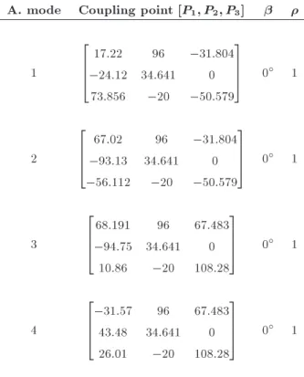
Table 4. Solutions of the inverse kinematics problem for the assembly modes. A. mode Coupling point [P1; P2; P3]
1
2 6 6 4
17:22 96 31:804 24:12 34:641 0 73:856 20 50:579
3 7 7
5 0 1
2
2 6 6 4
67:02 96 31:804 93:13 34:641 0 56:112 20 50:579
3 7 7
5 0 1
3
2 6 6 4
68:191 96 67:483 94:75 34:641 0 10:86 20 108:28
3 7 7
5 0 1
4
2 6 6 4
31:57 96 67:483 43:48 34:641 0 26:01 20 108:28
3 7 7
5 0 1
Figure 5. CAD model for geometry variation.
ing that the robot is limited to one of the three zones. In Figure 6(b), the dimensions of the base platform are increased to become equal to the moving platform maintaining the same lengths of the legs; the result is a small zone above the sphere. In Figure 6(c), the dimensions of the base platform are slightly increased to become bigger than those of the moving platform. As a result, the workspace obtained is smaller than that in the previous conguration. In Figure 6(d),
the dimensions of the base and moving platforms are the same as in the case of study; however the lengths of the legs are heavily increased, obtaining a bigger continuous workspace, almost 1=8 of the total volume of the sphere. The results show that the workspace is highly sensitive to the changes of the dimensions of the robot; thus, it is encouraged to make an optimization process on the robot to obtain the bigger continuous workspace possible.
7. Conclusion
A novel US-RS-RPS 2-DOF parallel robot was pre-sented for dierent applications with positioning and orientation requirements with a simple actuation. The robot structure as well as the coordinate frames were described, and its kinematic was shown as a combi-nation of translation and rotation. Forward kinemat-ics were solved using the homogeneous transforma-tion matrices and geometrical constraints on moving platform achieving a closed form solution. The use of homogeneous transformation matrices was demon-strated to be a useful and intuitive tool to develop the kinematic of parallel robots, because every member can be analyzed as an open kinematic chain that can be further constrained. The system of equation was solved using the Sylvesters dialytic elimination method and a fourth-degree polynomial was found (representing four possible assembly modes). Inverse
Figure 6. Projected workspace for dierent dimensions: (a) L = 96 mm d = 40 mm a = 78:5 mm (case study), (b) L = 96 mm d = 58 mm a = 58 mm (base equal to moving platform), (c) L = 100 mm d = 69 mm a = 58 mm (base bigger than moving platform), and (d) L = 288 mm d = 40 mm a = 78:5 mm (legs dimensions increased).
kinematics was also solved in a straightforward way using matrix homogeneous matrices. A case study was also developed; a comparison of results for direct and inverse kinematics with those of a 3D CAD model shows the eectiveness of the proposed model. Finally, workspace calculation was performed with respect to dierent geometrical parameters, and showing that the systems workspace is highly inuenced by each parameter and conguration.
Future works may extend the current results to the exploration of reconguration capabilities based on possible assembly modes to maximize workspace, condition index, and dynamic performance among others, according to user's needs.
References
1. Fassi, I. and Wiens, G.J. \Multiaxis machining: PKMs and traditional machining centers", Journal of Manu-facturing Processes, 2, pp. 1-14 (2000).
2. Taghirad, H.D., Parallel Robots: Mechanics and Con-trol, CRC Press (2013).
3. Merlet, J.-P., Parallel Robots, Springer, Netherlands (2006).
4. Merlet, J.-P. \Direct kinematics of parallel manipu-lators", IEEE Transactions on Robotics and Automa-tion, 9, pp. 842-846 (1993).
5. Bonev, I., Ilian A., and Gosselin, C.M. \Analytical de-termination of the workspace of symmetrical spherical parallel mechanisms", IEEE Transactions on Robotics, 22, pp. 1011-1017 (2006).
6. Sadjadian, H., Member, H.T., and Fatehi, A. \Neural networks approaches for computing the forward kine-matics of a redundant parallel manipulator", Interna-tional Journal of Computer, Electrical, Automation, Control and Information Engineering, 2, pp. 1664-1671 (2008).
7. Sadjadian, H. and Taghirad, H. \Comparison of dier-ent methods for computing the forward kinematics of a redundant parallel manipulator", Journal of Intelligent and Robotic Systems: Theory and Applications, 44, pp. 225-246 (2005).
8. Jamwal, P.K., Xie, S.Q., Tsoi, Y.H., and Aw, K.C. \Forward kinematics modelling of a parallel ankle rehabilitation robot using modied fuzzy inference",
Mechanism and Machine Theory, 45, pp. 1537-1554 (2010).
9. Uchida, T. and McPhee, J. \Using Grobner bases to generate ecient kinematic solutions for the dynamic simulation of multi-loop mechanisms", Mechanism and Machine Theory, 52, pp. 144-157 (2012).
10. Abbasnejad, G., Daniali, H.M., and Fathi, A. \Closed form solution for direct kinematics of a 4PUS 1PS parallel manipulator", Scientia Iranica, 19, pp. 320-326 (2012).
11. Lu, Y., Shi, Y., and Hu, B. \Solving reachable workspace of some parallel manipulators by computer-aided design variation geometry", Proceedings of the Institution of Mechanical Engineers, 222, pp. 1773-1782 (2008).
12. Enferadi, J. and Shahi, A. \On the position analysis of a new spherical parallel robot with orientation applications", Robotics and Computer-Integrated Man-ufacturing, 37, pp. 151-161 (2016).
13. Varedi, S.M., Daniali, H.M., and Ganji, D.D. \Kine-matics of an oset 3-UPU translational parallel ma-nipulator by the homotopy continuation method", Nonlinear Analysis: Real World Applications, 10, pp. 1767-1774 (2009).
14. Huang, X.H.X. and He, G.H.G. \New and ecient method for the direct kinematic solution of the general planar Stewart platform", IEEE International Con-ference on Automation and Logistics, pp. 1979-1983 (2009).
15. Dhingra, A.K., Almadi, A.N., and Kohli, D. \A Grobner-Sylvester hybrid method for closed-form dis-placement analysis of mechanisms", Journal of Me-chanical Design, 122, pp. 431-438 (2000).
16. Dash, A.K., Chen, I.M., Yeo, S.H., and Yang, G. \Workspace generation and planning singularity-free path for parallel manipulators", Mechanism and Ma-chine Theory, 40, pp. 776-805 (2005).
17. Dunlop, G.R. and Jones, T.P. \Position analysis of a two DOF parallel mechanism
the Canterbury tracker", Mechanism and Machine Theory, 34, pp. 599-614 (1999).18. Zhang, C. and Zhang, L. \Kinematics analysis and workspace investigation of a novel 2-DOF parallel manipulator applied in vehicle driving simulator", Robotics and Computer-Integrated Manufacturing, 29, pp. 113-120 (2013).
19. Cammarata, A. \Optimized design of a large-workspace 2-DOF parallel robot for solar tracking systems", Mechanism and Machine Theory, 83, pp. 175-186 (2015).
20. Chaparro-Rico, B. and Castillo-Castaneda, E. \Design of a 2DOF parallel mechanism to assist therapies for knee rehabilitation", Ingeniera e Investigacion, 36, pp. 98-104 (2016).
21. Kucuk, S. and Bingul, Z. \Inverse kinematics solutions for industrial robot manipulators with oset wrists", Applied Mathematical Modelling, 38, pp. 1983-1999 (2014).
22. Zhao, J.-S., Zhou, K., and Feng, Z.-J. \A theory of degrees of freedom for mechanisms", Mechanism and Machine Theory, 39, pp. 621-643 (2004).
23. Zhao, J.-S., Feng, Z.-J., and Dong, J.-X. \Computa-tion of the congura\Computa-tion degree of freedom of a spatial parallel mechanism by using reciprocal screw theory", Mechanism and Machine Theory, 41, pp. 1486-1504 (2006).
24. Shmakov, S.L. \A universal method of solving quartic equations", International Journal of Pure and Applied Mathematics, 71, pp. 251-259 (2011).
25. Lu, Y. \Using CAD functionalities for the kinematics analysis of spatial parallel manipulators with 3-, 4-, 5-, 6-linearly driven limbs", Mechanism and Machine Theory, 39, pp. 41-60 (2004).
26. Lukanin, V. \Inverse Kinematics, Forward Kinematics and working space determination of 3DOF parallel manipulator with SPR Joint Structure", Periodica Polytechnica, 49, pp. 39-61 (2005).
Appendix
Detailed expressions for K1 to K11 of Eqs. (9), (10)
and (11) are as follows:
K1= 2L2 (P1P2)2+ 2d(d Ls)(1 c(1 2));
K2= 2L(d dc(1 2) + Lsc(1 2));
K3= 2L2c;
K4= 2Ls(1 2)(d Ls);
K5=L2(1 + 2) + 2d(d Ls)(1 c(2 3))
(P2P3)2;
K6= 2L2c;
K7= 2L(d dc(2 3) + Lsc(2 3));
K8=L2 (P1P3)2+ 2d2(1 c(1 3)) + 2L2
K9= 2L(d dc(1 3) + ls(1 3+ )=2
Ls(1 3 )=2);
K10= 2L2c ;
K11= 2Ls(1 3)(d Ls ):
Detailed expressions for K12to K17of Eq. (13) and (14)
are as follows:
K12= K1 (K2s + K3c);
K13= 2K4;
K14= K1+ (K2s + K3c);
K15= K8 (K9s + K10c);
K16= 2K11;
K17= K8+ (K9s + K10c):
Detailed expressions for K18 to K22 of Eq. (17) are as
follows:
K18= W1+ W2;
K19= 4 W4;
K20= 2W1 2W2+ 4W3;
K21= 4W4;
K22= W1+ W2;
where the Wi coecients are described below:
W1= 4(K1K11 K4K8)2;
W2= 4(K1K10 K3K8+ K3K11 K4K10)
(K1K10 K3K8 K3K11 + K4K9);
W3=4(K1K9 K2K8+ K2K11 K4K9)
(K1K9 K2K8 K2K11+ K4K10);
W4=4(K2K3K82 K2K3K112 + K12K9K10
K2
4K9K10 K1K2K8K10 K1K3K8K9
+ K2K4K10K11+ K3K4K9K11):
Biographies
Javier Sanjuan acquired BS and MS degrees in Mechanical Engineering from Universidad del Norte, Barranquilla, Colombia in 2012 and 2016, respectively. At present, he is pursuing a scholarship to continue his studies in the eld of robotics and control. His main research interests are parallel robots dynamics, design and control.
David Serje Martnez received BS and MS degrees in Mechanical Engineering from Universidad del Norte, Barranquilla, Colombia in 2009 and 2010, respectively. Currently, he is pursuing a PhD degree from the same university thanks to a research grant from Colciencias PhD National Scholarship. His main research interest are design engineering, machinery modelling and sim-ulation and micro-machining.
Jovanny Pacheco is currently an Assistant Professor in Mechanical Engineering Department in Universidad del Norte (Barranquilla-Colombia). He received his BS degree in Mechanical Engineering in 1998 and also an MSc degree in 2003 in Mechanical Engineering from Universidad del Norte. He also received his PhD degree in Engineering Science from ITESM, Monterrey Mexico. His current research interests are dynamics and synthesis of parallel mechanism, robotics, and micro machining.