A Weighted Soft-Max PNLMS Algorithm for
Sparse System Identification
M. Bekrani
Department of electrical and computer engineering Qom University of Technology
Qom, Iran [email protected]
H. Zayyani
Department of electrical and computer engineering Qom University of Technology
Qom, Iran [email protected] Received: February 14, 2016- Accepted: June 22, 2016
Abstract—This paper presents a new Proportionate Normalized Least Mean Square (PNLMS) adaptive algorithm
using a soft maximum operator for sparse system identification. To provide a high rate of convergence, soft maximum operator is employed along with a weighting factor, which is proportional to an estimation of output mean square error (MSE). Simulation results show the superiority of the proposed algorithm over its PNLMS-based counterparts.
Keywords-Sparse adaptive filter, System identification, Echo cancelation, Soft maximum.
I. INTRODUCTION
In the last two decades, adaptive filters have achieved wide applications in many signal processing areas [1]. One important area is sparse system identification, which is employed in many applications including channel estimation [2], [3], echo cancelation [4], [5]. In a sparse system, only a few coefficients of the impulse response are active (non-zero) and many of its coefficients are almost inactive (zero or near zero).
In the identification of sparse systems, conventional adaptive filters could be improved, so that the convergence rate is increased while the computational load even decreases. To this end, sparse adaptive filters have been proposed to exploit the sparsity of the filter coefficients [6], [7], [8]. As a special case, the Normalized Least Mean Square (NLMS) adaptive algorithm which employs a unique step-size for all filter coefficients has a slow convergence rate in identification of sparse impulse responses. To mitigate such deficiency, the
Proportionate NLMS (PNLMS) algorithm has been proposed which updates each filter coefficient individually proportional to its magnitude [9]. In addition, some other proportionate adaptive algorithms have been suggested to further improve the performance of NLMS. One of such algorithms is Improved PNLMS (IPNLMS) which employs a combination of proportionate and non-proportionate updating [4], [10]. Moreover, in [11], a µ-law PNLMS (MPNLMS) algorithm has been proposed which calculates an approximation of optimal proportionate step-size.
Another variant of PNLMS algorithm, so-called Individual Activation Factor PNLMS (IAF-PNLMS), employs an individual activation factor for each adaptive filter coefficient, as opposed to a global activation factor in the standard PNLMS algorithm [12]. The IAF-PNLMS algorithm achieves a better distribution of the adaptation energy over the filter coefficients than the standard PNLMS does. Thereby, for systems exhibiting high sparseness, this approach achieves faster convergence, outperforming both the
PNLMS and IPNLMS algorithms
.
A different class of PNLMS algorithms has also been suggested in [13] which takes into account the sparseness measure of the estimated impulse response via a modified coefficient update function and adapts dynamically to the level of sparseness using a new sparseness-controlled approach.In the weight update process, on the other hand, one can exploit sparsity with a sparsity promoting regularization term [14-16]. The method in [14] is based on minimizing a regularized MSE criterion. The proposed method in [15] employs a
l
0 norm in combination with Least Mean Square (LMS) algorithm which results in an improved version of LMS, so-calledl
0-LMS. Moreover,l
0norm sparsity promoting regularization term was employed with PNLMS algorithm in [16].In addition to
l
0norm,l
1norm penalty has also been utilized in conjunction with PNLMS to improve both convergence speed and excess MSE of adaptive filter [17]. Besides, the relation between basis pursuit (1
l
norm optimization) and NLMS algorithm has been investigated in [18] which lead to a new version of PNLMS. Recently, a non-uniform norm (p
norm like) constraint LMS algorithm has also been proposed [19]. Differently, Maximum a Posteriori (MAP) estimation formulation permits the study of a number of prior distributions which naturally incorporate the sparse property of filter coefficients [7]. Consequently, a MAP-LMS adaptive filter [7] and further, a compressed sensing block based MAP-LMS have been introduced [20].The convergence speed of the PNLMS algorithm, though very high initially, however, slows down at a later stage, even becoming worse than NLMS. In [25_], this problem is addressed by introducing a penalty of constructed l1 norm of the coefficients in the PNLMS cost function which favors sparsity. This helps in the shrinkage of the coefficients, especially the inactive taps, thereby arresting the slowing down of convergence.
In [21], a family of block-sparse PNLMS adaptive algorithms is proposed that improve the performance of identifying block-sparse systems. They are based on the optimization of a mixed norm of the adaptive filter’s coefficients.
In this paper, in order to increase the convergence rate of PNLMS, we modify the standard PNLMS algorithm. To do this, a weighted soft maximum operator is introduced and employed instead of a hard maximum operator. The motivation behind this idea is to consider the effect of coefficients in the whole duration of convergence, especially for iterations in which some coefficients are less than the predefined activation thresholds. This procedure improves the performance of the PNLMS algorithm.
We further weight the terms in the soft maximum so that the weighting factor is decreased throughout the convergence of algorithm. The decreasing of the weighting factor is linearly proportional to the
estimated MSE. Finally, we show the superiority of our proposed algorithm using numerical simulations.
II. FAMILY OF PNLMS ADAPTIVE FILTERS Suppose the input signal at discrete time index
n
is
x
(
n
)
and sparse impulse response of the unknown system isw
o
[
w
o,0,
w
o,1,...,
w
o,N1]
T whereN
is the length of the impulse response. As a result, the system output is)
(
)
(
n
n
y
w
Tox
(1)where
x
(
n
)
x
(
n
),
x
(
n
1
),...,
x
(
n
N
1
)
T is the tap-input vector. Moreover, the desired signal is)
(
)
(
)
(
n
y
n
v
n
d
wherev
(
n
)
is themeasurement noise. The noise
v
(
n
)
is assumed to be a zero-mean white Gaussian noise with variance
v2 and uncorrelated with the input signal. The error signal is defined as)
(
)
(
)
(
)
(
n
d
n
n
n
e
w
Tx
(2)where
w
(
n
)
[
w
0(
n
),
w
1(
n
),...,
w
N1(
n
)]
T is theestimated impulse response at time index
n
.A wide range of adaptive filter algorithms, including PNLMS, employs the following update
formula [4]:
)
(
)
(
)
(
)
(
)
(
)
(
)
(
)
1
(
n
n
n
n
n
e
n
n
n
Tx
G
x
x
G
w
w
(3)where
G
(
n
)
diag
{
g
0(
n
),
g
1(
n
),...,
g
N1(
n
)}
is the gain matrix,
0
is the step-size parameter that control the convergence rate of the algorithm, and0
is a regularization parameter that prevents the division by zero.Equation (3) is a recursive equation derived using minimization of a cost function which leads to the minimization of the estimated MSE [27, 28]. To conduct the weight update, an initialize for
w
(
n
0
)
is required, e. g.
w
(
0
)
0
N1. Then (3) is repeated to some stepsn
which is typically large, so that the estimated MSE converges to a steady state. The main idea of the proportionate updating is to assign different step sizes to different coefficients based on their optimal magnitudes. The bigger the magnitude, the larger the step-size assigned [26]. The diagonal elements of gain matrix determine the individual step-sizes of each filter coefficient.For the standard NLMS algorithm,
G
(
n
)
I
NN, which means all active and inactive coefficients have the same step-size. As a result, a slow convergence rate can be achieved in identification of sparse systems. In contrast, the active coefficients of PNLMS have larger step-sizes than inactive coefficients, to achieve a faster convergence. In the following, we describe a variety of the PNLMS algorithms in detailFigure 1: Values of weighted soft-max operator in terms of
0 0.2 0.4 0.6 0.8 1
0 0.5 1 1.5 2 2.5 3 3.5
M
a
g
n
it
u
d
e
y (maximum)
x (minimum)
softmax(x,y),
=0.5 softmax(x,y),
0 1
and then we will propose a new PNLMS adaptive filter.
A. Standard PNLMS
In the standard PNLMS algorithm, the gain elements are defined as [12]
Ni i i i
n
n
n
g
1
)
(
)
(
)
(
(4)
where
i
0
,
1
,
...,
N
1
and
i(
n
)
is the proportionality function which is|)
)
(
|
),
(
max(
)
(
n
f
n
w
in
i
(5)and
f
(
n
)
is the activation factor defined as)
||
)
(
||
,
max(
)
(
n
n
f
w
(6)in which
||
w
(
n
)
||
,
, and
are infinity norm, activation parameter, and initialization parameter, respectively [12]. Parameter
permits starting the adaptation atn
0
when all filter coefficients are initialized to zero [12]. Parameter
prevents an individual coefficient from freezing when its magnitude is much smaller than that of the largest coefficient [10], [12].B. IPNLMS
In IPNLMS, a combination of proportionate and non-proportionate update is employed. The gain elements, therefore, are [4]
1
||
)
(
||
)
(
)
1
(
2
1
)
(
n
n
w
r
N
r
n
g
ii
w
(7) where relative weighting between proportionate and non-proportionate is controlled by a parameter1
1
r
and
is a small positive constant that prevents division by zero [4].C. MPNLMS
The MPNLMS algorithm employs a
-law function in definition of the activation factor and proportionality function which are defined, respectively, as [11]|))
)
(
(|
),
(
max(
)
(
n
f
n
F
w
in
i
, (8))
||
))
(
(
||
,
max(
)
(
n
F
n
f
w
(9)where
|)]
(|
|),...
(|
|),
(|
[
)
(
F
w
0F
w
1F
w
N1F
w
and(.)
F
is a
-law logarithmic function as [11])
1
ln(
|)
)
(
|
1
ln(
|)
)
(
(|
w
n
n
w
F
i i . (10)where
1
/
in which
is a small positive number and its value is chosen based on the measurement noise level [11].D. IAF-PNLMS
In IAF-PNLMS, individual coefficients have their own activation factor defined as [12]
)
1
(
)
1
(
|
)
(
|
)
(
n
w
n
n
f
i
i
i (11)where
0
1
and activation factors are initialized with a small positive constant, typically,N
f
i(
0
)
0
.
01
[12].III. THE PROPOSED ALGORITHM
The main idea of our proposed algorithm is to employ a soft maximum operator, instead of maximum operator defined in (5), to improve the performance of PNLMS. It is notable from (5) that the result of maximum operator is common and independent from the magnitude of individual coefficients, for those filter coefficients which are less than the predefined activation thresholds. Consequently, in some iterations, the PNLMS performance is similar to the NLMS algorithm which has a common step-size for all coefficients. As a result, a low rate of convergence is derived for a sparse impulse response. In soft maximum, however, the effect of the coefficients is always considered, even in the initial iterations.
A. Soft maximum operator
The soft maximum of two variables is defined
Figure 2: Comparison of max and soft-max operators
0 5 10 15 20
0 1 2 3 4 5 6
Point number
M
a
g
n
it
u
d
e
max(x,y)+0.2
softmax(x,y), =0.5
softmax(x,y), =0.85 y
x
as[21]
exp(
)
exp(
)
log
)
,
max(
soft
x
y
x
y
. (12)The soft maximum function has desirable properties such as infinitely differentiability and convexity [21]. It is also notable that, when the difference between two variables is large, the amount of soft maximum approaches that of the maximum operator. We also extend the concept of soft-max operator as follows:
exp(
)
(
1
)
exp(
)
log
x
y
(13)where
is the weighted soft-max operator ofx
andy
, and0
1
is a weighting factor. For5
.
0
, the weighted soft-max behaves as a scaled soft-max.As will be shown in the following, the benefit of the weighted soft-max operator is that with selecting
5
.
0
, effect ofx
on the soft-max result is increased, eitherx
is minimum or maximum. On the other hand, selecting
0
.
5
, result of soft-max is closer toy
than those for
0
.
5
. We will later show that this property makes an additional control of coefficient update during the convergence; hence a better convergence performance is achieved.In order to visualize the effect of weighted soft-max operator, we first consider
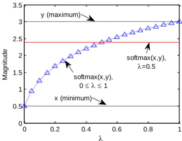
x
0
.
5
andy
3
as minimum and maximum values, respectively. Fig. 1 illustrates the effect of
on the result of soft-max operator. The result of soft-max for
0
.
5
is also shown in this figure. As can be seen, the result with5
.
0
which is equal to 2.386, tends themaximum. As can be seen, assuming
0
.
5
, the value of weighted soft-max operator is
2
.
386
, which tends the maximum valuey
.In addition, the result of weighted soft-max is dependent on the amount of
such that for1
5
.
0
, it is closer to the maximum while for5
.
0
0
, it tends more to the minimum. For extremes
0
and
1
, the results of soft-max are equal to the minimum and the maximum values, respectively.We further consider
x
andy
as two scalar variables having 21 values shown in Fig. 2. In this figure, from left to right,x
has twenty one increasing values from 0 to 6 whiley
has twenty one decreasing values from 6 to 0. The results of max operator are shown with an extra value of 0.2 to distinguish fromx
- andy
-points. The results of soft-max operator are also shown for
0
.
5
and
0
.
85
. As can be seen, the results with
0
.
5
tend the amounts of maximum ofx
andy
, especially in cases where the maximum is much bigger than the minimum. As opposed to the max operator, the result of soft-max, is affected from both maximum and minimum. The results of soft-max for
0
.
85
are closer tox
thanthose for
0
.
5
, eitherx
is minimum or maximum. On the other hand, choosing
0
.
5
, the effect ofy
on the soft-max result is increased. As a result, unlike max operator which its value is equal to the amount of maximum, the value of soft-max is a function of both maximum and minimum values.B. Weighting factors for the proposed algorithm
To further improve the performance of the adaptive algorithm, time-varying weighting factors
)
(
n
and1
(
n
)
are assigned tow
i(
n
)
and)
(
n
f
, respectively. Therefore, the weighted soft maximum is proposed instead of a maximum, as
(
)
exp
|
(
)
|
1
(
)
exp
(
)
log
)
(
n
f
n
n
w
n
n
i i
(14) for
i
0
,
1
,
...,
N
1
.As will be explained in the next section, to expedite the convergence of algorithm, the weighting factor
(
n
)
could be a decreasing function with time such that when the active coefficientsw
i(
n
)
reach tothe final values, all proportionality functions
i(
n
)
approach the amount of
f
(
n
)
.C. Experimental validation of the proposed
algorithm
To validate the steps of our proposed soft-max PNLMS (SM-PNLMS) algorithm, we conduct some simulation experiments. In the first experiment, we evaluate the performance of SM-PNLMS employing time-invariant
(
n
)
. Similar to [12], the input signal is assumed to be correlated unity-variance AR(2) as follows,)
(
)
2
(
)
1
(
)
(
n
b
1x
n
b
2x
n
u
n
x
(15)where
b
1
0
.
4
,b
2
0
.
4
, andu
(
n
)
is a white Gaussian noise with variance
u2
0
.
77
. InFigure 3: Validation of the proposed algorithm
0 500 1000 1500 2000
-40 -35 -30 -25 -20 -15 -10 -5 0
No. of iteration
M
is
a
lig
n
m
e
n
t
(d
B) =0.01
NLMS PNLMS
=0.5
=0.99
Figure 6: Variation of
(
n
)
with respect to the value of
0 500 1000 1500 2000
0 0.2 0.4 0.6 0.8 1
No. of iteration
V
a
lu
e
o
f
=0.1
=0.2 =1 =0.5
=0.25
addition,
0
.
5
and the measurement noisev
(
n
)
is white Gaussian with variance
v2
10
3 to achieve SNR=30 dB. The sparse impulse response is assumed with lengthN
100
and includes only four active coefficients at locations{
1
,
30
,
35
,
85
}
with values equal to{
0
.
1
,
1
.
0
,
0
.
5
,
0
.
1
}
.For evaluation, the normalized misalignment measure (in dB) is employed as [12]
2 2 10
||
||
||
)
(
||
log
20
)
(
o
o
n
n
w
w
w
. (16)The resulted normalized misalignment errors are averaged over 100 independent trials. Fig. 3 illustrates five misalignment curves which are derived from NLMS, standard PNLMS, and the proposed algorithm
with time-invariant weighting factors
99
.
0
,
5
.
0
,
01
.
0
. The performance of NLMSand PNLMS are shown for comparison. It is notable from Fig. 3 that employing weighting factor
99
.
0
results in the highest convergence rate with the maximum steady-state misalignment error. On the other hand, employing
0
.
01
results in a slow convergence, close to that of the NLMS. In addition, the performance of the proposed algorithm with
0
.
5
is close to that of PNLMS.D. Modified version of the proposed algorithm
As shown in Fig. 3, values of
(
n
)
close to one, results in a higher convergence rate while lower values of
(
n
)
cause the algorithm to achieve a less steady-state error. As a result, to expedite the convergence, one can reduce the weighting factor
(
n
)
gradually such that all the proportionality functions
i(
n
)
approach the scalar
f
(
n
)
. Asf
(
n
)
is the same for all coefficients, in such a case, the SM-PNLMS behave similar to the NLMS algorithm. As can be seen from Fig. 3, the NLMS algorithm achieves the minimum steady-state misalignment error. Therefore, we expect the SM-PNLMS algorithm achieves a low steady-state error, once the amount of
(
n
)
becomes low (near zero). In order to decrease the weightingfactor, we initially employ the following linear function:
)
1
(
)
(
n
n
(17)where
0
1
is a constant which should be close to one such as to decrease the weighting factor slowly in accordance with the convergence time. Fig. 4 illustrates the variation of misalignment for various amounts of
. A small
(still near one) means a fast transition of
(
n
)
from one to zero, while a bigger
very close to one means slow variation of
(
n
)
. The variations of
(
n
)
with respect to
are shown in Fig. 5.As can be seen from Fig. 4, for
0
.
99999
the algorithm acts similar to the case of time-invariant)
(
n
. The reason is because the variation (reduction) of
(
n
)
-as shown in Fig. 5- is so slow that we could assume that variation is negligible. On the other hand, for smaller
, for example
0
.
96
,
(
n
)
dramatically drop to zero and hence, convergence behavior of the algorithms are close to that of NLMS, as shown in Fig. 4.
Figure 4: Variation of misalignment with respect to the amount of
0 500 1000 1500 2000
-40 -35 -30 -25 -20 -15 -10 -5 0
No. of iteration
M
is
a
lig
n
m
e
n
t
(d
B)
=0.99999 NLMS
=0.999 =0.99 =0.98 =0.96
Figure 5: Variation of
(
n
)
with respect to the value of
0 500 1000 1500 2000
0 0.2 0.4 0.6 0.8 1
V
a
lu
e
o
f
No. of iteration
=0.96
=0.99
=0.98
=0.999 =0.99999 =0.9999
Figure 8: Variation of
(
n
)
in terms ofn
0 2000 4000 6000 8000 10000 12000 14000 0
0.2 0.4 0.6 0.8 1
No. of iteration
V
a
lu
e
o
f
Figure 7: Comparison of our proposed algorithm with other PNLMS algorithms
0 500 1000 1500 2000
-40 -35 -30 -25 -20 -15 -10 -5 0
M
is
a
lig
n
m
e
n
t
(d
B)
No. of iteration PNLMS
NLMS
SM-PNLMS
Figure 9: Comparison of our proposed algorithm with other PNLMS algorithms
0 2000 4000 6000 8000 10000 12000 -40
-35 -30 -25 -20 -15 -10 -5 0
No. of iteration
M
is
a
lig
n
m
e
n
t
(d
B)
NLMS PNLMS SM-PNLMS MPNLMS IPNLMS
E. Further modification: A weighting factor based on
an estimation of MSE
As mentioned in (17), the value of
(
n
)
and hence, the performance of algorithm strongly depends on the parameter
and the starting point
(
0
)
which is not desirable. In addition, as shown in Fig. 4, for
's close to one, typically
0
.
99999
, the steady-state misalignment of the proposed algorithm is relatively high in comparison to that of the NLMS and PNLMS algorithms. On the other hand, for a smaller
, typically 0.96 in our simulation
(
n
)
drop to zero very fast, before finalizing the convergence. As a result, the algorithm behaves similar to the NLMS algorithm, during the convergence and hence, its convergence rate is reduced. To mitigate this issue,
(
n
)
could be reduced gradually with convergence of the algorithm. To this end, we may correlate the weighting factor with the MSE of the adaptive filter. When the algorithm is in initial stages of convergence, the MSE is high and thus the value of
(
n
)
should be near one. After decreasing the MSE error floor, the amount of weighting factor should be decreased.We estimate the MSE by averaging the square error
)
(
2n
e
by a one pole low-pass filter as
0
),
(
)
1
(
)
1
(
0
),
(
)
(
2 2
n
n
e
n
n
n
e
n
(18)where
0
1
is the forgetting factor and typically is assumed to be close to one.We then make
(
n
)
to be a function of the estimated MSE, so that it could reduce gradually during the convergence of algorithm. To this end, we define
(
)
(
)
)
(
n
n
maxn
(19)as scaled and normalized output MSE, where
)
(
log
)
(
n
10
n
and
(
0
),
,
(
)
max
)
(
max
n
n
. The parameter
is a constant which can be chosen such that to be inversely proportional to the amount of the estimated steady-state MSE. According to the definition of (19),)
(
n
starts from zero and approaches
1
on the mean. Accordingly, we propose to assign
(
n
)
as
0
,
1
(
)
max
)
(
n
n
. (20)The summation
1
(
n
)
in (20) is to set the initial amount of
(
n
)
to be one. In addition, the max operation in (20) acts as a hard limitation to restrict the minimum amount of
(
n
)
to be zero. Therefore during convergence,
(
n
)
starts from one and gradually reduces to finally reach to a value near zero at the end of convergence.Fig. 6 illustrates the variation of
(
n
)
in terms ofn
for different values of
for the abovementioned simulation. The curves are obtained employing99
.
0
.Our extensive simulations illustrate that the performance of the proposed algorithm is not highly sensitive to the amount of
, however, a suitable choice to achieve a high performance is obtained when the amount of
is inversely proportional to the estimated steady-state MSE.Figure 10: The simulated acoustic room impulse response
0 50 100 150 200 250 300 350 -0.1 0 0.1 0.2 0.3 0.4 0.5 0.6 0.7 Sample index Am p lit u d e
Figure 11: Comparison of the proposed algorithm with other PNLMS based algorithms for a room impulse response.
0 1000 2000 3000 4000 5000 6000 7000 -25
-20 -15 -10 -5
No. of iteration
M is a lig n m e n t (d B ) SM-PNLMS IPNLMS MPNLMS PNLMS
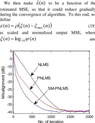
Now, if we replace the weighting factor (17) with the function of (20) and substitute (20) in (14), an improved performance for SM-PNLMS is obtained. A typical result using AR(2) input signal is shown in Fig. 7.
As can be seen, the convergence rate of SM-PNLMS is better than SM-PNLMS and NLMS so that misalignment of SM-PNLMS reaches -35 dB after 570 iterations while PNLMS and NLMS reach that level after 881and 1054 iterations, respectively. Table 1 illustrates the summary of the proposed algorithm. numerical simulations
In this section, we employ Monte Carlo simulations to evaluate the performance of the proposed algorithm and compare it with other
lgorithms. The results obtained by averaging over 10 independent trials. For all simulations, a colored speech-like signal is used as input signal. This signal is obtained by passing a white Gaussian noise through a
low-pass filter which has coefficients
0.3574]
0.9,
[0.3574,
[22]. Variance of input is assumed to be equal to
2x
1
. We evaluate ourproposed algorithm using
0
.
99
and
0
.
25
and compare it with NLMS, PNLMS, IPNLMS and MPNLMS.In the first simulation experiment, the sparse impulse response with length
N
256
is considered. The active coefficients are located at}
0,200,220
,50,100,12
1
{
with the values}
2,1.0
.5,0.4,-0.
0.1,1.0,-0
{
, respectively.The step-size is equal to 0.95 for all algorithms. The variation of
(
n
)
in terms ofn
is shown in Fig. 8. As can be seen, it gradually reduces from its initial value and after around 2000 iterations; it reaches below 0.2 which means the algorithm approaches NLMS after initial convergence. The variations of misalignment for algorithms are shown in Fig. 9. As we can see, to achieve
35
dB, the proposed SM-PNLMS algorithm requires 4000 iterations, while the MPNLMS, IPNLMS, PNLMS, and NLMS require about 5400, 5900, 8800, 14000 iterations, respectively. As a result, SM-PNLMS, achieves the fastest convergence rate among the mentioned algorithms.In the next simulation, we evaluate identification of a simulated acoustic room impulse response (RIR) which is derived using image methods [23]. For this simulation, the dimension of the room is
m m m
3
4
4
and the locations of the source and receiver are
1
,
0
.
95
,
1
.
5
meters and
1
.
1
,
1
.
05
,
1
.
53
meters, respectively. Fig. 10 shows the simulated RIR which is an example of sparse impulse responses.For simulation, the step-size is considered 1.2 for all algorithms and other specifications are same as the previous experiments. Fig. 11 compares the misalignment of the proposed SM-PNLMS algorithm ith its counterparts for the above RIR with length Table 1: The proposed algorithm
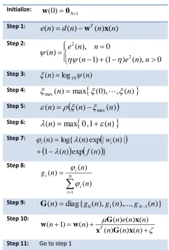
Initialize:
w
(
0
)
0
N1Step 1:
e
(
n
)
d
(
n
)
T(
n
)
(
n
)
x
w
Step 2:
0
),
(
)
1
(
)
1
(
0
),
(
)
(
2 2n
n
e
n
n
n
e
n
Step 3:
(
)
log
(
)
10
n
n
Step 4:
(
)
max
(
0
),
,
(
)
max
n
n
Step 5:
(
)
(
)
(
)
max
n
n
n
Step 6:
(
n
)
max
0
,
1
(
n
)
Step 7:
1 ( )
exp ( )
} | ) ( | exp ) ( log{ ) ( n f n n w n n i i
Step 8:
N i i i in
n
n
g
1)
(
)
(
)
(
Step 9:
(
)
diag
{
(
),
(
),...,
(
)}
1 1
0
n
g
n
g
n
g
n
NG
Step 10:
) ( ) ( ) ( ) ( ) ( ) ( ) ( ) 1 ( n n n n n e n n n T x G x x G w wStep 11: Go to step 1
333
N
. As can be seen, the proposed algorithm achieves a higher rate of convergence, so that its misalignment error reach
20
dB after 1400 iterations while it takes 1700, 2200, and 2800 iterations for IPNLMS, MPNLMS, and PNLMS, respectively.IV. CONCLUSIONS
We proposed a new Proportionate Normalized Least Mean Square (PNLMS) adaptive algorithm for sparse system identification. This algorithm employs a weighted soft maximum operator along with a variable weighting factor to achieve a high convergence rate. We experimentally found a formula for the weighting factor in terms of the estimated mean square error (MSE). Finally, we showed the superiority of our proposed algorithm over its counterparts using numerical Monte Carlo simulations.
ACKNOWLEDGMENT
H. Zayyani thanks Iran's National Elites Foundation. This work was supported in part by a grant from Iran's National Elites Foundation.
REFERENCES
[1] S. Haykin, Adaptive filter theory, 4rd ed.. Englewood Cliffs, NJ: Prentice Hall, 2002.
[2] S. F. Cotter and B.D. Rao, “Sparse channel estimation via matching pursuit with application to equalization,” IEEE. Trans. Communication, vol. 50, pp. 374–377, 2002. [3] S. Vedantam, C. Carbonelli, and U. Mitra, “Sparse channel
estimation with zero tap detection,” IEEE. Trans. Wireless. Communication, vol. 6, pp. 1743–1763, 2007.
[4] P. A. Naylor, J. Cui, and M. Brookes, “Adaptive algorithms for sparse echo cancelation,” Signal Processing, vol.86, pp. 1182–1192, 2006.
[5] J. Benesty, T. Gansler, D. R. Morgan, M. M. Sondhi, and S. L. Gay, Advances in network and acoustic echo cancelation, Berlin: Springer, 2001.
[6] R. K. Martin, W. A. Sethares, R. C. Williamson, and C.R. Johnson, “Exploiting sparsity in adaptive filters,” IEEE. Trans. Signal Processing, vol. 50, pp. 1883–1894, 2002. [7] G. Deng, “Partial update and sparse adaptive filters,” IET [8] Signal Processing, vol.1, pp. 9–17, 2007.
[9] R. L. Das and M. Chakraborty, “Sparse adaptive filters- an overview and some new results,” in: Proceeding ISCAS-2012, pp. 2745–2748, 2012.
[10] D. L. Duttweiler, “Proportionate normalized least-mean-squares adaptation in echo cancelers,” IEEE. Trans. Speech Audio Processing, vol. 8, pp. 508–518, 2000.
[11] J. Benesty and S. L. Gay, “An improved PNLMS algorithm,” in: Proceedings of the IEEE International Conference on Acoustic, Speech and Signal Processing, pp. 1881–1884, 2002.
[12] H. Deng and M. Doroslovacki, “Improving convergence of the PNLMS algorithm for sparse impulse response identification,” IEEE. Signal Processing Letters, vol. 12, pp. 181–184, 2005.
[13] F. de Souza, O. J. Tobias, R. Seara, and D. R. Morgan, “A PNLMS algorithm with individual activation factors,” IEEE. Trans. Signal Processing, vol. 58, pp. 2036–2047, 2010. [14] P. Loganathan, A. W. H. Khong, and P. A. Naylor, “A class
of sparsness-controlled algorithms for echo cancellation,” IEEE. Trans. Speech Audio Processing, vol. 17, pp. 1591– 1601, 2009.
[15] B. D.Rao and S. Bongyong, “Adaptive filtering algorithms for promoting sparsity,” in: Proceedings of the IEEE International Conference on Acoustic, Speech and Signal Processing, pp. 361–364, 2003.
[16] Y. Ju, J. Jin, and S. Mei “l_0 norm constraint LMS algorithm for sparse system identification,” IEEE. Signal Processing Letters, vol. 16, pp. 774–777, 2009.
[17] C. Paleologu, J. Benesty, and S. Siochina, “An improved proportionate NLMS algorithm based on l_0 norm,” in: Proceedings of the IEEE International Conference on Acoustic, Speech and Signal Processing , pp. 309–312, 2010. [18] R. L. Das and M. Chakraborty, “A zero attracting
proportionate normalized least mean square algorithm,” in: Signal Signal and Information Processing Association Annual Summit and Conference, pp. 1–4, 2012.
[19] J. Benesty, C. Paleologu, and S. Siochina, “Proportionate adaptive filters from a basis pursuit prespective,” IEEE. Signal Processing Letters, vol. 17, pp. 985–988, 2010. [20] F. Y. Wu and F. Tong, “Non-uniform norm constraint LMS
algorithm for sparse system identification,” IEEE. Communication Letters, vol. 17, pp. 385–388, 2013. [21] H. Zayyani, M. Babaie-zadeh, and C. Jutten, “Compressed
sensing block MAP-LMS adaptive filter for sparse channel estimation and a Bayesian Cramer Rao bound,” in: Proceeding MLSP2009, 2009.
[22] S. Boyd and L. Vandenbergh, Convex optimization, Camcridge University, 2004.
[23] M. Bekrani, A. W. H. Khong, and M. Lotfizad, “`A Linear Neural Network based Approach to Stereophonic Acoustic Echo Cancellation,” IEEE Trans. Speech Audio Processing, vol. 19, pp. 1743–1753, 2011.
[24] J. B. Allen and D. A. Berkley, “Image method for efficiently simulating small-room acoustics,” J. Acoust. Soc. Amer., vol. 65, no. 4, pp.943–950, 1979.
[25] J. Liu and S. L. Grant, "Proportionate Adaptive Filtering for Block-Sparse System Identification," IEEE/ACM Trans. Audio, Speech, Language Process., vol. 24, no. 4, pp. 623-630, 2016.
[26] R. L. Das and M. Chakraborty, "Improving the Performance of the PNLMS Algorithm Using l1 Norm Regularization," IEEE/ACM Trans. Audio, Speech, Language Process., vol. 24, no. 7, pp. 1280-1290, 2016.
[27] H. Deng and M. Doroslovacki, "Improving Convergence of the PNLMS Algorithm for Sparse Impulse Response Identification," IEEE. Signal Processing Letters, vol. 12, no. 3 pp. 181–184, 2005.
[28] S. Haykin, Adaptive Filter Theory, 5th Ed., Prentice Hall, 2013.
[29] B. Farhang-Boroujeny, Adaptive Filters, Theory and Applications, Wiley 1999.
Mehdi Bekrani received the B.Sc. degree from Ferdowsi University of Mashhad in 2002, and the M.Sc. and Ph.D. degrees from Tarbiat Modares University in 2004 and 2010, respectively, all in electrical engineering. From 2011 to 2013, he was a Research Fellow at Nanyang Technological University, Singapore. He is currently an assistant professor of electrical engineering at Qom University of Technology (QUT).
Hadi Zayyani received his B.Sc., M.Sc. and P.hD. degrees all in Electrical Engineering and all in the communications field from Sharif University of Technology in 2000, 2003 and 2010, respectively. From 2012 to now, he is assistant professor of Qom University of Technology (QUT).