THE EFFECTS OF MISSING TIME-VARYING COVARIATES IN MULTILEVEL MODELS
Sierra A. Bainter
A thesis submitted to the faculty of the University of North Carolina at Chapel Hill in partial fulfillment of the requirements for the degree of Master of Arts in the Department of
Psychology.
Chapel Hill 2013
ii
ABSTRACT
SIERRA A. BAINTER: The Effects of Missing Time-Varying Covariates in Multilevel Models
(Under the direction of Patrick Curran)
Multilevel models are commonly used in psychological research to examine
developmentally-motivated hypotheses concerning the within- and between- person effects of a time-varying covariate on some outcome. Whereas multilevel models are flexible to accommodate incomplete data on the outcome, missing time-varying covariates present significant challenges to researchers. Unless multiple imputation is used, missing time-varying covariates will lead to a loss of data. This project evaluated the effects of missing time-varying covariates and imputation of missing time-varying covariates in multilevel models using a multifaceted simulation study. My results showed that missing time-varying covariates can lead to biased parameter estimates. However this bias is likely minor
iii
TABLE OF CONTENTS
LIST OF TABLES...iv
LIST OF FIGURES...v
I. INTRODUCTION...1
II. METHOD...22
III. RESULTS...30
IV. DISCUSSION...41
iv
LIST OF TABLES Table
1. Table 1. Meta-model F-tests, Partial Values, and Average Parameter Estimates for Complete Data in Model 1 and Model 2………..49 2. Table 2. Model 1 Meta-model F-tests and Partial Values for
Each Simulation Factor in Missing Data Conditions………...50 3. Table 3. Average Parameter Estimates for Model 1 Missing
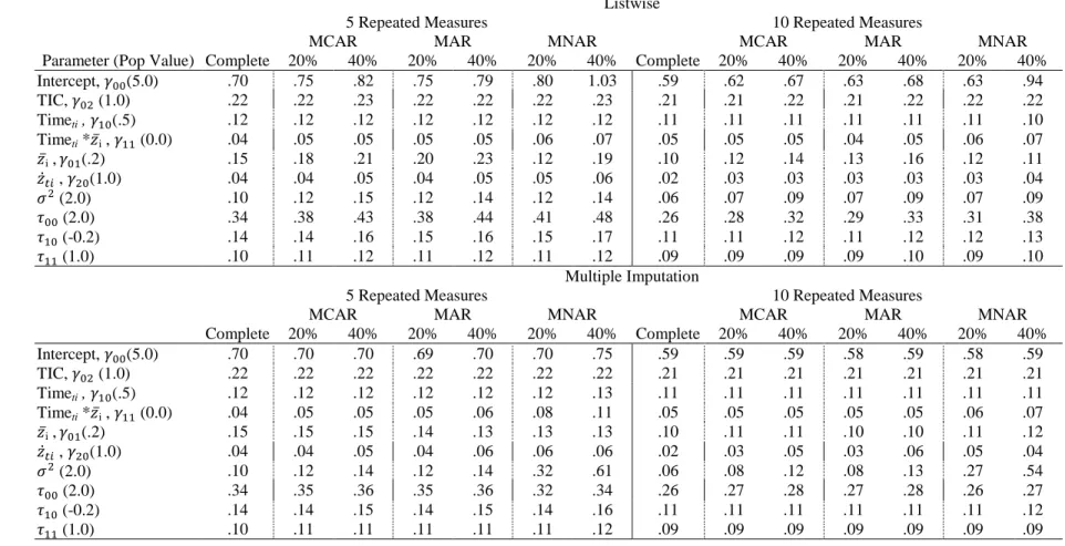
Data Conditions, 5 Repeated Measures……….………..51 4. Table 4. Average Parameter Estimates for Model 1 Missing
Data Conditions, 10 Repeated Measures………… ………..52
5. Table 5. Model 1 RMSE………..53
6. Table 6. Model 2 Meta-model F-tests and Partial Values for Each Simulation Factor in Missing Data Conditions………...54 7. Table 7. Average Parameter Estimates for Model 2 Missing
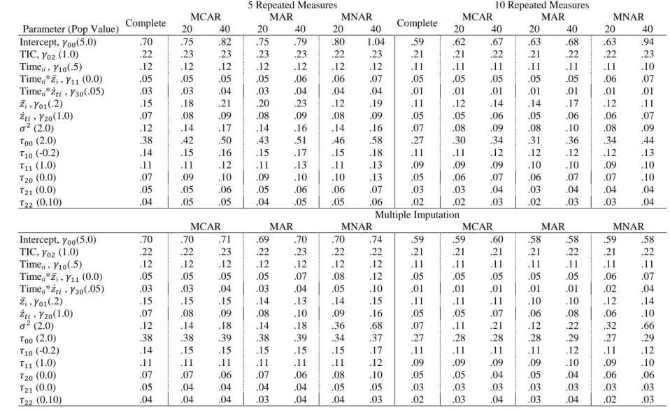
Data Conditions, 5 Repeated Measures………...55 8. Table 8. Average Parameter Estimates for Model 2 Missing
Data Conditions, 10 Repeated Measures………..……...56
v
LIST OF FIGURES Figure
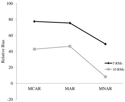
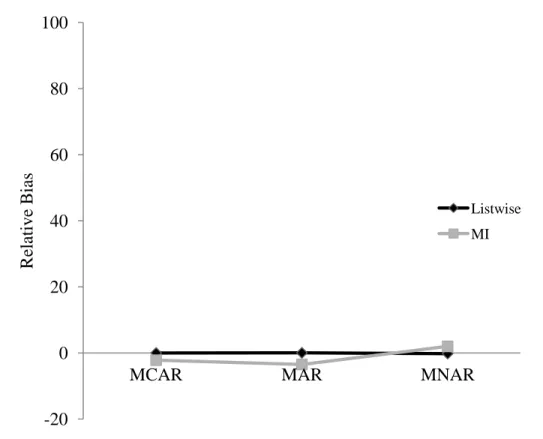
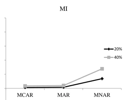
1. Figure 1. Effects of missingness mechanism and number of repeated measures on relative bias in the between-person effect ( ) in Model 1………58 2. Figure 2. Effects of mechanism and MI on relative bias in the within-
person effect ( ) in Model 1………..………...59
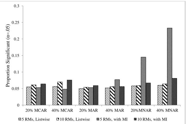
3. Figure 3. Effects of proportion missing and mechanism on relative bias in the residual variance estimate ( ) after MI in Model 1……….……….60 4. Figure 4. Proportion of significant estimates of the interaction
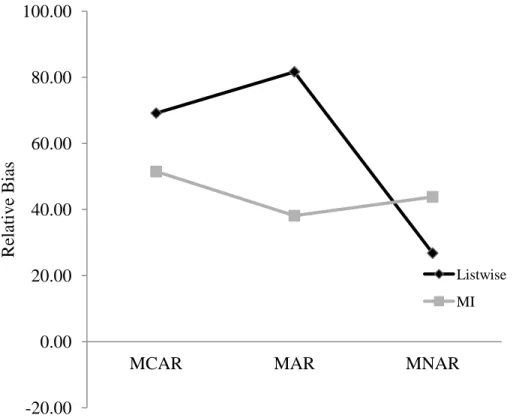
between time and the between-person effect ( ) in Model 1………...61 5. Figure 5. Effects of missingness mechanism and MI on relative bias
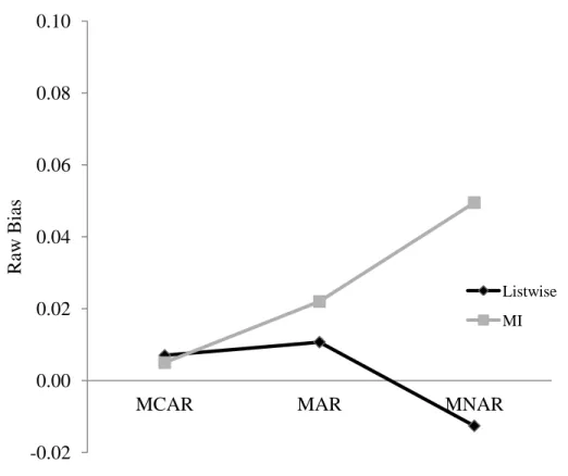
in the between-person effect ( ) in Model 2………...……….62 6. Figure 6. Effects of missingness mechanism and MI on raw bias in
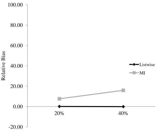
the interaction between time and the between-person effect ( ) in Model 2.……….………..63 7. Figure 7. Effects of percent missing and MI on relative bias in the
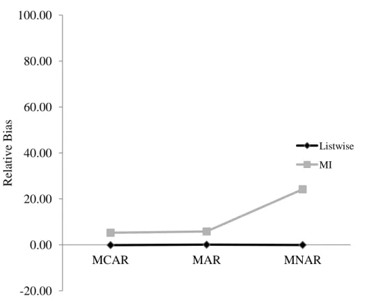
residual variance estimate ( ) in Model 2……….64 8. Figure 8. Effects of missingness mechanism and MI on relative bias
in the residual variance estimate ( ) in Model 2.………..65 9. Figure 9. Effects of missingness mechanism and MI on relative bias
in the interaction between time and the within-person effect ( ) in
CHAPTER 1
INTRODUCTION
Multilevel modeling (MLM) is a widespread technique for analyzing nested data. This flexible method can be used to study individuals nested within groups or repeated measures nested within individual. By modeling repeated measures nested within individuals, researchers can study important issues of inter- and intra- individual change over time
(Raudenbush & Bryk, 2002). Time-invariant covariates (TICs) such as gender and race can be incorporated to predict differences in these growth trajectories; in this way it becomes possible to address questions such as “Who developed an eating disorder?” and “Which
adolescents were at risk for drug use?”. Similarly, time-varying covariates (TVCs) can be incorporated to explore bivariate relationships between variables over time. TVCs predict time specific deviations from the underlying trajectory, answering questions such as “When
is disordered eating likely to occur?” and “When are adolescents engaging in drug use?” MLM fluidly extends to situations where the data are unbalanced or the outcome variable is incomplete for some participants (Raudenbush & Bryk, 2002, p.199-200).
Whereas a repeated measures ANOVA model requires all subjects to be measured at all time points, the MLM has no such requirement. Furthermore, MLM allows all participants to have different assessment schedules. The estimates of the MLM are chosen by maximum
2
outcome variable is incomplete, assuming the missingness is MAR (Enders, 2010, Chapter 4; Raudenbush & Bryk, 2002, p.199-200; Schafer & Graham, 2002). Another widely used missing data technique, multiple imputation (MI; Rubin, 1976), fills in the missing values with probable values while accounting for increased uncertainty in the parameter estimates. MI and ML perform similarly well when the outcome variable is incomplete, but MI is a more involved process (Allison, 2003; Olinsky, Chen, & Harlow, 2003; Schafer, 2003). Altogether, MLM requires a less rigid data structure than classical repeated measures ANOVA, and it also saves the analyst from the extra steps needed to multiply impute the incomplete data.
3
relationship with the outcome, predicting changes both in overall trajectory and in time specific deviations from this trajectory, and it is unclear what specific consequences missing TVCs could have on the estimation of these different effects in the model as well as the variance and covariance components.
Although this limitation of ML is known, the implications of listwise deletion of TVCs have received little attention. A thorough literature review and discussions with experts in missing data and multilevel modeling has revealed that the assumptions made on missing predictors in MLM and the potential consequences of this type of missingness have not been comprehensively studied or explained (however see Shin & Raudenbush 2007, 2010, 2011; and Liu, 2000 for recent exceptions).
The only way to combat listwise deletion in the current MLM framework is to use MI to impute the missing values before analyzing the data. MI is a useful and powerful method, but there are difficulties associated with MI, especially with longitudinal data, which I will describe later. Also, it has yet to be shown that MI will always lead to correct estimates no matter the population-level mechanism for TVC missingness.
In this research project I lay out the assumptions of missing predictors in multilevel models and empirically evaluate the consequences of list-wise deletion as a result of missing TVCs. For the purposes of this project I focus on the issue of missing TVCs, because this is unique to longitudinal data. I study a variety of population mechanisms for TVC
4
work to include useful model extensions that are useful to address developmentally-motivated research questions.
Traditional Multilevel Model
The traditional MLM with random slopes and intercepts is expressed as a set of level-1 and level-2 equations. The level-level-1 equation is given as
(1)
where is the outcome at time t for person i, and are the person-specific intercept
and slope respectively, and is the person and time specific residual. Time is commonly entered as wave of assessment or chronological age and scaled to the first measurement point so that measured waves 1-5 become timeti = 0-4. The values of time can be set as the
chronological age of each participant at assessment, grade in school, days of treatment, or any other time metric useful for the particular analysis question. Nonlinear growth can be modeled by introducing polynomial terms (i.e. include ).
The level-2 equations are
(2)
where and represent the population-average intercept and slope and and are the person specific deviations of the intercept and slope trajectory. The random slope and intercept growth model equation can be written in reduced-form as
(3)
5
actually estimated; rather the model estimates the (co)variance components of the random effects, so that VAR , VAR , and COV . The variance of the person and time specific residuals can be restricted to be constant over time VAR
or allowed to vary by time so that VAR .
One useful implication of the MLM structure is that the variance of is partitioned into between and within-person variance. The intra-class correlation (ICC) is the proportion of between-person variance, calculated from an unconditional model as:
(4)
where is the element of corresponding to the variance of . The statistic ranges from
0 to 1, and a high ICC indicates that repeated measures are highly correlated within individual, whereas a low ICC implies that the repeated measures within individual are weakly related. Later in this paper I will discuss an important implication the ICC has on between-person effect estimation.
TICs, person-level predictors such as gender or alcoholism diagnosis, predict between-person differences in the intercepts and slopes. Below a single TIC, denoted , enters the model at level 2. Notice the subscript to indicate a person-level effect.
(5)
Including TVCs is slightly more complicated; although technically time itself is a time-varying covariate because its value changes from one observation to the next. The effect of an additional TVC can be examined by adding it to the level-1 equation.
(6)
6
(7)
The random effect , allows the magnitude of the relation between the TVC and the outcome to vary across individuals. This random effect (or any other random effect) is optionally included. Note that TICs can be included in each of these level-2 equations to explain variability in the intercepts, slopes, or effect of the TVC.
The information captured by a TVC can describe both between- and within-person effects, and simply including the raw TVC at level 1 captures an un-interpretable aggregate effect (Kreft, de Leeuw, & Aiken, 1995; Raudenbush and Bryk, 2002, p. 183). This aggregate effect is weighted composition of the between- and within-person effects. Between-person effects are captured by the mean level of the TVC and within-person effects are the
corresponding deviations from this mean (Kreft, de Leeuw, & Aiken, 1995). There are two approaches to disaggregating these effects, and they differ by their approach to centering the TVC, which can either be centered with respect to the grand-mean or with respect to the person-mean (Kreft, de Leeuw, & Aiken, 1995; Raudenbush and Bryk, 2002, p. 183). The simplest method for interpretation is to person-mean center by including the person specific mean at level 2, denoted , and including the person-mean centered TVC, at level 1. The
set of equations becomes: Level 1:
(8)
Level 2:
7 Reduced-form:
(10) As Curran and Bauer (2011) point out, this approach to estimating TVC effects assumes that the TVC is unrelated to the passage of time. If there is growth in the TVC over time,
additional adjustments are needed to obtain correct between- and within-person effect estimates.
By person-mean centering in this way the between- and within-person effects of the TVC are untangled and can be examined separately. This is important because a TVC can exhibit (1) both a between-person effect and a within-person effect (operating in the same or opposite directions), (2) a between-person effect but no person effect, (3) a within-person effect but no between-within-person effect, or (4) neither type of effect (see Curran & Bauer, 2011 for a discussion on disaggregating effects).
The model can be extended even further to allow one or more TICs to predict differences in the effect of the TVC or by including interactions. For example, the effect of the TVC could differ for men and women, or it could differ depending on the overall level of the TVC, . The effect of the TVC can even interact with time, meaning the magnitude of the relation between the TVC and the outcome changes with time. These extensions are included below to create a final, general model.
Level 1:
(11)
Level 2:
8
Reduced-form:
+ )
(13)
This expanded model includes fixed effects for the overall-intercept ( ), between-person effect of the TVC ( ), between-person effect of the TIC ( ), overall-slope ( ),
effect of the overall level of the TVC on the slope ( ), effect of the TIC on the slope ( ),
overall within-person TVC effect ( , effect of the overall level of the TVC on the within-person TVC effect ( ), effect of the TIC on the within-person TVC effect ( ), overall TVC by time interaction ( ), effect of the overall level of the TVC on the TVC by time
interaction ( ), and effect of the TIC on the TVC by time interaction ( ). The random
effects for the intercept ( ), slope ( ), TVC ( ), and TVC by time interaction ( )
allow all of these effects to vary across individuals. Finally, the level-1 residual ( ) accounts for additional unexplained variability.
As with any statistical model, a number of assumptions underlies all of these models. I will detail these in the next section.
Model Assumptions
9
that the level-1 residual variance is equal at all time points is referred to as homoscedasticity and can be relaxed if needed at the cost of some parsimony. In longitudinal data analysis it is often necessary to relax the assumption of homoscedasticity; for example, it is common to observe that the residual variance increases with time.
At level 2, all q random effects are assumed to be conditionally independent across levels and multivariate normally distributed with mean equal to zero and covariance matrix , or: . The random effects and residuals are also assumed uncorrelated
across levels of the model, so that for all random effects q.
All predictors, whether level-1 or level-2, are assumed to be independent of and
. This means that and for all q random effects and
likewise and for all s predictors.
Furthermore, predictors are assumed fixed and known and thus without measurement error. This means that no assumption is made about the distribution of the predictors. Instead, distributions are assumed for and . Taken together, the above model structure implies a marginal distribution for and values for the means and (co)variance components of the observations within and between individuals, and all of these distributions are conditional on the fixed values of the predictors. The assumption that the predictors are treated as fixed and known in particular is a key focus in this project.
Bias in the Between-Person Effect
10
Marsh et al., 2007; Preacher et al., 2011; and Shin & Raudenbush, 2010). The problem is the traditional multilevel model does not account for measurement error in the predictors; instead predictors are treated as fixed and known. Estimating the person mean is necessary to
disaggregate between- and within-person effects, but there is error in this person mean just as error is expected in a sample mean. In other words, the person-specific mean is used as a predictor (fixed and known), but the person-specific variability around this mean is ignored. Ignoring this variability around the person-mean assumes that the mean is measured without error for all persons.
Sampling error in the person mean leads directly to bias in the between-person effect. The extent of this bias depends on the number of repeated measures, the ICC of the TVC, and the magnitude and direction of the between- and within-person effects. Lüdtke et al. (2008) gave a formula for the bias, assuming an equal number of repeated measures for all
individuals. Below we see that the expected difference between the estimated between-person effect ( ) and the true effect ( ) will be in the direction of the true within-person effect ( ):
(14) This formula also shows that a crucial element of this bias is the number of repeated measures, T. When the number of repeated measures is small, as is often the case in
11
Stawski, 2009). The extent of the bias can only be known in simulated data when the population parameters are known, but the direction of the within-person effect will indicate the direction of the bias.
So far I have only considered the implications of between-person effect bias if the data are completely observed and all individuals have the same number of repeated measures. If some measures of the TVC are missing, this will likely increase sampling error in the person mean. In all cases, if the between-person effect is biased, this bias will spread to related estimates in the model (Lüdtke et al., 2008). As I discussed previously, TVCs have the potential to be unobserved in a study, so the implications of missing TVCs should be better understood. In the next section I provide a brief overview of missing data theory.
Overview of Missing Data Theory
The foundation of missing data theory and the widely accepted taxonomy of missing data mechanisms was originally described by Rubin (1976). The key idea behind Rubin’s theory is that missingness is a variable with a probability distribution. Define a binary
variable R as a missing data indicator that takes on a value of 1 when a value is observed and 0 when missing. In the case of multivariate missingness the missingness indicator R becomes a matrix, R. The probability distribution of R is the probability of missing data, and this probability may or may not be related to other variables in the data. The hypothetical complete data is partitioned into observed and unobserved portions ( and ), and we want to understand the , where is a parameter or set of
12
are missing at random (MAR), missing completely at random (MCAR), and missing not at random (MNAR). I will briefly explain each in turn.
If the data are MAR then the probability of missingness on a variable Y is related to another variable (or variables) in the analysis but is unrelated to the missing values of Y. For example, if the probability of missingness is higher for minority groups, the assumption of MAR will be met as long as minority status is included in the analysis. Similarly,
missingness could relate to time such that individuals are less likely to be observed at later time points. In the case of MAR missingness, the probability of missingness reduces to:
(15) MCAR is a special case of MAR, and is the mildest form of missingness. If data is MCAR, this means the probability of missingness is unrelated to any values in the data, either observed or unobserved. The probability expression reduces to:
(16)
This assumption is the most stringent, and MCAR data are rare in practice. Important exceptions are planned missingness designs and completely arbitrary losses of data.
Finally, if data are MNAR, this means the probability of missingness depends on the missing values themselves, and the probability expression cannot be reduced.
(17)
13
when dealing with data assumed to be at least MAR (Schafer & Graham, 2002). To limit my focus, I will exclude techniques for handling MNAR data.
Listwise Deletion
Until recently researchers had little choice but to use a variety of outdated techniques for handling missing data, none of which are generally advisable. It is not my intention to comprehensively list or argue against these techniques here, but see Enders (2010) and Schafer and Graham (2002) for more details.
Of interest to this project is the practice of listwise deletion, also called complete-case analysis. Listwise deletion is often the easiest way to handle missing data by simply
excluding it from analysis. This reduces sample size and power and requires the restrictive missingness assumption of MCAR. Use of this outdated technique is unwarranted, especially given that more appropriate alternatives are available. Superior techniques like ML and MI do not require the unrealistic and unnecessarily strict assumption of MCAR and can avoid wastefully discarding data.
Maximum Likelihood
14
all the available data it will outperform listwise deletion even if data are MCAR (Enders, 2001).
The point of maximum likelihood estimation is to choose the population parameters that maximize the likelihood of observing a particular sample (for a straightforward overview of ML, see Enders, 2010, Chapters 3 & 4). This process begins by specifying a distribution for the population, and in the social sciences this is usually univariate or multivariate normal. In the multivariate case the distribution is expressed by a probability density function which describes the height of the curve for the vector of scores obtained for case i. For each
the value of gives the relative probability of observing a particular set of scores from a normally distributed population with the specified population mean vector and covariance matrix .
Assuming independent observations, the likelihood of the sample is the product of the likelihoods for each score, and the goal of maximum likelihood estimation is to maximize this likelihood by auditioning different values for and . In practice it is easier to maximize the log-likelihood to avoid rounding error and because the sample log-likelihood is the sum (rather than the product) of the individual log likelihood values.
Assuming a multivariate normal distribution for the data, the equation for the complete data individual log likelihood is:
(18)
The term gives the standardized distance between each score and the
15
ML estimation easily generalizes to accommodate incomplete data. The equation for the individual multivariate log likelihood for incomplete data is:
(19)
The only difference between the two equations is subscripting of the parameter matrices. These matrices are now allowed to conform to the dimensions needed to describe the complete data for each case.
Software programs choose starting values for the estimates and then use iterative optimization algorithms to adjust the estimates until “convergence” is reached. Convergence occurs when the change in log-likelihood from iteration to iteration becomes essentially zero; at this point the log-likelihood is maximized and the algorithm has arrived at the maximum likelihood estimates. ML estimation extended to incomplete data is virtually automatic to estimating the parameters in MLM software, and is therefore understandably the missing data procedure of choice for most researchers conducting MLM. Unfortunately, ML estimation is not without its limitations.
Limitations of Maximum Likelihood in Multilevel Models
There is an important instance when ML is inadequate. ML estimation is well-suited for situations where the outcome is missing, but when predictors are missing this estimation is not possible. To see why ML cannot proceed with missing predictors, look again at Equation (19) for the individual log likelihood when missing data is present. Implied by this equation is that a distribution is specified for the outcome variable, but nowhere is a
16
values of the predictors. It is useful to note that this is the meaning of the MLM assumption stated previously that the predictors are assumed fixed and known.
The above explanation is simple, but the severe consequence is any cases with
missing predictors in MLM are excluded from analysis (Enders, 2010, p. 276-278). Even if Y is present, it will be excluded as well, and this is analogous to the outdated practice of
listwise deletion of observations. This problem is not isolated to MLM; it is a fundamental feature of conditional likelihood. What is a unique issue to MLM is the presence of multiple levels of predictors. If a TIC (person-level covariate) is missing, that entire subject is
excluded from analysis. Missing TVCs will exclude the associated wave for each subject from analysis, and this introduces some interesting complexities.
Not only does this omit a wave of data, it also decreases the amount of data available to compute the person-mean of the TVC and systematically missing TVCs will
systematically bias the person mean estimate. Since the person-mean is prone to
measurement error (Lüdtke et al., 2008), even unsystematic TVC missingness (that is TVCs that are MCAR) will increase measurement errors, and this is a non-trivial consequence which has yet to be studied. Further, in the case of systematically missing TVCs, missing due to an MAR or MNAR mechanism, will systematically bias the person mean. Many factors besides mechanism (i.e. MAR versus MNAR) will systematically impact the mean in
17
it is not an appropriate method for handling missing data if predictors are incompletely observed.
Multiple Imputation
The other widely used state-of-the-art technique for handling missing data, MI was proposed by Rubin (1987). Like ML, MI assumes MAR missingness and multivariate normality. Whereas ML estimates the parameters directly from the available data, MI creates complete data sets by filling in the missing values with plausible values. This process is repeated over m replications, creating m complete data sets. Each data set is analyzed separately, and the estimates and standard errors are combined using simple rules given by Rubin (1987).
The imputation phase of multiple imputation cycles between two steps. In the first step, the incomplete data are predicted from the complete data using regression equations based on the estimated means and covariances. Each predicted score is augmented with a residual drawn from the appropriate normal distribution with variances equal to the residual variance from the regression. The second step depends on Bayesian methodology to generate different estimates for the regression coefficients and ultimately to arrive at m plausible alternative versions of the complete data.
18
MI of multilevel data is more complicated than with single-level data. If single-level imputation methods are applied to a multilevel dataset, the method assumes the error
variance for a variable is homogeneous across time points (Schafer, 2001). Multilevel imputation methods rely on a particular iterative algorithm called the Gibbs sampler (see Casella & George, 1992), and currently these methods are not available in commercial statistical packages. In some cases, an easy fix is to impute the data in wide format (one record per subject). If the dataset is in wide format, single-level imputation allows the error variance to be heterogeneous across time points (Fitzmaurice, Laird, & Ware, 2011, p. 543). This is only appropriate if the data are rigidly structured, meaning all subjects follow the same assessment schedule. If this is not the case, imputing the data in wide format induces additional missingness and single-level imputation procedures will not work properly. For this masters project I simulated data, so the complications of unstructured data did not arise.
Multiple Imputation Versus Maximum Likelihood
It is well established that when the same variables are used in the model and when sample size is large, ML and MI yield practically identical results (e.g., see Allison, 2003; Newman, 2003; Olinsky, Chen, & Harlow, 2003; Schafer, 2003). However, both methods handle missingness in distinctively different ways, and they each have their advantages. In many instances, ML is easier to implement because it is not necessary to go through all of the steps required in MI before doing an analysis. However there are instances where MI should be preferred. For example, as Enders and Gottschall (2011) point out, if the ultimate goal of an analysis is to compute a scale score for subsequent analysis steps, only multiple
19
of missing TVCS, MI can preserve the item-level TVCs necessary for computing the person mean.
Additionally, MI makes it is easier to include auxiliary variables, which are potential correlates of missingness or the incomplete variables that are not of direct theoretical interest (Collins, Schafer, & Kam, 2001). Including these auxiliary variables can be helpful for satisfying the MAR assumption. Procedures outlined to incorporate auxiliary variables into ML analyses are currently cumbersome and infrequently used (see Enders, 2010). This is not an advantage of MI per se but is more a feature of the statistical software currently in use. It is reasonable to expect software will catch up and counteract this imbalance.
Finally, in the case of missing predictors in MLM, MI clearly holds the advantage over ML. MI is equally useful for missing predictors and missing outcomes.
Other Alternatives
The approaches I have presented here represent the traditional multilevel model and the options available within this framework. Other less widely available alternatives exist. Recently, Shin and Raudenbush (2007, 2010, & 2011) have proposed alternative MLM approaches that allow the model to be estimated using the joint likelihood instead of the conditional likelihood as described previously. Using this approach, listwise deletion of TVCs is avoided. This development is quite recent and not currently programmed in any commercially available software.
Joint likelihood estimation is also potentially available for analyzing longitudinal data in the structural equation modeling (SEM) framework. However, when interested in
20
this project I limited my focus to answer this question in the traditional MLM context because (1) this approach is in wide use and (2) the issue remains that the impact of missing TVCs has not been appropriately studied.
Research Hypotheses
Based on prior work by Lüdtke et al. (2008) and pilot simulation work I expected that TVCs missing by any mechanism would increase sampling error in the person-mean, and this would cause bias that would propagate throughout the model estimates. This bias due to sampling error in the person-mean should impact estimates of the fixed effects for the intercept, slope, between-person effect, and possibly interaction effects. The elements of T
should be sensitive to this error as well. With more repeated measures, the effects of TVC missingness should be less extreme. When substantial bias is present, it is possible that spurious effects may be detected. The within-person effect of the TVC and person-level variance were expected to remain stable. The effects of sampling error in the person-mean on more complex interactions with , and TICs had not been previously examined, and I
did not have prior hypotheses about these effects. Some evidence from pilot simulations suggested that a spurious * interaction may result from increased sampling error in
the person-mean.
21
CHAPTER 2
METHOD
To evaluate the impact of missing TVCs in multilevel models I carried out a computer simulation study. I simulated data consistent with a longitudinal multilevel model,
systematically imposed missingness, and multiply imputed the missing data. In this design I varied the percentage missing, the missingness mechanism, and the number of repeated measures. All data generation and analyses were done in SAS.
Data Generation and Model Design
The simulated data were consistent with a longitudinal growth model with a TVC (e.g., Equation 10). The ICCs of the TVC and the outcome were set to .50 when computed from unconditional models, a sufficiently high ICC to be reflective of longitudinal data. For simplicity, the level-1 error structure was homoscedastic, but this does not limit the
generalizability of the findings.
Many simulation studies focus on an artificially simple model, but in the present study I constructed more realistically complex models. As I have shown before, a variety of exciting hypotheses can be explored with TVCs in multilevel models, and I chose to evaluate the impact of TVC missingness on these motivating examples in order to have more
23
Model 1. Model 1 included random intercept and random slope (time) effects, and the TVC (e.g., internalizing) exerted both within- and between-person effects on the outcome (e.g., alcohol use). A binary TIC (e.g., gender) also asserted an intercept effect (i.e., a main effect on the outcome).
The level-1 and level-2 equations for Model 1 are shown below.
Model 1:
Level 1:
(20)
Level 2:
(21)
These population values were chosen to be representative of effects found in real
applications. The intercept ( ) was set to 5.00 with a TIC intercept effect 1.00 which represents that females started one unit (or 20%) lower than males. The between- ( ) and within- ( ) person effects representing the effects of internalizing on alcohol use are in the
same direction, where 1.00 and 0.20. This general pattern of within- and
between-person effects (in the same direction with a larger within-person effect) is a pattern often seen in real data (e.g. Armeli et al., 2005; Hardy et al., 2011; Jahng et al., 2011). The slope of alcohol use increased at a moderate rate of one half unit per wave, 0.50. Note that in these equations a term for the overall level of the TVC interacting with time ( is included, but the population value for this parameter is zero.
24
generated where σ 2 = 2.0. Likewise the random effects were multivariate
normally distributed, or: . Within , the intercept variance ( ) was
2.00, slope variance (τ11) was 1.00, and the intercept and slope covariance ( ) was -0.20 (with associated correlation -0.10), reflecting the common pattern that, in general, those who start higher increase at a slightly slower rate.
Model 2. Model 2 included all of the effects in Model 1. Additionally, Model 2 included a random person effect for the TVC and an interaction between the within-person TVC effect and time. Applications with random within-within-person TVC effects are not typically tested, but interesting examples have been published. In one recent example, Stawski, Mogle, & Sliwinski (2011) included a random within-person daily stressor effect to test for individual differences in this effect. The level-1 and level-2 equations are shown below in Equations 22 and 23.
Model 2:
Level 1:
(22)
Level 2:
(23)
The interaction term = 0.05 included in Model 2 signifies that the magnitude of
the within-person TVC effect increased modestly with time; this effect is included because it is relevant to developmental processes. The variance for the random within-person effect ( ) was 0.10, and this random effect did not covary with the intercept or slope (i.e.,
25
Sample Size and Number of Repeated Measures
Because sample size is unrelated to between-person effect bias and was not expected to play an important role in the conditions I examined, I held sample size constant at N=250 per data set. This relatively large sample size is representative of a large-scale study and was also chosen to help avoid any potential convergence issues with MI. In pilot work, MI had more difficulty converging in smaller sample size conditions. However, these convergence issues are nontrivial, and with real data it is impossible to simply increase sample size as can be done with artificial data. The purpose of my thesis was not to investigate convergence issues in MI, but more research in this area is needed to comprehensively ensure that MI for TVC missingness is viable in smaller samples.
The number of repeated measures was varied at 5 and 10. This is an important factor to vary because the number of repeated measures directly impacts the amount of sampling error in the person mean and should impact the magnitude of bias caused by list-wise deletion of TVCs. Both of these conditions are representative of traditional multi-wave designs.
Proportion of Missingness
26
repeated measures and 20% missing MCAR, wave 1 was completely observed and waves 2-4 had 20% missing from each wave.
Missingness Mechanisms
Each condition started with the same complete simulated data sets. TVCs from each complete data set were deleted consistent with an MCAR, MAR, and MNAR missingness mechanism in turn. The forms of missingness imposed here are intermittent, meaning a participant can have any pattern of missing and observed waves after the first time point. This is in contrast to the less general case of dropout missingness, where a participant never re-enters the study after the first missing wave.
To impose MCAR missingness, I simulated a random normal value for each TVC and ranked this random variable into 10 groups by wave. I then deleted TVCs from each wave (starting at wave 2) that corresponded to the appropriate number of highest groups for each percent missing condition (i.e., deleted 4 highest groups for 40% missingness condition). MNAR and MAR missingness was related to the values of the TVCs themselves such that higher values of the TVC were deleted, based on either the current TVC value (MNAR) or previous TVC value (MAR). Specifically, for MNAR missingness, the highest 20 or 40% of TVC values were deleted, by sample and wave. For MAR missingness, TVCs were deleted based on the highest 20-40% of previously observed values.
Analysis
27
to the detection of spurious effects, so to detect this I included a time by interaction in the model statement even though this interaction did not exist in either population generating model. In practice non-positive definite solutions are not retained, therefore to maximize external validity, replications with non-positive definite solutions were discarded.
After evaluating the impact of TVC missingness, each simulated data set was
multiply imputed using SAS PROC MI. In order to preserve the nested mean and correlation structure, each data set was transposed from long format to wide format before imputation. As recommended for intermittent missingness, the MCMC method was used with 1000 burn-in iterations for each chaburn-in (Schaeffer, 1997). The burn-initial mean and covariance estimates were derived for a posterior mode from the EM algorithm, which was also allowed a maximum of 1000 iterations. Following the recommendations of Graham et al. (2007), I carried out 20 imputations per data set. In certain conditions with high MCAR missingness and repeated measures, the posterior covariance matrices for MCMC were singular, and these replications were discarded. Information about discarded replications is presented in the results section.
After MI, the data were transposed back into long format and analyzed as before using SAS PROC MIXED. To be conservative and to avoid comparing results based on different numbers of imputations, replications in which any of the 20 imputations yielded a non-positive definite solution were discarded, and I will present more information about discarded replications with my results. Finally I used SAS PROC MIANALYZE to combine the estimates and standard errors for each data set.
28
this is the observed Type I error rate. Raw bias is simply the true value ( ) subtracted from the corresponding estimate ( )
(24)
Relative (or percentage) bias is computed as
(25)
and is simply raw bias scaled as a percentage of the population parameter. For the parameters that equal zero in the population model, such as the interaction between time and the
between-person TVC effect, this statistic is not defined because it would involve dividing by zero. RMSE is computed as
(26)
and because it is in the same metric as the data, it can be interpreted as representative of the size of a “typical” error. RMSE is not strictly a measure of bias; rather it takes into account the variance of the errors and the mean error, so RMSE will not necessarily be zero when a parameter estimate is unbiased.
The factors of the simulation were examined for each parameter using analysis of variance (ANOVA) models with raw bias as the outcome, separately for Model 1 and Model 2. These meta-models were used to identify the most important factors in the simulation for explaining bias in each parameter. First, I analyzed the complete data separately for Model 1 and Model 2 using a one-factor ANOVA to test the effect of five versus 10 repeated
29
MI), number of repeated measures (5 vs 10), proportion of missingness (20 v 40%), and missingness mechanism (MCAR, MAR, MNAR).
Because ANOVA has high power to detect significant effects, I used partial values of each effect as an effect size measure to screen for meaningfully large effects. Partial is computed as
(27)
where and are the sums of squared deviations from the mean,
representing between-group and within-group variability respectively. Corresponding to a conventional medium effect size (Cohen, 1988), I examined significant effects that produced a partial value of at least .06. Finally, I followed up appropriate main effects and
CHAPTER 3
RESULTS
First, I will present results from the complete data conditions for each model to validate that the data generation was correct and to examine bias in complete data. In the complete data conditions, I examined partial values from the ANOVA meta-models to assess the impact of the number of repeated measures on raw bias in the parameter estimates. I show that this bias is consistent with what we would predict from Lüdtke et al. (2008). Descriptively, I also examined RMSE and the proportion of Type I errors for effects that were zero in the population generating models. Second, I will present results from the missing data conditions. Once again, I examined partial values from ANOVA meta-models to detect meaningful main effects and interactions among the simulation factors. To untangle the interaction effects, I examined relative bias because of its meaningful metric as well as RMSE.
Complete Data Conditions
31
Model 1. As expected, there was considerable bias in the complete data, especially for the intercept ( ) and between-person TVC effect ( ), as shown in Table 1. In the ANOVA meta-model, there were substantial main effects for the repeated measures factor on the intercept and between-person TVC effect. With more repeated measures, bias decreased. The intercept was underestimated by about 13% and 11% relative bias for 5 and 10 repeated measures, corresponding to sizable RMSE values of .66 and .55.
In terms of raw bias, the between-person TVC effect estimate was overestimated by .13 with 5 repeated measures and .07 with 10 repeated measures, exactly as predicted by Equation 14 given the population generating values. Bias in the between-person effect corresponded to large relative bias, 66% and 35% relative bias for the 5 and 10 repeated measures conditions, respectively. RMSE, reflecting variability and bias, for the between-person TVC effect was .13 for 5 repeated measures and .09 for 10 repeated measures.
Model 2. The pattern of complete data results were essentially the same in Model 2 as observed in Model 1. The meta-model confirmed sizable effects of the number of repeated measures on intercept and between-person effect estimates. In terms of relative bias, the intercept was underestimated by about 13% with five repeated measures, or 0.66 RMSE. With 10 repeated measures, the bias decreased to 11%, or .55 RMSE. Similarly, relative bias in the between-person effect decreased from .33 with 5 repeated measures to .27 with 10 repeated measures.
Missing Data Conditions
I will present results for the missing data conditions separately for each model,
32
interactions with partial eta-squared values of .06 or larger, corresponding to a medium effect size.
Model 1. Meta-model results for Model 1 are summarized in Table 2. Meta-model results indicated that there were nontrivial effects for the intercept ( ), between-person
TVC effect ( ), within-person TVC effect ( ), and residual variance ( ). There were no effects of any factor on intercept variance ( ), intercept/slope covariance ( ), slope variance ( ), TIC effect ( ), or time ( ).
I will describe the patterns of effects separately for each parameter. Average
estimates, empirical standard deviations of the estimates, and relative bias for each parameter in the missing data conditions for Model 1 are given in Table 3 and Table 4, for 5 and 10 repeated measures respectively. The final numbers of retained replications (i.e., positive definite solutions and non-singular covariance matrices for imputation) for each cell in the design are also given in Tables 3 and 4. In Model 1, replications were only discarded in the ten repeated measures, 40% MCAR condition; 353 replications were discarded in this condition due to singular posterior covariance matrices for MCMC, which may cause
imputed values of some variables to be fixed. RMSE for all Model 1 parameters are given in Table 5.
Intercept bias.For the intercept estimate ( ), there were main effects of the number
33
multiple imputation, from 0.75 to 0.70 RMSE. The main effect on relative bias for the
number of repeated measures was more pronounced than the effect of MI. However, the main effect of MI does show that MI helps counteract intercept bias due to missing TVCs under these simulation conditions. Besides the main effects of the number of repeated measures and use of MI, no other factors or interactions among factors meaningfully predicted bias in the intercept parameter.
Between-person effect bias. For the estimate of the between-person effect ( ), the
34
Within-person effect bias. There was an interaction between missingness mechanism
and MI for the within-person TVC effect ( ) as well as main effects of mechanism and proportion missing. The nature of interaction is shown in Figure 2. The within-person TVC effect was generally estimated without bias before MI in all missingness conditions, however after MI this parameter exhibited some bias and the direction of the bias depended on the type of missingness. In the 10 repeated measures, 40% missing conditions, this parameter was estimated with relative bias less than 1 for MCAR, MAR, and MNAR missingness. However, after MI, this parameter was underestimated with relative bias of -4% for MCAR missingness and -6% for MAR missingness, but overestimated with 26% relative bias when the missingness was MNAR. This pattern corresponds to RMSE 0.03-0.04 before MI and 0.04-0.06 after MI. Figure 2 shows that the magnitude of this bias is fairly small relative to the size of the effect. The main effect of the proportion missing revealed that, in general, bias was greater with a higher proportion of cases missing. This is clear, for example, in the 10 repeated measures condition, after MI, where relative bias is 2% at 20% missing and 5.5% at 40% missing. This comparison is between modest RMSE values of 0.03 and 0.06.
Residual variance bias. The estimated residual variance ( ) was substantially
35
MI of MNAR missingness was more pronounced at higher percent missing: relative bias jumped from less than 1% to 29% after MI in the 40% MNAR, 5 repeated measures condition. The RMSE for this parameter was 0.12 before MI for 20% MCAR, MAR, and MNAR missingness (5 repeated measures). After MI RMSE was essentially unchanged for MCAR and MAR missingness but rose to 0.32 for MNAR missingness.
Type I Errors. To detect potential spurious effects caused by TVC missingness, I
examined the proportion of significant effects detected for an interaction between time and the between-person TVC effect ( ). Because this effect was zero in the population, the proportion of significant effects should be close to the chosen level in a correctly specified model. Figure 4 shows the proportion of significant estimates, or Type I error rate, for this parameter across all conditions in Model 1, setting = .05. In general, the Type I error rate stayed close to the nominal level, though in a few cases the rate is elevated after imputation.
Most noticeably, with 5 repeated measures and MNAR missingness, the Type I error rate is much higher after imputation. With 20% and 40% MNAR missing TVCs the Type 1 error rate reached 18% and 26% respectively after MI in the 5 repeated measures.
Interestingly, the error rate was not inflated after MI in the 10 repeated measures conditions, staying at 7% and 8% for the 20 and 40% missing conditions, respectively.
Summary of Model 1 results. In sum, Model 1 results indicated that TVC
missingness can substantially bias several model estimates, even if the missingness is
36
Model 2. Table 6 contains F-tests and partial values corresponding to each factor and interaction in the meta-models for Model 2. Mean estimates, standard deviations of the estimates, and relative bias for each parameter in the missing data conditions for Model 2 are given in Table 7 and Table 8, for five and 10 repeated measures respectively along with the number of retained replications within each cell. RMSE for all Model 2 parameters are summarized in Table 9.
The small random effect unique to Model 2 led to more non-positive definite
solutions, especially with only five repeated measures. Before MI, the five repeated measures conditions lost an average of 43 replications, and after MI an average of 199 solutions were discarded. With 5 repeated measures, all discarded replications, before and after MI, were due to non-positive definite solutions. In the 10 repeated measures conditions, few
replications were discarded due to non-positive definite solutions. The overall average number of replications retained was 964, but nearly all replications lost were in the 40% MCAR condition after MI. As in Model 1, this condition led to a high number of singular posterior covariance matrices which precluded MI, and 398 replications were discarded for this reason.
Meta-model results indicated that in Model 2, as in Model 1, there were nontrivial effects for the intercept ( ), between-person TVC effect ( ), and residual variance ( ).
Effects were also found in Model 2 for the between ( ) and within ( ) person TVC effect
interactions with time. Within the level-2 covariance matrix T, there was only an effect on the variance of the random within-person effect ( ), and no effects on any of the other covariance parameters. There were no effects of any factor on the TIC ( ), time ( ), or
37
Intercept bias. Just as in Model 1, there were main effects of the number of repeated
measures and MI on bias in the intercept estimate such that bias for the intercept decreased with more repeated measures and with MI. Relative bias was -16% (0.82 RMSE) with 40% MCAR and 5 repeated measures before MI and -13% after (0.71 RMSE). Similarly with 10 repeated measures and 40% MCAR, relative bias was -13% before and -11% after MI, corresponding to 0.67 and 0.6 RMSE. Again, this suggests that MI decreases bias in the intercept estimate caused by missing TVCs.
Between-person effect bias. As in Model 1, main effects of mechanism and repeated
measures predicted bias in the between-person effect ( ); additionally, in Model 2 there
was an interaction between mechanism and MI. Again, bias decreased with more repeated measures. For example, in the MAR, 40% missing conditions (before MI) relative bias was 107% (0.23 RMSE) with 5 repeated measures, and with 10 repeated measures relative bias decreased to 73% (0.13 RMSE). As shown in Figure 5, MI decreased bias for MCAR and MAR but not MNAR missingness. One example of this can be seen in the 20% missing conditions with 10 repeated measures: relative bias decreases from 43.99 to 36.21 after MI with MCAR missingness and from 55.20 to 30.98 with MAR missingness, but in the MNAR condition the estimate is downwardly biased at -30.82 relative bias before MI and
overestimed after MI with 39.77 relative bias.
Figure 5 also shows that the effect of listwise deletion of TVCs on the between-effect estimate differed considerably by mechanism. Relative bias was greatest with MAR
38
values for this parameter varied from 0.11-0.23 without MI to 0.10-0.15 with MI; these values are sizable considering the parameter value for the effect was 0.20.
Random within-person effect bias. Unlike in Model 1, no factors predicted bias in
the within-person TVC effect ( ) in Model 2. However, the random effect variance for this
parameter ( ), unique to Model 2, exhibited a meaningfully large main effect of MI such that the variance was underestimated after MI. Before MI, for example in Model 2 with 20% of TVCs MCAR and 5 repeated measures, relative bias for this estimate was trivial, at 1%, however after MI relative bias was -17%.
Bias in the time by between-person effect interaction. In Model 2 there was an
interaction between mechanism and MI for raw bias in the estimate of the interaction of time with the between-person effect ( ), though this interaction also neared the medium effect-size threshold in the meta-model for Model 1. This parameter was zero in the population generating model and therefore relative bias is not defined for this estimate; however, in terms of raw bias, MI increased bias in the MNAR conditions. This can be seen in Figure 6 and in the mean estimates for the models with 5 repeated measures, where bias was minimal for all mechanisms, between -0.02 and 0.02 for all missingness conditions before MI but increased after MI, particularly for MNAR missingness. The raw bias increased to 0.06 and 0.10 for MNAR 20% and 40% missingness (5 repeated measures), which corresponded to RMSE values of 0.08 and 0.12.
Residual variance bias. The estimated residual variance was substantially affected by
39
increased from the 20% to 40% missing conditions in the imputation conditions, but remained stable at essentially zero without MI. The second interaction, between MI and mechanism, is presented in Figure 8. This interaction shows that bias was negligible for all mechanisms before MI, but after MI bias increased slightly for MCAR and MAR conditions and substantially for MNAR conditions. Measuring variability and bias, RMSE values for this estimate varied considerably among the many conditions and was about 0.15 and 0.09 before MI for 5 and 10 repeated measures conditions, respectively. After MI, RMSE hovered around 0.16 for 5 repeated measures MCAR and MAR conditions, ranged between 0.11-0.22 for 10 repeated measures MCAR and MAR conditions, and jumped to 0.68 and 0.66 in the severe 40% missing 5 and 10 repeated measure MNAR conditions.
Bias in the time by within-person effect interaction. Bias in the estimated interaction
between and time ( ) was explained by a main effect of mechanism and an interaction between mechanism and MI, plotted in Figure 9. Bias was negligible with and without MI for MCAR and MAR missingness conditions, but after MI the estimate was greatly
overestimated in the MNAR conditions. Relative bias jumped from 12% to 177% with 40% of TVCs MNAR and 5 repeated measures; this was linked with an increase in RMSE from 0.04 to 0.10.
Type I Error Rates. In Model 2, the type I error rate for the interaction of time and
40
For and , which were both zero in the population, the proportion of significant
effects stayed close to or below the nominal desired alpha level in all conditions. This is evidence that Type I error rates for these estimates were not impacted by TVC missingness.
Summary of Model 2 results. As in Model 1, results in Model 2 indicated that TVC
CHAPTER 4
DISCUSSION
I used a comprehensive simulation study to test my theoretically derived hypotheses concerning the effects of missing time-varying covariates in multilevel models. To my knowledge, this is the first study to specifically examine the effects of missing TVCs. The results of my project provided support for my research hypotheses and also revealed many complexities related to this type of missingness.
My results demonstrate that listwise deletion of missing TVCs can clearly bias model estimates; these effects should be understood and taken into consideration by researchers. Although TVC missingness is not ideal, the results of my project also highlight that the effects of TVC missingness may be overshadowed by bias already present even in complete data due to person-mean sampling error. My study illustrates that most bias due to TVC missingness occurs by increasing sampling error of the person mean. More repeated measures protected against this bias in complete and incomplete data. The mechanism of missingness was important because it directly determines if MI is appropriate and also because it systematically biased the person-mean estimate. In many cases MI counteracted bias due to missing TVCs, with some exceptions, particularly when TVCs were MNAR. I will briefly describe the effects of each factor in my simulation study.
Effects of Repeated Measures
42
complete data. This result is consistent with what Lüdtke et al. (2008) predicted. When TVCs were missing, by any mechanism and in every condition in each model, bias was worse with five repeated measures than with 10. More repeated measures decreased bias in both the between-person effect estimate and the intercept estimate. For example, with 40% of TVCs MCAR and listwise deletion, relative bias in the between-person effect decreased from 97.71 with five waves of data to 55.49 with 10. It is apparent that bias in the between-person effect causes corresponding bias in the intercept. This is because the overall intercept estimate is forced downward to compensate for the overestimated between-person effect. With more repeated measures, a better estimate of the person mean is obtained, and the intercept estimate has less error for which to compensate.
These results can be generalized from the chosen set of population parameters to other population generating models. As shown in Equation 14, bias in the between-person effect will be in the direction of the true within-person effect. The intercept estimate will therefore be forced downward to accommodate upwardly biased between-person effects and vice versa, and the extent of the bias will of course depend on the magnitude of difference between the two effects, the ICC of the TVC, and the number of repeated measures.
43
first time point is always observed). With 10 repeated measures, cases with only one
observation are much less likely, and it is possible the increased Type 1 error rate is related to imputation of this extreme, imbalanced missingness in the five repeated measures conditions.
Effects of Proportion Missing
I hypothesized that more missing TVCs would create more bias. There was some support for this hypothesis in the main effects of proportion missing found for the residual variance estimate and the within-person effect. Overall, however, the proportion missing was not a powerful explanatory factor in these simulations. The effect of proportion missing on the residual variance estimate was related to mechanism and MI in Model 1 and MI in Model 2. My results showed that bias in the residual variance estimate increased with the proportion missing after imputation in Model 2. This increase also occurred in Model 1, but only after imputation of MNAR missingness.
I did find that more missingness led to increased bias in the within-person effect, but only in Model 1. Because the within-person effect was generally estimated with high
precision, bias due to increased missingness was noteworthy, but the magnitude of the bias was still small relative to the size of the effect, which had a population value of 1.00. For example in the 10 repeated measures, 40% missing conditions, the RMSE for this parameter was 0.03-0.04 before MI and 0.04-0.06 after MI. Surprisingly, increased missingness did not generally exaggerate bias in the between-person effect. This was likely due to the
complicated patterns of more prominent effects due to other factors such as missingness mechanism and the use of multiple imputation.
44
The mechanism of missingness was a key explanatory factor and was related to bias in several effects. As predicted, I found that the effect of mechanism frequently interacted with MI. Two major considerations are important in understanding these patterns of effects. First, MI is appropriate to correct for MCAR and MAR but not MNAR missingness.
Secondly, the mechanism of TVC missingness differentially impacted the person mean estimate.
In some cases MI counteracted bias, but there were also some important exceptions. The use of MI offset bias due to missing TVCs in the intercept effect estimate, but after imputation the bias returned to the extremely high levels exhibited in complete data. Surprisingly, MI did not decrease bias in the between-person effect overall.
When missingness was MNAR, MI produced bias in the between- and within-person effects and interactions with these effects and time, as well as in the residual variance
estimate. MI of MNAR missing TVCs also caused an increased Type I error rate of the interaction between the between-person effect and time. Statistical theory explains these effects, as it has been clearly established that MI is beneficial if missingness is at least MAR (Rubin, 1987). Unfortunately, if missingness is MNAR, we risk introducing bias by using MI. MI is not robust to the assumption of MAR missingness, though in applied research we must almost always depend on this assumption (see Enders, 2010; Schafer & Graham, 2002).
45
MI yields appropriate estimates for MAR and MCAR missingness (Rubin, 1987). Likely this finding is attributable to the considerable and widespread consequences of ignoring error in the person mean estimate. I believe the upwardly biased between-person effect may have obscured the more modest variance of the random within-person effect. This finding is especially interesting because it is not expected from missing data theory.
In sum, my simulation study clarified a number of key issues related to TVC
missingness. The potential effects of TVC missingness should be considered accounting for the extent of bias that could be present in complete data due to sampling error in the person-mean, especially if few repeated measures are available. Multiple imputation of missing TVCs relies on the usual assumption of MAR missingness. Finally, due to the extensive effects of ignored bias in the between-person effect, multiple imputation may obscure some subtle but important estimates, such as the variance of the random within-person effect.
Implications and Recommendations for Applied Research
46
limitations for modeling between- and within-person TVC effects. A promising alternative is latent growth curve modeling (LCM) in the SEM framework which can allow for
measurement error in the person mean to be accounted for (Curran et al., in press; Lüdtke et al., 2008). Based on the findings of this study, I propose three recommendations for applied researchers.
First, if a key research question concerns the between-person effect of a TVC, it should be a critical priority to decrease sampling error of the person-mean estimate. One way to do this is to collect more repeated assessments, but this option is rarely realistic. Instead, more reliable estimates of the TVC at each assessment may improve person-mean reliability; see Shrout and Lane (2012) for an excellent chapter on reliability. Equation 14 from Lüdtke et al. (2008) can be used to estimate bias in the between-person effect, which is also
informative of bias in the intercept estimate.
Second, I recommend researchers use LCM instead of MLM to model bivariate relationships between a TVC and outcome. The key remaining advantage of MLM over LCM is flexibility to accommodate three-level nested data structures (Curran, 2003), and in the case of higher level nesting LCM may be intractable for this problem, despite potential bias in the between-person effect. Otherwise, I see no reason why researchers should not use the LCM framework in order to obtain an unbiased estimate of the between-person effect. See work by Curran et al. (in press) for details on disaggregating between- and within-person TVC effects in LCM.
47
mean decreases, holding other factors constant, the effects of missing TVCs will decrease. In the LCM framework, either multiple imputation or joint maximum likelihood estimation will prevent listwise deletion of TVCs. Both procedures assume an MAR missingness
mechanism.
Limitations and Future Directions
The results from any simulation study can never be generalized to all cases. Parameter values were not varied in my simulation, but the majority of the findings would differ predictably given alternate sets of population parameters. Theoretically, TVCs could be missing an infinite number of ways, and there is no way to systematically study them all. Different forms of missing TVCs that do not systematically bias the mean would clearly not have the same effects on that estimate, however many of my results concerning missingness mechanism are generalizable. In this demonstration, the form of missingness was very strong and will almost certainly not be as strong in real data, though the extreme case presented here is still illustrative of the issue. The technique of MI I used may not be feasible for many researchers with less structured data. I do not believe this impairs the external validity of my results pertaining to MI, but a significant problem still remains to enable applied researchers to perform multilevel imputation using widely available software.
My study was limited to the standard multilevel modeling framework and did not consider strategies available in LCM. Another promising tool available in SEM is joint maximum likelihood estimation. With joint maximum likelihood, listwise deletion due to missing TVCs and the considerable complications of MI could be avoided. This has not been well-studied, but a future direction would be to compare joint maximum likelihood to
48
Conclusion
Missing TVCs are not ideal and listwise-deletion of missing TVCs may cause bias, but in many cases bias due to missing TVCs will be trivial compared to the bias that already exists in complete data due to error in the person mean. Potential bias due to missing TVCs will be less extreme with more repeated measures or if sampling error in the person-mean is otherwise reduced. MI can prevent loss of data but assumes MAR missingness at minimum. Missingness mechanism is impossible to determine in real data, and even if MNAR
missingness is suspected, no general strategy exists to appropriately correct for MNAR missingness.
Currently, many researchers are estimating between- and within-person TVC effects in MLM, and my results suggest that there is a strong likelihood this often impedes our ability to draw accurate inferences. The more important issue highlighted in this project is that the multilevel modeling framework has serious limitations for modeling bivariate
relationships over time. Alternative strategies for modeling these developmentally motivated relations are warranted. The SEM framework, because it is able to better address