Spatial methods in areal administrative data analysis

Introduction

Health care claims or administrative data often arise as electronic copies of paid bills generated from insurance companies, including the Medicare and Medicaid programs. Widely used by researchers, partially de-identified versions of these data are available from the Centers for Medicare and Medicaid Services (CMS), from states in the form of hospital discharge summaries, and from some private insurance companies. In order to protect patient’s privacy, the data are stripped of names and street addresses. In many cases, however, zip or county code is retained to facilitate studying geographic aspects of health care. One of the most widely known applications of geography to claims data is the Dartmouth Atlas of Health Care (www.dartmouthatlas.org). First released in 1996, this atlas maps services and some utilization patterns, grouping patients into hospital service areas and hospital referral regions using a rule that assigns each zip code to the facility that serves the plurality of residents of that zip code (though the service areas are subsequently “adjusted” to make the geography more continuous).

In practice, such de-identified administrative data need to be analyzed as areal(lattice) data [1]. That is, the data are available for analysis only as

de-identified summaries over geographical regions, such as counties or zip codes. There are two general strategies commonly used by health services researchers to incorporate geography into studies based on such data: using existing geopolitical units without grouping (zip, county, state, MSA, etc.), and combining existing geopolitical units using an ad hoc rule (e.g., the Dartmouth atlas). The former approach works quite well when studies focus on units with large numbers of beneficiaries (entire states or urban areas, for example) but faces problems with unstable estimates when applied to rural areas or for conditions that are relatively uncommon. Ad hoc combination of units may encounter difficulties because groupings might not accurately reflect underlying population distributions and may not maximize available information, particularly if the aggregation obscures small-scale spatial variation in the data. Even at finer scales, areal administrative data analysis runs the risk of ecological fallacy [2] and the modifiable areal unit problem (see e.g. Gotway and Young, for a review) [3].

An alternate approach is to use methods from

spatial statistics to smooth geographic patterns. This approach recognizes what geographers refer to as the “first law of geography” [4], which is that

Spatial methods in areal administrative data analysis

Haijun Ma, Beth A. Virnig, Bradley P. Carlin

School of Public Health, University of Minnesota, Minneapolis, Minnesota, U.S.A.

Correspondence to: Bradley P. Carlin, MMC 303, School of Public Health, University of Minnesota, Minneapolis, Minnesota 55455-0392, U.S.A. Email: [email protected]

Abstract

Administrative data often arise as electronic copies of paid bills generated from insurance companies includ-ing the Medicare and Medicaid programs. Such data are widely seen and analyzed in the public health area, as in investigations of cancer control, health service accessibility, and spatial epidemiology. In areas like political science and education, administrative data are also important. Administrative data are sometimes more readily available as summaries over each administrative unit (county, zip code, etc.) in a particular set determined by geopolitical boundaries, or what statisticians refer to as areal data. However, the spatial dependence often present in administrative data is often ignored by health services researchers. This can lead to problems in estimating the true underlying spatial surface, including inefficient use of data and biased conclusions. In this article, we review hierarchical statistical modeling and boundary analysis (wombling) methods for areal-level spatial data that can be easily carried out using freely available statisti-cal computing packages. We also propose a new edge-domain method designed to detect geographistatisti-cal boundaries corresponding to abrupt changes in the areal-level surface. We illustrate our methods using county-level breast cancer late detection data from the state of Minnesota.

data arising from neighboring units are often more highly correlated than non-neighboring units.When present,this underlying spatial structure needs to be accounted for in order to obtain valid inferences. Often, the spatial structure itself is of scientific interest, as when estimating an underlying geographic health care usage or risk surface.

While other thematic mapping approaches are possible, the most common output of an areal data analysis is a choropleth (shaded, using color or grayscale) map indicating the rough magnitudes of a particular variable for each unit (see e.g. Figures 1(a) and (c) below). Such maps are crucial for identifying which units are aberrant (large or small), as well as assessing overall spatial patterns in the map which may arise due to underlying spatially associated covariates. Recent developments in geographic information systems (GIS) technology has made the drawing of such maps (complete with physical features such as roads, railroads, streams, lakes, etc.) fairly easy for applied scientists in forestry, public health, urban planning, and so on. However, proper attention must still be paid to key cartographic issues such as the proper selection of map type, scale, data classification, and color schemes; see Dent [5] for a full discussion.

Although raw data maps and crosstabulations are important tools for summarizing administrative data, inherent randomness and bias can cause raw data summaries to be misleading. For example, the raw incidence rate, calculated as the ratio of observed disease cases versus population size at risk, is often of interest to health services researchers. However, a few unusual cases observed by chance over an area of small population can lead to an exceptionally high raw rate, misleading and insufficiently reliable for reporting. Modern statistical methods enable the user to both smooth and attach inferential

statements to choropleth maps, such as a determination of whether an apparent “hot spot” on a map is in fact statistically significant, or merely the result of an unlucky year in a thinly populated region. In particular, Manton et al. [6] developed random effects methods for obtaining smoothed county-level rates via empirical Bayes statistical methods. The U.S. mortality atlas of Pickle et al. [7] was influential in its use and discussion of these and other, less formal alternatives, such as headbanging (median smoothing; see e.g. Mungiole) [8]. Most recently, fully Bayesian hierarchical modeling methods permit complete flexibility in how the estimates borrow strength across similar (say, geographically adjacent) counties, hence result in improved estimation, prediction and mapping of underlying model features driving the data.

While areal estimation and smoothing remain of primary importance in administrative data analysis, the identification of statistically significant boundariesover a geographic surface is an increasingly important topic. This area is often referred to as boundary analysis or, less descriptively but more colorfully, wombling, a name that pays homage to an important early paper in the area [9]. Recently, there has been increasing interest among a wide range of researchers in the spatial problem of detecting barriers separating regions of high and low response for certain variables of interest. In the field of public health, wombling is useful for detecting regions of significantly different disease mortality or (in the case of administrative data) availability of care, thus improving decision making regarding disease prevention and control, allocation of society resources, and so on.

Our Bayesian modeling approach is flexible and allows consideration of models too difficult to

handle using traditional, “frequentist” statistical approaches. Bayesian analytic philosophy is also easy to understand and concordant with the accumulation of scientific evidence. A drawback of Bayesian modeling, however, is that the methods can be computationally intensive. Fortunately, the rapid development of appropriate computer hardware and software has spurred a corresponding growth in Bayesian methodology. Bayesian models are now broadly used and have become an accepted part of statistical practice in many areas; for example, roughly 10% of applications to the FDA Center for Devices and Radiological Health (CDRH) are now Bayesian.

A Bayesian model for the observed data y=(y1,...,yn) begins with a probability distribution

f(y| θ) called the likelihood, where θis a vector of unknown parameters. In turn,θis assigned a prior

distribution p(θ|η), where η is a vector of

hyperparameters. The prior distribution summarizes our (possibly quite vague) knowledge about θbefore we have seen the data y. If ηis not known, a fully Bayesian approach would specify a

hyperprior distribution for η. Alternatively, we might instead obtain an estimate ηˆ and use it as if

ηwere known; this “shortcut” is usually called an

empirical Bayes approach. Assuming for the moment that ηis known, inference concerning θ is based on the posterior distribution of θ, computable using ordinary probability calculus as

We refer to this formula as Bayes’ Theorem.The denominator is called the marginal distribution of the data y, which is free of θ. It is a scaling constant for the posterior distribution of θ and thus does not impact the distribution’s shape. Thus equation (1) is often expressed compactly as

Sadly, even when the likelihood f(y|θ) and the prior p(θ) have convenient, closed-form expressions, the posterior p(θ|y) may not. Indeed, equation (2) usually involves high-dimensional integration and has no analytical solution. Traditional numerical integration methods are often unstable or infeasible when θ is of high dimension. Fortunately, Markov chain Monte Carlo (MCMC) methods offer an iterative computational method suitable for solving this problem. In a

nutshell, MCMC methods sample values

θ(g)_{,g=1,...,G, from a convergent Markov chain}

whose stationary distribution is the posterior, p(θ|y).After convergence, empirical summaries of the θ(g)_{values may be used in statistical estimates}

and tests concerning θ. A variety of MCMC methods have been proposed, the most prevalent of which is the Gibbs sampler [10,11]. Once fit, Bayesian models may be assessed via residual analysis, and compared via penalized likelihood criteria such as the AIC [12], BIC [13] and, for hierarchical models, the Deviance Information Criterion (DIC) [14].

Regarding user-friendly software, WinBUGS is a computing package that carries out Bayesian analysis using MCMC techniques. It is freely available from the website www.mrc-bsu.cam.ac.uk/bugs. WinBUGS includes an easy-to-follow manual and several worked examples, and an online Flash tutorial is available at www.statslab.cam.ac.uk/~krice/winbugsthemovie .html. In addition to posterior summaries and areal maps, the DIC model comparison statistic can be automatically calculated within WinBUGS.As such, we use this package for all of the models mentioned in this article.

There is a large and growing literature on Bayesian analysis and MCMC methods. For further reading, see the textbooks by Carlin and Louis [11] or Gelman et al. [15]. Gilks et al. [16] offer an excellent summary of advanced MCMC methods for Bayesian analysis.

The remainder of this paper is organized as follows. Section 2 introduces terminologies and concepts of statistical areal rate estimation and boundary analysis, and gives a brief description of the dataset we use in this paper.Section 3 illustrates spatial smoothing hierarchical models using administrative data sets specific to cancer. This section also describes boundary analysis methods, including some that operate on the scale of the

edges between areas, as well as more traditional approaches that work with the areas themselves. Finally, Section 4 summarizes and discusses directions for future research in this area.

Geographic data in cancer rate estimation and boundary analysis

We illustrate our spatial hierarchical modeling methods using county-level data on breast cancer late detection in the US state of Minnesota.These data are aggregated over the years 1993 to 1997, and were collected by the Minnesota Cancer Surveillance System (MCSS), a population-based cancer registry maintained by the Minnesota Department of Health.We choose the county level partly for ease of illustration, but hasten to add that some smaller, sub-county unit (say, census tract) may well be more appropriate here; see e.g. Boscoe and Pickle [17 ]for a discussion of this issue in the context of public health data. p(y,θ) f(y|θ)p(θ)

p(θ|y) =

p(y) = ∫f(y|θ)p(θ)dθ

p(θ|y)∝f(y|θ)p(θ).

(1)

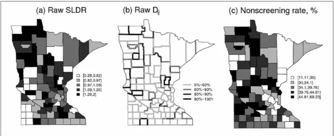
Maps of standardized late detection ratios (SLDRs) for the Minnesota breast cancer data are given in Figure 1(a). The SLDR for county i is calculated by dividing the observed value by the age-adjusted expected counts:

Here, the populations at risk Nk

i are the numbers

of incident breast cancer cases for age group kin county i, and the Yk

i are those detected late

(regional or distant stage); for more details see Thomas and Carlin [18]. The above approach to calculating the Eiis called internal standardization;

the counts can also be standardized externallyif an appropriate standard table of age-specific breast cancer detection rates is available.An SLDR less than 1.0 indicates fewer than expected breast cancer late detections in that county, while a value greater than 1.0 indicates more deaths than expected.The SLDRs in Figure 1(a) suggest a modest amount of spatial clustering in the data.

As mentioned above, in the analysis of geographic administrative data, interest focuses not only on estimation of area-level rates, but also on finding boundaries corresponding to significant changes in the underlying risk surface, a problem known as boundary analysis or

wombling. BoundarySeer is a commercial GIS-based boundary analysis software package; Figure 1(b) shows its application to our breast cancer late detection data. For areal data like ours, BoundarySeer uses the top k% of the boundary likelihood values, commonly defined as the absolute regional differences,

to determine the segments that comprise the boundary. In the figure, the darkest lines show the top 10% of the Dij ; note that these segments are

often disconnected. In addition, it is hard to know how much confidence to place in these boundaries, since the procedure has not accounted for the greatly varying sample sizes across the counties. For example, the Twin Cities metro area (on the east side of the state about one third of the way up) seems to include no more boundaries than any other region. Finally, the selection of k=10% seems quite arbitrary; the software will identify “boundaries” regardless of whether differences across regions are significant or not.

In the literature, there is debate over the effectiveness of mammography in reducing breast cancer late detection rates. Some studies have shown that mammography screening can reduce breast cancer mortality by 30-40% among women

aged 50 years and older [19,20]. A recent study of the National Cancer Institute also indicates that not having had a screening mammogram for one to three years prior to diagnosis was associated with 52 percent of late-stage breast cancer cases [21]. These authors state that increasing mammography screening rates should be a top priority to improve breast cancer outcome. Thus we may wish to consider these county-level values, estimates of which are available from the Behavioral Risk Factor and Surveillance Survey (BRFSS) data mapped in Figure 1(c). These values may be helpful as a spatially varying covariate, provided we acknowledge their rather large variability: BRFSS does not stratify by county, so many rural counties have quite low sample sizes. Indeed, the maps of the SLDRs in panel (a) and the BRFSS-based screening estimates in panel (c) appear to generally agree in the northern part of the state, but have less in common in the southern part.

Statistical models for geographic administrative data Global areal smoothing and boundary detection

Observed counts Yi are often modeled as

binomial or multinomial given the numbers at risk Ni for i=l,...,n. For relatively rare events, a

common statistical practice is to use a Poisson approximation, which here we use in a hierarchical mixed effects model,

Here the Eiare internally standardized expected

counts (assumed fixed and known) obtained as in the right side of (3), and the xiare known

region-specific covariates observed over the nregions. Let

so that ηi measures the true underlying relative

risk(RR) in area i.The SLDR offer crude estimates of the ηi.

In our hierarchical model, the φi are random

effectsthat account for extra-Poisson variability in the observed data. Suppose we model the φi as

independent and identically distributed (iid) normal (Gaussian) random variables with mean zero and precision (reciprocal of the variance) τ, i.e.,

Then the procedure will cause the fitted log-relative risks µi to cluster around their global

(statewide) grand mean. This “borrowing of strength” across regions is often helpful in improving the estimates of each, and has been long-used in small-area estimation. However, any

SLDR_i= Y_i/E_i, where E_i=

Σ

i

Σ

/Σ

m (3)

k=1

[

[

Dij= |SLDRi- SLDRj| (4)

Yi~ Poisson(µi)

where log µi= log Ei+ x’iβ+φi, i=1,...,n.

indep

ηi =µi

Ei

=exp (x’_iβ+φ_i),i=1,...,n,

φi~ N(0,1/τ).

local spatial dependence among the log-relative risks will be ignored by this model. We typically set τ equal to some fixed value, or assigned a distribution itself; a gamma distribution is often chosen mainly due to computational convenience. Here we adopt a vague gamma prior distribution (mean 1 but variance 100) designed to let the data dominate the determination of the posterior distribution. Similarly, a noninformative “flat” (uniform) prior distribution can be assumed for β; even though this distribution is not proper (due to β‘s infinite range), the posterior distribution will still emerge as proper. If we had more prior information about β, other more informative priors could also be adopted, such as a normal distribution with moderate variance. In this paper, we use the flat prior for β so that its posterior estimates are determined primarily by the data.

Bayesian estimation of the theoretical relative risks ηican now proceed via MCMC, for example

as available in WinBUGS. However, for boundary analysis we must first define a few more terms. Bayesian areal wombling is concerned with the

theoreticalboundary likelihood values, defined as

It is easy to see that (4) is a noisy realization of (5). An empirical posterior distribution can be obtained by getting draws {η(g)_{, g =1,...G} from the} posterior distribution p(η|y) via an MCMC algorithm. Wombled boundaries are then based upon the posterior distribution of the ∆ij. For

example, we might take the border segment between areas iand jto be part of the boundary if E(∆ij |y)>c, where c is a prespecified constant

believed to be of scientific interest. Or we might simply set the boundary as the segments

corresponding to the top k% of the posterior means. In either case, the estimate of E(∆ij|y) is

Such boundaries are referred to as crisp

boundaries. Alternatively, we can use the idea of an exceedance probability, and define partial (or

fuzzy) boundaries based on values of Pr(∆ij>c|y).

Similar to (6),Pr(∆ij>c|y) can be estimated as

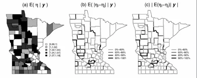
The global smoothing model of this subsection can be easily fit in WinBUGS; see for example the code available at www.biostat.umn.edu/~brad/ software.html. We applied this model to our Minnesota breast cancer dataset and here describe our results. Figure 2(a) maps posterior estimates of η, the relative risks, while Figure 2(b) does the same for the theoretical boundary likelihood values ∆ij. Figure 2(c) reverses the

order of the expectation and absolute value in (6), to see if this will better distinguish counties with differing variability but similar average absolute difference levels. The map of Eˆ (η|y) looks smoother and shows fewer discordant patches than the raw SLDR map in Figure 1(a).Also the ∆ij

posterior means seem to be somewhat better connected than the map based on the raw data in Figure 1(b). Panels (b) and (c) generally indicate boundary segments separating the southern and

Figure 2. Globally smoothed posterior summaries, breast cancer late detection data.

∆ij= |ηi-ηj|, for all iadjacent to j.

(5)

Eˆ (∆ij|y) =

1 G

Σ

(g)₌1 G

Σ

(g)_-η

j(g)|

(6)

G

g=1 g=1

G

pˆ_ij=Pr(∆_ij>c|y) = 1

G

Σ

1

G

Σ

where 1{∆_ij(g)_{>c} equals 1 if} ∆

ij(g)>c,and 0 otherwise.

G

g=1

northeast “arrowhead” regions from the remainder of the state.

Regarding the spatially-varying screening covariate, while its coefficient is consistent with intuition (posterior mean 0.0035; counties with higher nonscreening rates have higher late detection rates), it does not emerge as significantly different from 0 (95% posterior confidence limits -0.0022 and 0.0090).This means that the boundaries determined by the posterior mean of ∆ij(g) =|ηi - ηj| essentially follow the

smoothed late detection rates, not the screening covariates in Figure 1(c).The boundaries in Figures 2(b) and (c) resemble those in Figure 1(b), but the boundary segments are still mostly disconnected and overall patterns remain difficult to see.

Local areal smoothing and boundary detection

In the global smoothing (iid) model of the previous subsection, two counties with similar expected counts will contribute equally to the smoothed RR estimates of any other county. This may not be appropriate, since areas that are spatially closer together may tend to be more similar than areas that are further apart. This suggests some modification of the independence assumption in our extra-Poisson variability. Although spatial similarity in the data will lead to nonzero posterior correlations among RR estimates even under the iid model, we may prefer to incorporate this knowledge explicitly into the modeling through the distribution on the random effects φi.

To do this, we follow a common practice in areal data analysis, namely modeling the random effects φ=(φ1...,φn)’ using a conditionally

autoregressive (CAR)distribution [22]. The CAR

model smoothes the data according to a certain neighborhood structure specified in an n x

nproximity matrix, W, whose elements wij

measure “closeness” or adjacency of each pairof regions (i,j). The model corresponds to a joint spatial distribution for the areal random effects having joint density proportional to ,

where τ_φ is a positive scale parameter and Dw =

Diag(wi+) = Diag(

Σ

distribution as CAR(τ_φ,W). This density is awkward to work with (and may not even be proper; see below), but its full conditional

distributions have the form

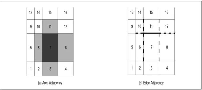
The most common choice for W is the 0-1 adjacency matrix illustrated in Figure 3(a).That is, we set wij= 1 if and only if j=/i(a region cannot be

a neighbor of itself) and regions i and j share a boundary; otherwise wij= 0. In this case we have

wi+=mi the number of neighbors for region i, so

the conditional distribution in (7) becomes quite intuitive, having mean φ−i, the average of the

neighboring φj, and variance decreasing in mi.The

model will thus encourage local smoothing of areal rates toward those of neighboring counties, with counties having more neighbors subject to a greater degree of smoothing. In Figure 3(a), the dark square (Region 7) has 4 neighbors (Regions 3, 6, 8, and 11, shaded light gray). Note that diagonally adjacent areas are unshaded; we only

Figure 3. Illustration of areal and edge domain neighborhood structures: (a) areal neighborhood structure; (b) edge neighborhood structure.

exp(– τφ

2φ’(Dw- W)φ),

φi|φj=/i~ N(

Σ

(7)

1

τφw_i+

w_ijφ_j

wi+

consider two areas to be adjacent if they share a common boundary of positive length. Boundary analysis can be implemented here via the Bayesian approach of Lu and Carlin [23], using posterior means or exceedance probabilities based on the

∆ijas described above.

While 0-1 adjacency matrices are most common in practice, the CAR remains a valid distributional specification for many other choices of W, providing myriad possibilities for spatial smoothing [24]. We might choose wij inversely

proportional to the distance separating the centroids of regions iand j, or even try to estimate

W from the data, possibly with the help of covariates [25,26].

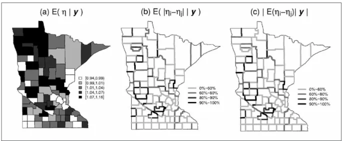
Figure 4 offers an analysis of the breast cancer data analogous to that in Figure 2, but assuming a locally smoothing 0-1 CAR prior for the random effects ϕ. Panel (a) greatly clarifies the overall spatial trend (higher late detection rates in the northwestern part of the state, lower in the northeast and south), but again suggests a collection of relative risks that are all close to 1.0. The 95% Bayesian confidence interval for the CAR smoothing parameter τis (29.1, 378.8), consistent with the degree of smoothing. Panels (b) and (c) show wombled maps analogous to those in Figure 2(b) and (c); again there is some evidence of spatial smoothing and a tendency toward better connected boundaries.

Local edge smoothing and boundary detection

In boundary analysis, we are interested in finding edges across which areal units are significantly different. Up until now our statistical model has been placed on data arising from the areal units themselves, with final boundaries arising from these (globally or locally) smoothed estimates.Although such methods are sensible for

areal rate estimation, they are less so for boundary analysis, since they do not directly model the edge variables and thus often do not deliver well-connected boundaries. As such, we now instead propose to model directly in the “edge domain”, where the basic data elements arise from the edges (boundary segments) themselves. With suitable modification, our existing iid and CAR models can be applied on this domain, leading (in the CAR case) to better-connected boundaries and easier map interpretation.

Starting with data collected over areal units, we need to define corresponding “observations” in the edge domain that capture the difference between neighboring units. A number of metrics could be used to measure this difference. When observed areal responses are univariate, the absolute difference |Yi-Yj| offers a sensible

definition. For multivariate areal responses, we can either use a multivariate summary or sums of univariate summaries; see the next section for further discussion.

If the original responses observed over the n

regions are counts, we first calculate the age-adjusted expected counts as in (3), and then take

as our edge-specific data values. The log transfor-mation helps stabilize the variability and produce a more symmetric and roughly normal empirical distribution for the collection of Uijon the real line.

For our statistical model on the edge domain, we assume

The variance is simply an intuitively sensible choice (more populous counties contribute to

Figure 4. Locally smoothed posterior summaries, breast cancer late detection data.

Uij= log

|

|

Yi Yj

Ei Ej

less uncertain Uij) inspired by previous work in

this area [27] and delta method approximations [1 p.159]. The inclusion of Yiand Yjin the variance

incorporates the different degrees of precision associated with the observed data.

Next, let

where xij is a vector of “discrepancy” covariates.

These may correspond to known edges created by mountain ranges, lakes, or other natural boundaries or the absolute differences of variables suspected to be important in causing inhomogeneity in Y

[25,26].The random effects ψijmodel residual edge

effects. Larger absolute ψij values indicate larger

discrepancies between the adjacent regions after accounting for the effects of the covariates.

To encourage the model to favor continuous boundaries, we use a CAR(λ,W*)prior for ψ,

where W* is a fixed adjacency matrix for the edges. Edge adjacency is essentially the dual problem of areal adjacency. To elucidate this duality, consider the edge neighborhood structure illustrated in Figure 3(b).The dark solid boundary corresponding to edge (7,11) has six “neighboring” edges, highlighted as dashed lines. Thus edge segments are adjacent if and only if they connect to one another. Note that (6,10) and (8,12) are neighbors of (7,11), even though these segments have no areal units in common. In order to create the edge adjacency matrix W*, we would first reindex each of the edge pairs from (i,

j) to a single index k running from 1 to nadj, the

total number of edges (area adjacencies) in the map.We then simply use the ordinary 0-1 format, with two edges kand 1 having W*klonly if they are

distinct and adjacent in the Figure 3(b) sense; otherwise W*kl= 0.

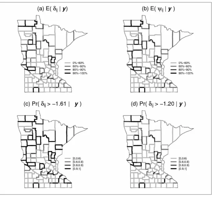
Figure 5. Posterior boundaries obtained via local edge smoothing, breast cancer late detection data.

Writing U_{= {Uij}, significant boundary segments}

may now be selected based on the absolute values of the posterior estimates E(δij |U), or based on

the exceedance probability approach using

P(δij>c|U) for some constant c. If interest lies in

identification of boundaries of abrupt changes after

accounting for covariate effects (residual-based

boundaries), we could select boundary segments based on posterior summaries of the ψijinstead.

Like the areal smoothing models above, posterior estimates based on our edge smoothing model can be easily fitted in WinBUGS; again see www.biostat.umn.edu/~brad/software.html. Figure 5 presents the results for the breast cancer late detection data.We use the absolute difference of screening rate as the lone covariate xij in (8),

even though its coefficient did not emerge as significantly different from 0 when included in the previous models. Panels (a) and (b) are the maps based on the posterior means of δijand ψij,

respectively.They are very similar, confirming that the inclusion of the mammography covariate has little impact on the results. Panels (c) and (d) are exceedance probability maps for δij using two

values of c that correspond on the log scale to SLDR differences of 0.2 and 0.3, respectively. The resulting maps are not scale-free, and differ from those shown in Figures 2 and 4 using the iid and areal CAR models, respectively, in their selection of many more northwestern boundary segments.

Summary and future work

Efforts to summarize geographic patterns from administrative data using maps are widespread. A limitation of such efforts and an ongoing source of criticism is the sometimes ad hoc way of grouping areas, a failure to explicitly recognize the spatial association inherent in administrative data, and the inability to consider multivariate relationships. The approach we have presented can be applied in a relatively straightforward manner to administrative data that are grouped to the zip code, county, or even state level.The ability to control for the inconsistent effects that are the result of small denominators (such as in rural areas) or small numerators due to relatively uncommon conditions (the annual incidence of breast cancer is 1%) is a key feature. Our group has applied this approach to studies of geographic availability of home-based health services with considerable success. Other applications would include studies of the impact of market structures on choice of service, as well as assessing the impact of an environmental factor that might influence disease incidence (such as studies of the impact of air or water quality).

Our local edge smoothing suggestion extends the idea of neighborhood structure modeling to the edge domain, as a more direct attack on the problem of areal boundary analysis. Like most CAR model implementations, our neighborhood structures were assumed constant (i.e., the proximity matrices W and W* were fixed in advance). In practice researchers typically model two areas as adjacent if they share a common boundary. But factors other than this could also impact the “closeness” between two geographically adjacent areas, such as the length of shared boundaries, the geographical topology near the boundaries, similarity of sociodemographic covariates such as race, level of urbanization, and so on. Future work looks toward development of approaches that allow estimation of the neighborhood structure itself, using both the value of the process in each area and other covariates that may indicate the inherent closeness between any two areas.

In this paper we restricted our attention to boundary analysis for a single response variable. When we have multivariate areal data (say, counts of p>2 outcomes over the same regions), correlation across response variables may occur if they share the same set of (spatially distributed) risk factors, or if they are linked by etiology, a common risk factor, or system of care. Moreover, the presence of one outcome might encourage or inhibit the presence of another over that same region. In this setting, traditional wombling methods use a metric to summarize the observations using a multivariate dissimilarity score. Thus the multivariate problem is transformed to a univariate problem. Another approach would be to treat the multivariate problem as related univariate problems and carry out spatial boundary analysis for each. In the first approach, we obtain a single set of boundaries, while in the second, multiple sets are obtained via Bayesian hierarchical multivariate CAR (MCAR) modeling [28,29]. Several basic MCAR models are easily fit in the WinBUGS package.

Acknowledgements

References

1) Banerjee S, Carlin BP, Gelfand AE. Hierarchical Modeling and Analysis for Spatial Data. Boca Raton, FL: Chapman and Hall/CRC Press, 2004.

2) Robinson WS. Ecological correlations and the behavior of individuals.Am Sociol Review 1950;15:351-7.

3) Gotway CA,Young LJ.Combining incompatible spatial data. J Am Statist Assoc 2002;97:632-48.

4) Sui DZ.Tobler’s first law of geography: a big idea for a small world? Ann Assoc Am Geographers 2004;94(2):269-77. 5) Dent BD. Cartography: Thematic Map Design. New York: William C. Brown/McGraw Hill, 1999.

6) Manton KE,Woodbury MA, Stallard E, Riggan WB, Creason JP, Pellom AC. Empirical Bayes procedures for stabilizing maps of U.S. cancer mortality rates. J Am Statist Assoc 1989;84:637-50. 7) Pickle LW, Mungiole M, Jones GK, White AA. Atlas of United States Mortality. Hyattsville, MD: National Center for Health Statistics, 1996.

8) Mungiole M, Pickle LW, Simonson KH. Application of a weighted headbanging algorithm to mortality data maps. Statistics in Medicine 1999;18:3201-9.

9) Womble WH.Differential systematics.Science 1951;114:315-22. 10) Gelfand AE, Smith AFM. Sampling-based approaches to calculating marginal densities. J Am Statist Assoc 1990;85:398-409. 11) Carlin BP, Louis TA. Bayes and Empirical Bayes Methods for Data Analysis, 2nd ed. Boca Raton, FL: Chapman and Hall/CRC Press, 2000.

12) Akaike H.Information theory and an extension of the maximum likelihood principle. In: Petrov BN, Csàki F editors. 2nd Intl. Symp. on Information Theory. Budapest: Akadèmiai Kiadò, 1973:267-81.

13) Schwarz G. Estimating the dimension of a model. Ann Statist 1978;6:461-4.

14) Spiegelhalter DJ, Best N, Carlin BP, van der Linde A. Bayesian measures of model complexity and fit (with discussion). J Roy Statist Soc 2002;SerB, 64:583-639.

15) Gelman A, Carlin JC, Stern H, Rubin DB. Bayesian Data Analysis, 2nd ed. Boca Raton, FL: Chapman and Hall/CRC Press, 2004. 16) Gilks WR, Richardson S, Spiegelhalter DJ editors. Markov chain Monte Carlo in Practice. London: Chapman and Hall, 1996.

17) Boscoe, FP, Pickle LW. Choosing geographic units for choropleth rate maps, with an emphasis on public health applications. Cartography and Geographic Information Science 2003;30:237-48.

18) Thomas A, Carlin BP. Late detection of breast and colorectal cancer in Minnesota counties: an application of spatial smoothing and clustering. Statistics in Medicine 2003;22:113-27. 19) Collette HJ, de Waard F, Rombach JJ, Collette C, Day NE. Further evidence of benefits of a (non-randomised) breast cancer screening program:The DOM project. J Epidem Comm Health, 1992;46:382-6.

20) Berry DA. Benefits and risks of screening mammography for women in their forties: a statistical appraisal. J Nat Cancer Inst 1998;90:1431-9.

21) Taplin SH, Ichikawa L, Yood MU, et al. Reason for late-stage breast cancer: absence of screening or detection, or breakdown in follow-up? J Nat Cancer Inst 2004;96(20):1518-27.

22) Besag, J. Spatial interaction and the statistical analysis of lattice systems (with discussion). J Roy Statistic Soc 1974;Ser. B, 36 :192-236.

23) Lu H, Carlin BP. Bayesian areal wombling for geographical boundary analysis. Geographical Analysis 2005;37:265-85. 24) Cressie NAC. Statistics for Spatial Data, 2nd ed. New York: Wiley, 1993.

25) Lu H, Banerjee S, Reilly C, Carlin BP. Bayesian areal wombling via adjacency modeling. Environmental and Ecological Statistics 2006 (in press).

26) Ma H, Carlin BP, Banerjee S. Hierarchical and joint site-edge methods for Medicare hospice service region boundary analysis. Research report, Division of Biostatistics, University of Minnesota, 2006.

27) Short M, Carlin BP, Bushhouse S. Using hierarchical spatial models for cancer control planning in Minnesota (United States). Cancer Causes and Control 2002;13:903-16.

28) Gelfand AE, Vounatsou P. Proper multivariate conditional autoregressive models for spatial data analysis. Biostatistics 2003;4:11-25.