Investing for the Long Run when Returns
Are Predictable
NICHOLAS BARBERIS*
ABSTRACT
We examine how the evidence of predictability in asset returns affects optimal portfolio choice for investors with long horizons. Particular attention is paid to estimation risk, or uncertainty about the true values of model parameters. We find that even after incorporating parameter uncertainty, there is enough predictability in returns to make investors allocate substantially more to stocks, the longer their horizon. Moreover, the weak statistical significance of the evidence for predictabil-ity makes it important to take estimation risk into account; a long-horizon investor who ignores it may overallocate to stocks by a sizeable amount.
ONE OF THE MORE STRIKING EMPIRICAL F INDINGS in recent financial research is
the evidence of predictability in asset returns.1In this paper we examine the
implications of this predictability for an investor seeking to make sensible portfolio allocation decisions.
We approach this question from the perspective of horizon effects: Given the evidence of predictability in returns, should a long-horizon investor al-locate his wealth differently from a short-horizon investor? The motivation for thinking about the problem in these terms is the classic work of Sam-uelson ~1969! and Merton~1969!. They show that if asset returns are i.i.d., an investor with power utility who rebalances his portfolio optimally should choose the sameasset allocation, regardless of investment horizon.
In light of the growing body of evidence that returns are predictable, the investor’s horizon may no longer be irrelevant. The extent to which the ho-rizondoes play a role serves as an interesting and convenient way of think-ing about how predictability affects portfolio choice. Moreover, the results may shed light on the common but controversial advice that investors with long horizons should allocate more heavily to stocks.2
* Graduate School of Business, University of Chicago. I am indebted to John Campbell and Gary Chamberlain for guidance and encouragement. I also thank an anonymous referee, the editor René Stulz, and seminar participants at Harvard, the Wharton School, Chicago Business School, the Sloan School at MIT, UCLA, Rochester, NYU, Columbia, Stanford, INSEAD, HEC, the LSE, and the London Business School for their helpful comments.
1See for example Keim and Stambaugh
~1986!, Campbell~1987!, Campbell and Shiller~1988a, 1988b!, Fama and French~1988, 1989!, and Campbell~1991!.
2See Siegel
~1994!, Samuelson~1994!, and Bodie~1995!for some recent discussions of this debate.
On the theoretical side, it has been known since Merton~1973!that vari-ation in expected returns over time can potentially introduce horizon effects. The contribution of this paper is therefore primarily an empirical one: Given actual historical data on asset returns and predictor variables, we try to understand the magnitude of these effects by computing optimal asset allo-cations for both static buy-and-hold and dynamic optimal rebalancing strategies.
An important aspect of our analysis is that in constructing optimal port-folios, we account for the fact that the true extent of predictability in returns is highly uncertain. This is of particular concern in this context because the evidence of time variation in expected returns is sometimes weak. A typical example is the following.3Letr
tbe the continuously compounded real return
on the value-weighted portfolio of the New York Stock Exchange in montht, and ~d0p!t be the portfolio’s dividend-price ratio, or dividend yield, defined
as the sum of dividends paid in monthst211 throughtdivided by the value of the portfolio at the end of month t. An OLS regression of the returns on the lagged dividend yield, using monthly returns from January 1927 to De-cember 1995, gives
rt5 20.005610.2580
S
d p
D
t211et, ~0.0064! ~0.1428!
~1!
where standard errors are in parentheses and the R2 is 0.0039.
The coefficient on the dividend yield is not quite significant, and theR2 is
very low. Some investors might react to the weakness of this evidence by discarding the notion that returns are predictable; others might instead ig-nore the substantial uncertainty regarding the true predictive power of the dividend yield and analyze the portfolio problem assuming the parameters are known precisely. We argue here that both of these views, though under-standable, are f lawed. The approach in this paper constitutes what we be-lieve is an appropriate middle ground: The uncertainty about the parameters, also known asestimation risk, is accounted for explicitly when constructing optimal portfolios.
We analyze portfolio choice in discrete time for an investor with power utility over terminal wealth. There are two assets: Treasury bills and a stock index. The investor uses a VAR model to forecast returns, where the state vector in the VAR can include asset returns and predictor variables. This is a convenient framework for examining how predictability affects portfolio choice: By changing the number of predictor variables in the state vector, we can compare the optimal allocation of an investor who takes return predict-ability into account to that of an investor who is blind to it.
How is parameter uncertainty incorporated? It is natural to take a Bayes-ian approach here. The uncertainty about the VAR parameters is summa-rized by the posterior distribution of the parameters given the data. Rather
3Kandel and Stambaugh
~1996!use a similar example to motivate their related work on portfolio choice.
than constructing the distribution of future returns conditional on fixed pa-rameter estimates, we integrate over the uncertainty in the papa-rameters cap-tured by the posterior distribution. This allows us to construct what is known in Bayesian analysis as the predictive distribution for future returns, con-ditional only on observed data, and not on any fixed parameter values. By comparing the solution in the cases where we condition on fixed parameters, and where we integrate over the posterior, we see the effect of parameter uncertainty on the portfolio allocation problem.
Our first set of results relates to the case where parameter uncertainty is ignored – that is, the investor allocates his portfolio taking the parameters as fixed at their estimated values in equation ~1!. We analyze two distinct portfolio problems: a static buy-and-hold problem and a dynamic problem with optimal rebalancing.
In the buy-and-hold case, we find that predictability in asset returns leads to strong horizon effects: an investor with a horizon of 10 years allocates significantly more to stocks than someone with a one-year horizon. The rea-son is that time-variation in expected returns such as that in equation ~1!
induces mean-reversion in returns, lowering the variance of cumulative re-turns over long horizons. This makes stocks appear less risky to long-horizon investors and leads them to allocate more to equities than would investors with shorter horizons.
We also find strong horizon effects when we solve the dynamic problem faced by an investor who rebalances optimally at regular intervals. However, the results here are of a different nature. Investors again hold substantially more in equities at longer horizons, but only when they are more risk-averse than log utility investors. The extra stock holdings of long-horizon investors are “hedging demands” in the sense of Merton ~1973!. Under the specifica-tion given in equaspecifica-tion~1!, the available investment opportunities change over time as the dividend yield changes: When the yield falls, expected returns fall. Merton shows that investors may want to hedge these changes in the opportunity set. In our data, we find that shocks to expected stock returns are negatively correlated with shocks to realized stock returns. Therefore, when investors choose to hedge, they do so by increasing their holdings of stocks.
As argued earlier, it may be important that the investor take into account uncertainty about model parameters such as the coefficient on the predictor variable in equation~1!, or the regression intercept. The standard errors in equation ~1! indicate that the true forecasting ability of the dividend yield may be much weaker than that implied by the raw parameter estimate. The investor’s portfolio decisions can be improved by adopting a framework that recognizes this.
We find that in both the static buy-and-hold and the dynamic rebalancing problem, incorporating parameter uncertainty changes the optimal alloca-tion significantly. In general, horizon effects are still present, but less prom-inent: A long-horizon investor still allocates more to equities, but the magnitude of the effect is smaller than would be suggested by an analysis using fixed parameter values. In some situations, we find that uncertainty about
pa-rameters can be large enough to reverse the direction of the results. Instead of allocating more to stocks at long horizons, investors may actually allocate less once they incorporate parameter uncertainty properly.
Though parameter uncertainty has similar implications for both buy-and-hold and rebalancing investors, the mechanism through which it operates differs in the two cases. Incorporating uncertainty about the regression in-tercept and about the coefficient on the predictor variable increases the vari-ance of the distribution for cumulative returns, particularly at longer horizons. This makes stocks look riskier to a long-term buy-and-hold investor, reduc-ing their attractiveness. In the case of dynamic rebalancreduc-ing, the investor needs to recognize that he will learn more about the uncertain parameters over time; we find that the possibility of learning can also reduce the stock allocation of a long-term investor, possibly to a level below that of a short-horizon investor. The lower allocation to stocks serves as a hedge against changes in perceived investment opportunities as the investor updates his beliefs about the parameters.
Parameter uncertainty also affects the sensitivity of the optimal allocation to the predictor variable. When it is ignored, the optimal allocation to stocks is very sensitive to the value of the dividend yield: If the yield falls, predict-ing low stock returns, the investor lowers his allocation to stocks sharply. Behavior of this kind makes for a highly variable allocation to stocks over time. When we acknowledge that the parameters are uncertain, the alloca-tion becomes less sensitive to changes in the dividend yield, leading to more gradual shifts in portfolio composition over time.
There is surprisingly little empirical work on portfolio choice in the pres-ence of time-varying expected returns. To our knowledge, Brennan, Schwartz, and Lagnado ~1997! make the first attempt on this problem. Working in continuous time, they analyze the dynamic programming problem faced by an investor who rebalances optimally, for a small number of assets and pre-dictor variables. Their approach is to solve the partial differential equation derived originally by Merton ~1973! for this problem. Motivated by their results, Campbell and Viceira ~1999! are able to find an analytical approx-imation to the more general problem of deriving both optimal consumption and portfolio rules for an infinite-horizon investor with Epstein–Zin utility. Kim and Omberg~1996!make a related theoretical contribution by deriving exact analytical formulas for optimal portfolio strategies when investors have power utility and expected returns are governed by a single mean-reverting state variable. All these papers ignore estimation risk.
The issue of parameter uncertainty was first investigated by Bawa, Brown, and Klein ~1979! in the context of i.i.d. returns.4 Kandel and Stambaugh ~1996! were the first to point out the importance of recognizing parameter uncertainty in the context of portfolio allocation with predictable returns. Using a Bayesian framework similar in spirit to ours, they show that for a short-horizon investor, the optimal allocation can be sensitive to the current
4Other papers in this vein include Jobson and Korkie
~1980!, Jorion~1985!, and Frost and Savarino~1986!.
values of predictor variables such as the dividend yield, even though regres-sion evidence for such predictability may be weak. By examining a wider range of horizons, both short and long, rather than the one-month horizon of Kandel and Stambaugh~1996!, we hope to uncover a broader set of phenom-ena and a more substantial role played by parameter uncertainty.
Section I introduces the framework we use for incorporating predictability and parameter uncertainty into the optimal portfolio problem. Sections II and III construct distributions for long-horizon returns, and use them to solve a buy-and-hold investor’s portfolio problem. The focus is on how these distributions and the resulting optimal allocation are affected by predict-ability and parameter uncertainty. Rather than introduce both effects at once, we bring them in one at a time: Section II considers parameter uncer-tainty in the context of an i.i.d. model; Section III then allows for predict-ability. Section IV turns to the dynamic problem of optimal rebalancing and contrasts the results with those in the buy-and-hold case. We analyze esti-mation risk in a dynamic context, including the possibility of learning more about the parameters over time. Section V concludes.
I. A Framework for Asset Allocation
This section presents a framework for investigating how predictability in asset returns and uncertainty about model parameters affect portfolio choice. The framework is based on that of Kandel and Stambaugh ~1996!, who in turn draw on models originally proposed by Zellner and Chetty~1965!. Since much of our analysis focuses on investors with long horizons, it is important to be precise about the choices these investors are allowed to make. We distinguish between three different ways of formulating the portfolio problem. One possibility is a buy-and-hold strategy. In this case, an investor with a 10-year horizon chooses an allocation at the beginning of the first year, and does not touch his portfolio again until the 10 years are over.
The second strategy, we call myopic rebalancing. In this case, the investor chooses some arbitrary rebalancing interval, say one year for the 10-year investor. He then chooses an allocation at the beginning of the first year, knowing that he will reset his portfolio to thatsameallocation at the start of every year. This is myopic in that the investor does not use any of the new information he has once a year has passed.
The final, most sophisticated strategy is optimal rebalancing. Assume again that the rebalancing interval is one year. In this case, the investor chooses his allocation today, knowing that at the start of every year, he will reopti-mize his portfolio using the new information at each time.
This paper presents results for both the buy-and-hold and the optimal rebalancing cases. The results for myopic rebalancing are too similar to those for the buy-and-hold strategy to justify reporting them separately. In the next few paragraphs, we describe the asset allocation framework from the perspective of a buy-and-hold investor. We postpone a detailed discussion of the dynamic rebalancing problem until Section IV; most of the issues de-scribed below, however, remain highly relevant for that case as well.
A. Asset Allocation Framework for a Buy-and-Hold Investor
Suppose we are at time T and want to write down the portfolio problem for a buy-and-hold investor with a horizon of TZ months. There are two as-sets: Treasury bills and a stock index. For simplicity, we suppose that the continuously compounded real monthly return on Treasury bills is a con-stantrf. We model excess returns on the stock index using a VAR framework
similar to that in Kandel and Stambaugh ~1987!, Campbell~1991!, and Ho-drick ~1992!. It takes the form
zt5a1Bxt211et, ~2!
with zt' 5~rt,xt'!, xt 5~x1,t, . . . ,xn,t!', and et; i.i.d. N~0,S!. The first
com-ponent ofzt, namelyrt, is the continuously compounded excess stock return
over montht.5The remaining components ofz
t, which together make up the
vector of explanatory variablesxt, consist of variables useful for predicting
returns, such as the dividend yield. This VAR framework therefore neatly summarizes the dynamics we are trying to model. The first equation in the system specifies expected stock returns as a function of the predictor vari-ables. The other equations specify the stochastic evolution of the predictor variables.
If initial wealth WT 51 and v is the allocation to the stock index, then
end-of-horizon wealth is given by
WT1TZ 5~12v!exp~rfTZ !1vexp~rfTZ 1rT111 {{{ 1rT1TZ!. ~3!
The investor’s preferences over terminal wealth are described by constant relative risk-aversion power utility functions of the form
v~W!5
W12A
12A. ~4!
Writing the cumulative excess stock return over TZ periods as
RT1TZ 5rT111rT121{{{ 1rT1TZ, ~5!
the buy-and-hold investor’s problem is to solve
max
v ET
S
$~12v!exp~rfTZ!1vexp~rfTZ 1RT1TZ!%12A
12A
D
. ~6!5A portfolio’s “excess” return is defined as the rate of return on the portfolio minus the
ET denotes the fact that the investor calculates the expectation conditional on his information set at time T. At the heart of this paper is the issue of which distribution the investor should use in calculating this expectation. The distribution may be very different, depending on whether the investor accounts for parameter uncertainty or recognizes the predictability in returns. To see whether predictability in returns has any effect on portfolio choice, our strategy is to compare the allocation of an investor who recognizes pre-dictability to that of an investor who is blind to it. The VAR model provides a way of simulating investors with different information sets: We simply alter the number of predictor variables included in the vectorxt.
Once the predictors have been specified, a standard procedure is to esti-mate the VAR parametersu5~a,B, S!, and then iterate the model forward with the parameters fixed at their estimated values. This generates a dis-tribution for future stock returns conditional on a set of parameter values, which we write as p~RT1TZ6z,u!Z , where z5~z1, . . . ,zT!' is the data observed
by the investor up until the start of his investment horizon. The investor then solves
max
v
E
v~WT1TZ!p~RT1TZ6z,u!Z dRT1TZ. ~7!The problem with this approach is that it ignores the fact that u is not known precisely. There may be substantial uncertainty about the regression coefficients a and B. For a long-horizon investor in particular, it is impor-tant to take the uncertainty in the estimation—estimation risk—into ac-count. A natural way to do this is to use the Bayesian concept of a posterior distributionp~u6z!, which summarizes the uncertainty about the parameters
given the data observed so far. Integrating over this distribution, we obtain the so-called predictive distribution for long-horizon returns. This distribu-tion6is conditioned only on the sample observed, and not on any fixed u:
p~RT1TZ6z!5
E
p~RT1TZ6u,z!p~u6z!du. ~8!A more appropriate problem for the investor to solve is then max
v
E
v~WT1TZ!p~RT1TZ6z!dRT1TZ. ~9!This framework allows us to understand how parameter uncertainty af-fects portfolio choice. We simply compare the solution to problem~7!, which ignores parameter uncertainty, with the solution to problem~9!, which takes this uncertainty into account.
6It is clearly an abuse of notation to use the same notationpfor all the different
How can problems ~7! and ~9! be solved? We calculate the integrals in problems~7!and~9!forv50, 0.01, 0.02, . . . ,0.98, 0.99, and report thevthat maximizes expected utility. Throughout the paper, we restrict the allocation to the interval 0# v #1, precluding short selling and buying on margin.7
The integrals themselves are evaluated numerically by simulation. To il-lustrate the idea behind simulation methods, imagine that we are trying to evaluate
E
g~y!p~y!dy,where p~y! is a probability density function. We can approximate the inte-gral by
1 I i
(
51I
g~y~i!!
,
wherey~1!, . . . ,y~I!
are independent draws from the probability density p~y!. To ensure a high degree of accuracy, we take I51,000,000 throughout.
In the examples considered in this paper, the conditional distribution p~RT1TZ6z,u! is Normal. Therefore the integral in equation ~7! is
approxi-mated by generating 1,000,000 independent draws from this Normal distri-bution, and averaging v~WT1TZ! over all the draws.
In the case of equation~9!, it is helpful to rewrite the problem as
max
v
E
v~WT1TZ!p~RT1TZ,u6z!dRT1TZ du5max
v
E
v~WT1TZ!p~RT1TZ6z,u!p~u6z!dRT1TZ du.~10!
The integral can therefore be evaluated by sampling from the joint dis-tributionp~RT1TZ,u6z!, and then averagingv~WT1TZ!over those draws. As the
decomposition in equation~10!shows, we sample from the joint distribution by first sampling from the posterior p~u6z! and then from the conditional
p~RT1TZ6z,u!. Sections II and III give detailed examples of this.8
7To be exact, we restrict the allocationv to the range 0#v#0.99. We do not calculate
expected utility for v51 because in this case the integral in equation ~9!equals 2`. The
problem is that whenv51, wealth can be arbitrarily close to zero, but the left tail of the predictive distribution does not shrink fast enough to ensure that expected utility is bounded from below.
8The integral in problem
~7!is only one dimensional and therefore quadrature methods are a reasonable alternative to simulation. This is not the case for problem~9!. To write down a closed-form expression for p~RT1TZ6z!, we would need to integrate out the parameters u, as
shown in equation~8!, and this is not possible forTZ.1. We therefore need to integrate over the parameter space as well, and an integral of this size can only be tackled by simulation. For the
This section has shown how to vary the degree of predictability observed by the investor—by changing the set of predictor variables included in the re-gression model—and how to incorporate parameter uncertainty into the analy-sis, by integrating over the posterior distribution of the parameters. Sections II and III use this framework to examine how the optimal portfolio changes when predictability in returns and estimation risk are accounted for.
B. The Data
The empirical work in this paper uses postwar data on asset returns and predictor variables. The stock index is the value-weighted index of stocks traded on the NYSE, as calculated by the Center for Research in Security Prices~CRSP!at the University of Chicago. In calculating excess returns, we use U.S. Treasury bill returns as provided by Ibbotson and Associates. We also use the dividend yield as a predictor variable. The dividend yield in month t is defined as the dividends paid by the firms in the stock index during monthst211 throught, divided by the value of the index at the end of month t.
Monthly data are used throughout, spanning 523 months from June 1952 through December 1995. We restrict the data to this postwar period so as to avoid the time before the Treasury Accord of 1951 when interest rates were held almost constant by the Federal Reserve Board. Since the regression attempts to model the stochastic behavior of stock returns in excess of Trea-sury bills, it is important to avoid structural breaks in the time series for the latter variable.
II. The Effect of Parameter Uncertainty
Rather than incorporate both predictability and parameter uncertainty at once, we introduce them one at a time. That is, we start out by considering the special case of the model in Section I where no predictor variables are included in the VAR—and hence where asset returns are i.i.d.—and look at how parameter uncertaintyalone affects portfolio allocation. In Section III, we move to the more general case which allows for predictability in returns. A. Constructing the Predictive Distribution
Suppose then that stock index returns are i.i.d., so that
rt5m1et, ~11!
where rt is the continuously compounded excess return on the stock index
over month t, and where et;i.i.d. N~0,s 2
!.
special case ofTZ51, the parametersucanbe integrated out, giving a closed-formt-distribution for the one-period-ahead predictive distribution. The integral is therefore again one dimen-sional and can be accurately handled by quadrature. By looking only at theTZ51 case, Kandel and Stambaugh~1996!are able to take advantage of this.
As described in Section I, a buy-and-hold investor with a horizonTZ months long starting at time T solves the problem stated in equation ~6!. In our numerical work, we setrf, the continuously compounded real monthly T-bill return, equal to 0.0036, the real return on T-bills over December 1995, the last month of our sample.9
The investor has two choices of distribution for calculating the expecta-tion in equaexpecta-tion ~6!. He may incorporate parameter uncertainty and use the predictive distribution for returns p~RT1TZ6r!, where r 5 ~r1, . . . ,rT!.
Alternatively, he may ignore parameter uncertainty and calculate the ex-pectation over the distribution of returns conditional on fixed parameter values,p~RT1TZ6r,m,s2!. The effect of parameter uncertainty is revealed by
comparing the optimal portfolio allocations in these two cases.
We approximate the integral for expected utility by taking a sample
~RT1TZ ~i!
!ii551I from one of the two possible distributions, and then computing
1 I i
(
51I $~12v!exp~r
fTZ!1vexp~rfTZ 1RT1TZ ~i!
!%12A
12A . ~12!
In Section II.B, we present the optimal allocations vwhich maximize ex-pression~12!for a variety of risk aversion levelsAand investment horizons
Z
T, and for each of the two cases where the investor either ignores or ac-counts for parameter uncertainty. Since sampling from the distributions p~RT1TZ6r!and p~RT1TZ6r,m,s2! is an important step in computing these
op-timal allocations, we devote the next few paragraphs to explaining the sam-pling procedure in more detail.
As indicated in equation ~10!, there are two steps to sampling from the predictive distribution for long-horizon returns p~RT1TZ6r!. First, we
gener-ate a large sample from the posterior distribution for the parameters p~ m,s26r!. Second, for each of the ~ m,s2! pairs drawn, we sample once
from the distribution of long-horizon returns conditional on both past data and the parameters, p~RT1TZ6m,s2,r!, a Normal distribution. This produces
a large sample from the predictive distribution. We now provide more de-tail about each of these steps.
To construct the posterior distribution p~ m,s26r!, a prior is required.
Throughout this section, we use a conventional uninformative prior,10
p~ m,s2! @
1
s2.
9The nominal return on T-bills in December 1995 is def lated using the rate of change in the
Consumer Price Index, provided by Ibbotson and Associates.
10Another reasonable approach would be to use a more informative prior that puts zero
weight on negative values ofm, ref lecting the observation in Merton~1980!that the expected market risk premium should be positive.
Zellner ~1971!shows that the posterior is then given by
s26r;IG
S
T21 2 ,
1 2 t
(
51T
~rt2rS!2
D
m6s2,r;NS
rS,s2
T
D
, where rS 5 ~10T!(
t51T
rt.
To sample from the posterior p~ m,s26r!, we therefore first sample from
the marginal p~s26r!, an Inverse Gamma distribution, and then, given the s2 drawn, from the conditionalp~ m6s2,z!, a Normal distribution. Repeating
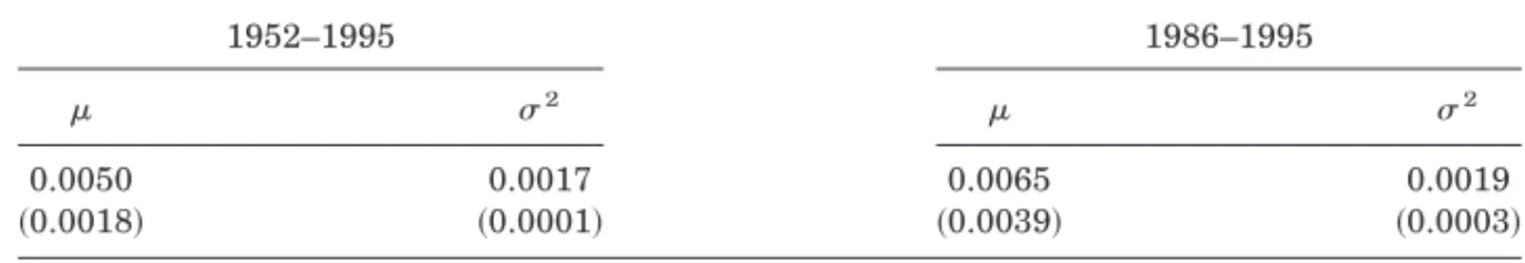
this many times gives an accurate representation of the posterior distribution. Table I presents the results of this procedure. The left panel uses monthly data on stock index returns from June 1952 to December 1995. The right panel uses the subsample of data from January 1986 to December 1995. An investor who believes that the meanmand variances2 of stock returns are changing over time may feel more comfortable estimating those parameters over this second more recent data sample.
In each case, the data are used to generate a sample of size 1,000,000 from the posterior distribution formands2. Table I gives the mean and standard deviation of the posterior distribution for each parameter. For example, for an investor using the full sample from 1952 to 1995, the posterior distribu-tion for the mean monthly excess stock return mhas mean 0.005 and stan-dard deviation 0.0018. This appears to be an important source of parameter uncertainty for the investor. The posterior distribution for the variances2is much tighter and is centered around 0.0017. An investor confining his at-tention to the shorter data set will be more uncertain about the parameters; the standard deviation of the posterior form is now a substantial 0.0039.
Table I
Parameter Estimates for an i.i.d. Model of Stock Returns
The results in this table are based on the model rt5m 1et, wherert is the continuously
compounded excess stock index return in monthtandet;i.i.d.N~0,s
2
!. The table gives the mean and standard deviation~in parentheses!of each parameter’s posterior distribution. The left panel uses data from June 1952 to December 1995; the right panel uses data from January 1986 to December 1995.
1952–1995 1986–1995
m s2 m s2
0.0050 0.0017 0.0065 0.0019
The second step in sampling from the predictive distribution is to sample from the distribution of returns conditional on fixed parameter values p~RT1TZ6m,s2,r!. Since
rT115m1eT11,
I ~13!
rT1TZ 5m1eT1TZ,
the sumRT1TZ 5rT111rT121 . . . 1rT1TZ is Normally distributed conditional
onmands2with meanTZmand varianceTZs2. Therefore, for each of the 1,000,000 pairs ofm ands2 drawn from the posterior p~ m,s26r!, we sample one point
from the Normal distribution with meanTZmand varianceTZs2. This gives a sample of size 1,000,000 from the predictive distributionp~RT1TZ6r!, which we
can use to compute the optimal allocation when taking parameter uncertainty into account.
Our strategy for understanding the effect of parameter uncertainty is to compare the allocation of an investor who uses the predictive distribution when forecasting returns with the allocation of an investor who ignores es-timation error, sampling instead from the distribution of returns conditional on fixed parameters p~RT1TZ6r,m,s2!. For the latter case, we assume that
the investor takes the posterior means of m and s2 given in Table I as the fixed values of the parameters, and then draws 1,000,000 times from a Nor-mal distribution with mean TZm and variance TZs2.
We are now ready to present optimal portfolio allocations. We compute the quantity in equation ~12! for v ranging from zero to 0.99 in increments of 0.01, and report the vmaximizing this quantity. The procedure is repeated for several possible investment horizons, ranging from one year to 10 years in one-year increments, for several values of risk aversionAand for the two possible distributions for cumulative returns, one of them ignoring estima-tion risk, the other incorporating it.
B. Results
Figure 1 shows the optimal percentage 100vpercent allocated to the stock index, plotted against the investment horizon in years. The upper graphs show the optimal allocations chosen by investors who use the full data set from 1952 to 1995; the lower graphs are for investors who use only the subsample from 1986 to 1995. The two graphs on the left are based on a risk-aversion of A5 5, those on the right are for A510. The dash0dot line
shows the allocation conditional on fixed parameter values, and the solid line shows the allocation when we account for parameter uncertainty.
The dash0dot line is completely horizontal in all the graphs. In other words,
an investor ignoring the uncertainty about the mean and variance of asset returns would allocate the same amount to stocks, regardless of his invest-ment horizon. This sounds similar to Samuelson’s famous horizon irrele-vance result, although it is important to note that the two results are different. Samuelson~1969! shows that with power utility and i.i.d. returns, the
opti-mal allocation is independent of the horizon. However, he proves this for an investor who optimally rebalances his portfolio at regular intervals, rather than for the buy-and-hold investor we consider here.
The main point of this exercise though, is to show how the allocation dif-fers when parameter uncertainty is explicitly incorporated into the inves-tor’s decision-making framework. Interestingly, Figure 1 shows that in this case, the stock allocationfalls as the horizon increases. In other words, pa-rameter uncertainty can introduce horizon effects even within the context of an i.i.d. model for returns. This point does not appear to have been noted in the earlier literature on this topic, such as Bawa et al.~1979!. That research focuses more on how estimation risk varies with the size of the data sample, while keeping the investor’s horizon fixed. The results here are concerned with the effects of estimation risk as we vary the investor’s horizon, while keeping the sample size fixed.
The magnitude of the effects induced by parameter uncertainty are sub-stantial. For an investor using the full data set, and with A55, the differ-ence in allocation at a 10-year horizon is approximately 10 percent. For another
Figure 1. Optimal allocation to stocks plotted against the investment horizon in years.
The investor follows a buy-and-hold strategy, uses an i.i.d. model for asset returns, and has power utility W12A
0~12A!over terminal wealth. The dash0dot line corresponds to the case
where the investor ignores parameter uncertainty, the solid line to the case where he accounts for it. The top two graphs use data from 1952 to 1995, the lower two use data from 1986 to 1995.
investor with the same risk-aversion of A5 5, but who uses only the more recent subsample of data, the effect is dramatically larger, a full 35 percent at the 10-year horizon! This ref lects the greater impact of the higher pa-rameter uncertainty faced by an investor who uses such a short data sample. The fact that parameter uncertainty makes a difference is often confusing at first sight. When parameter uncertainty is ignored, the investor uses a Normal distribution with meanTZmand variance TZs2 for his forecast of log cumulative returns. Both the mean and, more importantly, the variance, grow linearly with the investor’s horizonT. Figure 1 shows that this leads toZ the same stock allocation, regardless of the investor’s horizon.
Accounting for estimation risk changes this. The investor’s distribution for long-horizon returns now incorporates an extra degree of uncertainty, increasing its variance. Moreover, this extra uncertainty makes the variance of the distribution for cumulative returns increase fasterthan linearly with the horizonT. This makes stocks look riskier to long-horizon investors, whoZ therefore reduce the amount they allocate to equities.
The reason variances increase faster than linearly with the horizon is because, in the presence of parameter uncertainty, returns are no longer i.i.d. from the point of view of the investor, but rather positively serially correlated. To understand this more precisely, recall that an important source of uncertainty in the parameters surrounds the mean of the stock return. If the stock return is high over the first month, then it will probably be high over the second month because it is likely that the state of the world is one with a high realization of the uncertain stock mean parameterm. This is the sense in which stock returns are positively serially correlated from the in-vestor’s perspective.
An important issue we have not yet discussed is the accuracy of the nu-merical methods used to obtain the optimal portfolios. In an effort to main-tain high accuracy, we use samples conmain-taining 1,000,000 draws from the sampling distribution when calculating expected utility. In the Appendix, we attempt to convey the size of the simulation error that is present; the results there suggest that using 1,000,000 draws does indeed provide a high degree of accuracy.
III. The Effect of Predictability
A. Constructing the Predictive Distribution
Now that the impact of parameter uncertainty alone has been illustrated, predictability can be introduced as well. We return to the regression model of equation ~2! discussed in Section I. In the calculations presented in this section, the vector zt contains only two components: the excess stock index
returnrt, and a single predictor variable, the dividend yieldx1,t, which
cap-tures an important component of the variation in expected returns.11
11Many papers demonstrate the dividend yield’s ability to forecast returns. See for example
As explained in Section I, the problem faced at time Tby a buy-and-hold investor with a horizon of TZ months is given by equation ~6!. There are a number of possible distributions the investor can use when computing the expectation in equation ~6!. An investor who ignores the uncertainty in the model parameters uses the distribution of future returns conditional on both past data and fixed parameter valuesu,p~RT1TZ6u,z!, wherez5~z1, . . . ,zT!'.
In contrast, the investor who takes parameter uncertainty into account sam-ples from the predictive distribution, conditional only on past data and not on the parameters, p~RT1TZ6z!.
We approximate the integral for expected utility by taking a sample
~RT1TZ ~i!
!ii551I from one of the two possible distributions, and then computing
1 I i
(
51I $~12v!exp~r
fTZ!1vexp~rfTZ 1RT1TZ ~i!
!%12A
12A . ~14!
In Section III.B we present the optimal allocationsvwhich maximize the quantity in expression~14!for a variety of risk aversion levelsAand invest-ment horizonsT, and for different cases where the investor either ignores orZ accounts for parameter uncertainty. The next few paragraphs explain how we sample fromp~RT1TZ6z!andp~RT1TZ6u,z!, an important step in computing
these optimal allocations.
The procedure for sampling from the predictive distribution is similar to that in Section II. First, we generate a sample of sizeI51,000,000 from the posterior distribution for the parametersp~a,B,S6z!. Second, for each of the
1,000,000 sets of parameter values drawn, we sample once from the distri-bution of returns conditional on both past data and the parameters, a Nor-mal distribution. This gives us a sample of size 1,000,000 from the predictive distribution for returns, conditional only on past returns, with the param-eter uncertainty integrated out. We now provide more detail about each of these steps.
To compute the posterior distribution p~a,B,S6z!, rewrite the model as
1
z2' IzT'
2
5
1
1 x1'
1 I
1 xT'21
2
S
a'B'
D
1
1
e2' I eT'
2
, ~15!
or
Z5XC1E, ~16!
where Z is a ~T 21,n11! matrix with the vectors z2', . . . ,zT' as rows; X is
a ~T21,n11!matrix with the vectors ~1x1'!, . . . ,~1xT'21! as rows, and Eis
a ~T 2 1,n1 1! matrix with the vectors e2', . . . ,e
T' as rows. Finally C is an ~n 11,n 11! matrix with top row a'
and the matrix B'
below that. Here n 51 because we use only one predictor variable, the dividend yield.
Zellner ~1971! discusses the Bayesian analysis of a multivariate regres-sion model in the traditional case with exogenous regressors. His analysis carries over directly to our dynamic regression framework with endogenous regressors; the form of the likelihood function is the same in both cases, so long as we condition on the first observation in the sample, z1. A standard
uninformative prior here12 is
p~C,S!@ 6S62~n12!02.
The posteriorp~C,S216z! is then given by
S21
6z;Wishart~T2n22,S21! vec~C!6S,z;N~vec~CZ!,SJ~X'X!21!
where S5 ~Z2 XCZ !'~Z2 XCZ! with CZ 5 ~X'X!21X'Z. We sample from the
posterior distribution by first drawing from the marginalp~S216z!, and then
from the conditional p~C6S,z!.
Table II presents the mean and standard deviation of the posterior distri-bution for a, B, and S, generated by sampling 1,000,000 times from that posterior. The left panel uses the full data sample covering the period 1952
12Stambaugh
~1999!discusses the use of alternative priors and of using the unconditional likelihood instead of conditioning onz1.
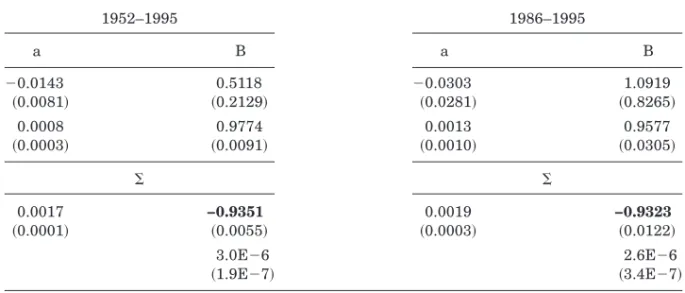
Table II
Parameter Estimates for a VAR Model of Stock Returns
The results in this table are based on the modelzt5a1Bxt211et, wherezt5~rt xt!'includes
continuously compounded monthly excess stock returnsrtand the dividend yieldxt, and where
et;i.i.d.N~0,S!. The table gives the mean and standard deviation~in parentheses!of each
parameter’s posterior distribution. The figures in bold above the diagonal in the variance ma-trices are correlations. The left panel uses data from June 1952 to December 1995; the right panel uses data from January 1986 to December 1995.
1952–1995 1986–1995
a B a B
20.0143 0.5118 20.0303 1.0919
~0.0081! ~0.2129! ~0.0281! ~0.8265!
0.0008 0.9774 0.0013 0.9577
~0.0003! ~0.0091! ~0.0010! ~0.0305!
S S
0.0017 −0.9351 0.0019 −0.9323
~0.0001! ~0.0055! ~0.0003! ~0.0122!
3.0E26 2.6E26
to 1995; the results on the right are obtained using the subsample from 1986 to 1995. An investor who believes that the relationship between the dividend yield and stock returns is changing over time may prefer to estimate the regression over this more recent sample.
Look first at the left panel of Table II. The B matrix shows the well-documented predictive power of the dividend yield for stock returns: The posterior distribution for that coefficient has mean 0.5118 and standard de-viation 0.2129. The dividend yield is highly persistent. The variance matrix shows the strong negative correlation between innovations in stock returns and the dividend yield, estimated here at 20.9351; this has an important inf luence on the distribution of long-horizon returns. Note also the greater parameter uncertainty faced by investors using only the recent subsample; in particular, the predictive power of the dividend yield for returns is now estimated much less accurately.
The second step in sampling from the predictive distribution is to sample fromp~RT1TZ6u,z!. Note that sincezt5a1Bxt211«t, we can writezt5a1
B0zt211 «t where
B05
3
1
0
I
0
2
B4
.Therefore
zT115a1B0zT1eT11
zT125a1B0a1B02zT1eT121B0eT11 I
zT1TZ 5a1B0a1B02a1 {{{ 1B0TZ21a
1B0TZzT
1eT1TZ 1B0eT1TZ211B02eT1TZ221 {{{1B0TZ22eT121B0TZ21eT11. ~17!
Conditional on a, B, and S, the sum ZT1TZ 5 zT111zT12 1{{{1zT1TZ is
Normally distributed with mean and variance given by
msum5TaZ 1~TZ 21!B0a1~TZ 22!B02a1 {{{1B0TZ21a
1~B01B021 {{{1B0TZ!zT,
~18!
Ssum5 S
1~I1B0!S~I1B0!'
1~I1B01B02!S~I1B01B02!' ~19!
I
For each of the 1,000,000 realizations of the parameters in the sample from the posterior p~a,B,S6z!, we draw one point from the Normal
distri-bution with mean and variance given by the above expressions, thereby giv-ing a sample of size 1,000,000 from the predictive distribution.
The aim of this section is to understand how predictability in asset re-turns and parameter uncertainty affect portfolio choice. To do this, we com-pute optimal allocations using four different choices for the distribution of future returns. These distributions differ in whether they take into account predictability and parameter uncertainty. For instance, the investor may choose to take predictability into account when forecasting returns. He does so by including the dividend yield in the VAR he uses to forecast returns. Alternatively, he may ignore the predictability in returns simply by exclud-ing the dividend yield from the VAR. In this case, the model for returns reduces to the i.i.d. model of Section II.
So far, this gives two different ways of forecasting future returns. How-ever, for each of these two ways, there is a further choice to be made. The investor may account for the parameter uncertainty in the model, and use a predictive distribution constructed in the manner described earlier. Alterna-tively, he may ignore the parameter uncertainty in the model; in this case, we assume that the distributions for future returns are constructed using the posterior means ofa,B, andSgiven in Table II~or ofmands2 in Table I if predictability is also ignored! as the fixed values of the parameters, and then drawing 1,000,000 times from the Normal distribution with mean and variance given by equations ~18! and ~19! above. This extra choice about whether to incorporate parameter uncertainty gives a total of four possibil-ities for the distribution of future returns.
In Section III.B below, we present optimal portfolio allocations. We eval-uate the quantity in equation ~14! forvranging from zero to 0.99 in incre-ments of 0.01, and report thevmaximizing this quantity. We do this calculation for several values of investor risk-aversion A; for several investment hori-zons, ranging from one year to 10 years at one-year intervals; and for the four possible distributions for future returns. By comparing how the optimal portfolios differ depending on which distribution we use for forecasting re-turns, we can understand how the predictive power of the dividend yield and parameter uncertainty affect portfolio choice.13
The investor’s distribution for future returns of course depends on the value of the dividend yield at the beginning of the investment horizon,x1,T.14
If the yield is low, this forecasts low returns, lowering the mean of the dis-tribution for future returns and reducing the allocation to equities. In our initial set of results, we abstract from this effect by setting the initial value of the dividend yield to its mean in the sample, namelyx1,T53.75 percent,
and investigate how the optimal allocation changes with the investor’s ho-13The optimal portfolios for the cases where predictability is ignored are computed in
Sec-tion II, so we simply carry those results over to this secSec-tion.
14The initial value of the predictorx
rizon for this fixed initial value of the predictor. Later, we look at how the results are affected when the initial dividend yield takes values above or below its sample mean.
B. Results
Figure 2 presents the solutions to the allocation problem. Each graph cor-responds to a different level of risk-aversion. Within each graph, each line shows the percentage 100v percent allocated to stocks plotted against the investment horizon ranging from one to 10 years. The four lines on each graph correspond to the four possible distributions the investor could use to forecast future returns.15All of the computations are based on the full data
sample from 1952 to 1995; results based on the more recent subsample are presented in Section III.C.
We focus on the graph for a risk aversion level of 10, which presents the results most clearly. The two lower lines in this graph represent the cases where the investor ignores predictability, excluding the dividend yield from the VAR. Of course, in this case, the model for returns simply reduces to the i.i.d. model discussed in Section II. These two lines are therefore exactly the same as those in the top right graph in Figure 1.
The main results of this section center on the two upper lines. These two lines correspond to the cases where the dividend yield is included in the analysis. The graph shows that when we ignore uncertainty about the model parameters ~the dashed line!, the optimal allocation to stocks for a long-horizon investor is much higher than for a short-long-horizon investor. When we take the uncertainty about the parameters into account ~the solid line!, the long-horizon allocation is again higher than the short-horizon allocation— but not nearly as much higher as when we ignore estimation risk. The rest of this section explores these results in more detail.
We start with the case where parameter uncertainty is ignored. Why does the allocation to stocks in this case rise so dramatically at long horizons when the dividend yield is included in the regression?
Recall that when asset returns are modeled as i.i.d., the mean and vari-ance of cumulative log returns grow linearly with the investor’s horizon T.Z In Section II, we find that this leads to identical allocations to stocks, re-gardless of the investor’s horizon.
When we acknowledge that returns may be predictable rather than i.i.d., this is no longer the case. The variance of cumulative log stock returns may grow slower than linearly with the investor’s horizon, making stocks look relatively less risky at longer horizons and hence leading to higher alloca-tions to stocks in the optimal portfolio.
15Sometimes, the optimal allocation 100
vpercent lies outside the~0,100!range for all ho-rizons between one and 10 years, which is why there may be fewer than four lines on some graphs.
This point can be seen mathematically. Write the regression model in full as
rt115a1bx1,t1«1,t11 ~20!
x1,t115g1fx1,t1«2,t11, ~21!
where
S
«1,t «2,tD
;N
S
0,S
s12 s12 s12 s22
DD
.
Figure 2. Optimal allocation to stocks plotted against the investment horizon in years.
The investor follows a buy-and-hold strategy, uses a VAR model which allows for predictability in returns, and has power utilityW12A
0~12A!over terminal wealth. The solid and dotted lines
correspond to cases where the investor accounts for uncertainty in the parameters, the dashed and dash0dot lines to cases where he ignores it. The solid and dashed lines correspond to cases
where the investor takes into account the predictability in returns, the dotted and dash0dot
The conditional variances of one- and two-period cumulative stock returns are
varT~rT11!5s12, ~22!
varT~rT111rT12!52s121b2s2212bs12. ~23!
For the parameter values estimated from the data, in other words the posterior means in Table II,b2s2212bs12, 0, which implies that the
con-ditional variance of two-period returns is less than twice the conditional variance of one-period returns. When we consider the predictive power of the dividend yield, conditional variances grow slower than linearly with the investor’s horizon, lowering the perceived long-run risk of stocks and in-creasing their optimal weight in the investor’s portfolio.
Some numbers may help to make this point clearer. Table I shows that the variance of monthly excess stock returns is estimated at 0.0017, implying a standard deviation of %0.0017 5 4.12 percent. In a model specifying
i.i.d. returns, this implies a standard deviation for cumulative log excess returns over 10 years of~0.0412!%120545.2 percent. However, the standard
deviation of the distribution for 10-year cumulative log excess returns gen-erated by an investor who models returns using the VAR in Table II, ignor-ing parameter uncertainty, is from equation~19!equal to 23.7 percent, much lower than 45.2 percent! This demonstrates the extent to which conditioning on the dividend yield can slow the evolution of the variance of cumulative returns.
The intuition behind this effect is the following: Suppose that the dividend yield falls unexpectedly. Sinces12, 0, this is likely to be accompanied by a contemporaneous positive shock to stock returns. However, since the divi-dend yield is lower, stock returns are forecast to belowerin the future, since
b . 0. This rise, followed by a fall in returns, generates a component of negative serial correlation in returns which slows the evolution of the vari-ance of cumulative returns as the horizon grows.
The results obtained here should not be viewed as being specific to the particular way we have modeled returns, nor to the particular parameter values estimated from the data. There is a strong economic intuition behind the general idea that time variation in expected returns induces mean-reversion in realized returns. If there is a positive shock to expected returns, it is very reasonable that realized returns should suffer a contemporaneous negative shock since the discount rate for discounting future cash f lows has suddenly increased. This negative shock to current realized returns, fol-lowed by the higher returns predicted in the future, are the source of mean-reversion, which in turn makes stocks more attractive to long-run investors. While mean-reversion provides a simple way of interpreting our results, it is important to note that horizon effects can be present even without nega-tive serial correlation in returns. In other words, the predictability in
re-turns may be sufficient to make stocks more attractive at long horizons, without being strong enough to induce mean-reversion in returns. One way to see this is to note that in our simplified model,
cov~rt,rt11!5
b2fs22
12f2 1bs12 ~24!
cov~rt,rt1i!5fi21cov~rt,rt11!. ~25!
It is straightforward to note that we can choose parameters so that re-turns are serially uncorrelated at all lags and yet, by equation ~23!, the two-period conditional variance is less than twice the one-period conditional variance. In this situation, a two-period investor would allocate more to stocks than a one-period investor and yet there is no mean-reversion in returns.
The second important result in Figure 2 is that incorporating parameter uncertainty can substantially reduce the size of the horizon effect. ForA510, ignoring this uncertainty can lead to an overallocation to stocks of more than 30 percent at a 10-year horizon!
Introducing parameter uncertainty has a number of effects. First, the in-vestor acknowledges that he is uncertain about the mean stock return. In exactly the same way as in Section II, incorporating the uncertainty about the mean makes conditional variances grow more quickly as the horizon grows, tending to make stocks look more risky. Therefore the allocation to stocks is lower than in the case where estimation risk is ignored.
The investor also recognizes that the true predictive power of the dividend yield is uncertain; therefore it is also uncertain whether the dividend yield really does slow the evolution of conditional variances, and hence whether stocks really are less risky at long horizons. The investor is therefore again more cautious about stocks and allocates less to them.16
In the absence of estimation risk, we saw that predictability makes stocks look less risky at long horizons; incorporating the estimation risk makes them look more risky. These two effects therefore battle it out, leading to stock allocations that are not necessarily monotonic as a function of the investment horizon. The solid line in the bottom left graph in Figure 2 shows that for horizons up to eight years, predictability wins out and the allocation to stocks rises; from that point on, the line falls slightly, suggesting that estimation risk has caught up with the investor, making stocks look less attractive.
16When the investor takes estimation risk into account, he acknowledges both that the
predictive power of the dividend yield may be weaker than the point estimates suggest—in which case he would certainly be reluctant to allocate more to stocks at long horizons—andthat it may in fact be stronger, in which case he would be even keener to allocate more to equities at longer horizons. These effects go in opposite directions; on net, the investor invests less at long horizons because he is risk-averse and hence dislikes the mean-preserving spread that accounting for estimation risk adds to the distribution of future returns.
C. The Role of the Predictor Variable
Up to this point we have focused on just one effect of including the divi-dend yield as a predictor in the VAR. Conditioning on the dividivi-dend yield reduces the variance of predicted long-horizon cumulative returns, leading to a higher allocation to stocks for long-horizon investors.
Conditioning on the dividend yield has another, more direct implication for portfolio allocation. By its very nature as a predictor, the dividend yield also affects the mean of the distribution for future returns. When the divi-dend yield is low relative to its historical mean, an investor forecasts lower than average stock returns and hence reduces his allocation to stocks. This effect has not been prominent so far in the paper because the initial value of the dividend yield has been kept fixed at its unconditional mean in the sample period.
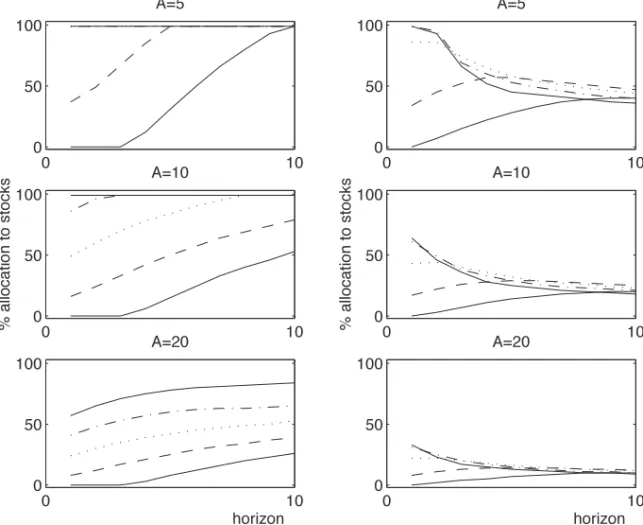
We now repeat the earlier analysis of this section for different initial val-ues of the dividend yield.17 Figure 3 presents the results. Each graph
cor-responds to a different level of risk aversion. The graphs on the left illustrate the optimal allocations when parameter uncertainty is ignored; the graphs on the right incorporate it. Within each graph, we plot the optimal stock allocation as a function of the investor’s horizon for five different initial values of the dividend yield. The five values we use are the historical mean of the dividend yield in our sample, namely x1,T 5 3.75 percent, and the
values one and two standard deviations on either side of that.18
Look first at the graphs on the left side of Figure 3. They show that for all the initial values of the predictor that we consider, the earlier result of this section continues to hold: The allocation to stocks rises with the investor’s horizon. Of course, for anyfixedhorizon, the optimal allocation is higher for higher values of the dividend yield since the investor expects higher future returns. For any fixed initial value of the dividend yield, however, the 10-year allocation is higher than the one-10-year allocation. Moreover, the optimal allocation of an investor with a 10-year horizon is just as sensitive to the initial value of the dividend yield as the optimal allocation of a one-year horizon investor. In other words, the allocation lines show no sign of converging.
The picture is remarkably different when the investor properly accounts for the fact that he is uncertain about the parameters governing asset re-turns. These results are shown in the graphs on the right-hand side of Fig-ure 3. For lower initial values of the dividend yield, the optimal allocation once again rises with the investor’s horizon. For higher values of the pre-dictor, though, the allocation to stocks falls with the investment horizon.
17In effect, we are producing optimal portfolio recommendations for an investor who has
observed a hypothetical sample with differentx1,T but the same posterior distribution for the
parameters as in the actual sample.
18For some of the initial values of the dividend yield, the optimal allocation 100
vpercent lies outside the~0,100!range for all horizons between one and 10 years. This is why there may be fewer than five lines on any one graph.
Another way of looking at this is to note that the allocation lines converge, resulting in a 10-year allocation that is less sensitive to the initial dividend yield than the allocation of a one-year investor, and much less sensitive than the allocation of an investor with a 10-year horizon who ignores estimation risk. This result is intuitive: If the true forecasting power of the dividend yield is uncertain, the allocation of a long-horizon investor should be less sensitive to the initial value of the predictor.
Though Figure 3 shows that the impact of parameter uncertainty is sub-stantial, its effect can be even more dramatic. Suppose that an investor be-lieves that the true predictive power of the dividend yield changes over time and is therefore wary of running a regression over the full 1952 to 1995 period, preferring instead to estimate the relationship over the shorter 10-year period from 1986 to 1995. The posterior distribution of the VAR pa-rameters over this data sample is summarized in Table II.
Figure 3. Optimal allocation to stocks plotted against the investment horizon in years.
The investor follows a buy-and-hold strategy, uses a VAR model which allows for predictability in returns, and has power utilityW12A
0~12A!over terminal wealth. The three graphs on the left
ignore parameter uncertainty, those on the right account for it. The five lines within each graph correspond to different initial values of the predictor variable, the dividend yield: d0p52.06
per-cent~solid!, d0p52.91 percent~dashed!, d0p53.75 percent~dotted!, d0p54.59 percent~dash0
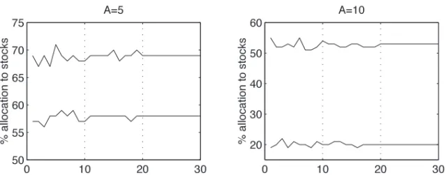
Figure 4 repeats the calculations of Figure 3 for the case where the inves-tor uses the more recent subsample in making his decisions. Once again, the optimal allocation rises sharply with the horizon for the investor who takes the parameters as fixed. When parameter uncertainty is incorporated, how-ever, the recommended portfolios are completely different! The allocations for investors with 10-year horizons are now largely insensitive to the initial value of the predictor: The convergence in the allocation lines, already pro-nounced in Figure 3, is now much more dramatic. Just as in Figure 3, esti-mation risk is sometimes so strong as to cause the stock allocation for a 10-year investor to be lower than that for a one-year investor. In this case, this is even true when the dividend yield is at its sample mean,x1,T53.36
percent!
Figure 4. Optimal allocation to stocks plotted against the investment horizon in years.
The investor follows a buy-and-hold strategy, uses a VAR model which allows for predictability in returns, and has power utilityW12A
0~12A!over terminal wealth. The three graphs on the
left ignore parameter uncertainty, those on the right account for it. The five lines within each graph correspond to different initial values of the predictor variable, the dividend yield: d0p5
2.37 percent~solid!, d0p52.86 percent~dashed!, d0p53.36 percent~dotted!, d0p53.85 percent ~dash0dot!, and d0p54.35 percent~solid!. The model is estimated over the 1986 to 1995 sample
Another intriguing result in Figures 3 and 4 is the fact that for a given investment horizon and risk-aversion level, the optimal stock allocation is not necessarily increasing in the initial value of the predictor variable. This is a surprising fact at first sight: If the initial value of the dividend yield is five percent rather than four percent, the distribution for future returns forecast by the investor has a higher posterior mean, which should lead to a higher allocation to the stock index. Moreover, the variance of the distribu-tion for future returns is insensitive to the initial value of the predictor, so this cannot explain the nonmonotonicity result. Stambaugh ~1999! demon-strates that it is in fact the third moment of the return distribution, skew-ness, that is important here. Incorporating parameter uncertainty generates positive skewness in the predictive distribution for low initial values of the predictor, and negative skewness for higher initial values. This negative skew-ness makes stocks less attractive, the higher the dividend yield, and makes the optimal allocation nonmonotonic in the initial value of the predictor.
A reader trying to interpret the results in Figures 2, 3, and 4 will obvi-ously be concerned about the accuracy of the numerical methods. As men-tioned at the end of Section II, the Appendix contains a discussion of simulation error. We do not dwell on it any more here, other than to say that the results there suggest that by using 1,000,000 draws in our simulations, we can be comfortable that the level of accuracy is high.
IV. Dynamic Allocation
To this point we have focused on the buy-and-hold investment problem. We now examine portfolio choice when the investor optimally rebalances over his investment horizon. Specifically, consider an investor who is al-lowed to rebalance annually using the new information at the end of each year. We analyze how the optimal allocation depends on the investor’s hori-zon. To begin, we work with the simpler case where parameter uncertainty is ignored. Then we look at how the results change when the investor incor-porates parameter uncertainty.
A. An Asset Allocation Framework with Dynamic Rebalancing
We use the same regression model as in Section III, originally introduced as equation~2!in Section I, withzt5~rt xt!', wherext5x1,tis the dividend
yield. We also maintain the earlier simplification that the continuously com-pounded real return on T-bills is a constant rf per period. As before, we set
rf 50.0036 in all our numerical work.
The investor who optimally rebalances his portfolio at regular intervals faces a dynamic programming problem. To solve this problem, we employ the standard technique of discretizing the state space and using backward in-duction. The next few paragraphs formalize this.
Suppose we are at timeT, and the investor has a horizon TZ months long. Divide the horizon intoKintervals of equal length,@t0,t1#,@t1,t2#, . . .@tK21,tK#,
respectively. The investor adjusts his portfolio Ktimes over the horizon, at points ~t0,t1, . . . ,tK21!. The control variables at the investor’s disposal are
~v0, . . . ,vK21!, his allocations to the stock index at times~t0, . . . ,tK21! respec-tively. To make the notation less cumbersome, we writeWkin place ofWtkfor
the investor’s wealth at timetk, zk in place ofztk, andxk in place ofxtk. The
investor’s problem is then
max
t0 Et0
S
WK 12A
12A
D
, ~26!where maxt0means that the investor maximizes over all remaining decisions from time t0 on, and where
Wk115Wk
H
~12vk!expS
rfZ
T
K
D
1vkexpS
rfZ
T
K 1Rk11
D
J
, ~27! Rk115rtk111rtk121 {{{1rtk11, ~28! for k 5 0, . . . ,K 2 1. Note that the return on T-bills between rebalancing points is now exp~rf~TZ0K!! because the fullTZ month horizon is broken intoKintervals. The cumulative excess stock return between rebalancing points tk and tk11 isRk11.
Define the derived utility of wealth
J~Wk,xk,tk!5max tk
Etk
S
WK 12A
12A
D
, ~29!where maxtkmeans a maximization over all remaining decisions from time
tk on. Note that the value functionJdoesnotdepend onrk, the stock return over monthtk, because in our model, the current value of the predictor vari-able alone characterizes the investment opportunity set. The Bellman equa-tion of optimality is
J~Wk,xk,tk!5max vk
Etk$J~Wk11,xk11,tk11!%. ~30!
A simple induction argument shows that derived utility may be written
J~Wk,xk,tk!5
Wk12A
12AQ~xk,tk!, ~31! forAÞ1, or in the case ofA51,