Aimyong_unc_0153D_14886.pdf

PROPENSITY SCORE METHODS FOR COMPETING RISKS

Natnaree Aimyong

A dissertation submitted to the faculty at the University of North Carolina at Chapel Hill in

partial fulfillment of the requirements for the degree of Doctor of Public Health in the

Department of Biostatistics in the Gillings School of Global Public Health.

Chapel Hill

2014

!

ABSTRACT

Natnaree Aimyong: Propensity Score Methods for Competing Risks

(Under the direction of Jason P. Fine and M. Alan Brookhart)

Non-experimental studies have increasingly been used to examine the safety and

effectiveness of medication. Challenges to this method include confounding, which may cause

the estimator to be biased. Propensity score (PS), which is the conditional probability of

receiving treatment given all confounders, may be used to control for confounding. Analysis of

vulnerable populations may involve competing risks, which may occur before the event of

interest. Statistical methods that account for competing risks are needed to obtain valid causal

estimate. However, little knowledge attention has been given to this topic in the literature.

The objective of this research was to investigate the performance of estimators under

implementation of various PS methods in competing risk survival analyses for estimating

marginal and conditional treatment effects. The competing risk models were a cause-specific

hazard model and subdistribution hazard model.

According to simulation results, the weighted method produced efficient estimators for

marginal treatment effects. However, it leads to an inflated variance when low incidence of event

and strong confounder effects. A bootstrapping method can be used to estimate the variance

under this scenario. For the conditional treatment effect, PS adjustment in the model performed

the best for the null model. Depending on the sample size and the number of confounding

variables, the subclassification and matching methods yield best performance under the

Heterogeneity of treatment effect associated with statin therapy may be present in el- derly

who experience myocardial infarction. Examining treatment effect across age groups and the

revascularization procedure illustrated the heterogeneity of statin effects. Statins significantly reduce

risks of heart failure among younger age groups. The combination of statins with revascularization

procedures presents better treatment effects than occurs with statins alone. Application of propensity

score methods to competing risks is illustrated in this study, with the analysis of treatment effects

providing an improved understanding of the heterogeneity of the effects of statins therapy.

The efficiency of implementing propensity score method to competing risks is illustrated in

this study. Analyzing the treatment effects by subgroup and medical procedure contributes better

I dedicate this work to all mothers, who always support,

ACKNOWLEDGMENTS

I wish to express sincere thanks to all who contributed many types of supports especially

the following:

First, I would like to thank Royal Thai Government for the scholarship they provided to me

and Mahidol University for the full scholarship and the partial scholarship I was awarded. I also

appreciate the support from the officers and staff of the Office of Educational Affairs of the

Royal Thai Embassy.

I would like to convey my gratefulness to Dr. Jason P. Fine for his excellent academic

guidance and inspiration beyond this dissertation. I also express my gratitude to Dr. M. Alan

Brookhart for his support and for introducing me to the field of Pharmacoepidemiology. Both of

them give me the opportunity to work in professional environment with kindness and patience. I

would like to thank my dissertation committee: Dr. Chirayath M. Suchindran, Dr. Richard

Bilsborro, Dr. Anastasia Ivanova and Dr. Todd Schwartz, for their valuable advice and

comments.

I am very grateful to my parents for their inspiration and courage. I am appreciative to all

friends for their help and support.

Last, I would like to express my appreciation to all of my teachers, instructors and

professors. They have all contributed to my store of knowledge, especially my kindergarten

TABLE OF CONTENTS

LIST OF TABLES………...

………x

LIST OF FIGURES………..

………xii

CHAPTER 1: Introduction……… ………1

1.1 Motivating Examples……… ………1

1.2 Causal Inference………..

………3

1.3 Propensity score and non-experimental studies………

………4

1.3.1 Matching……….. ………5

1.3.2 Subclassification……… ………7

1.3.3 Propensity score covariate adjustment………. ………7

1.3.4 Weighting……….. ………8

1.3.5 Variables selection for propensity score model………

………8

1.3.6 Assessment of the balance of the covariates………

………10

1.4 Marginal and conditional models………..

1………11

1.5 Competing risks model………..

………11

1.5.1 Notation………

………12

1.5.2 Latent failure times………

………12

1.5.3 Cause-specific hazard function………

………13

1.5.4 Subdistribution hazard function………

………13

1.7 Objective and outline………. ……..………15

CHAPTER 2: Marginal Treatment Effects of Completing Risks

Model………..….

….

...………….…………18

2.1 Introduction……….

……..………18

2.2 Methods……….. ……..………21

2.2.1 Monte Carlo simulation………. ……..………21

2.2.2 Simulation for subdistribution hazard function………. ……..………22

2.2.3 Simulation for cause-specific hazard function……….. …….…….………22

2.2.4 True marginal treatment effect……….. ……..………23

2.2.5 Propensity-based estimation of the treatment effect in

simulations………

…………..………24

2.2.6 Propensity-based estimation of the treatment effect in case

study………...

..………25

2.3 Monte Carlo simulation results………. …………..………25

2.3.1 True marginal treatment effects……… …………..………25

2.3.2 Propensity-based estimation performance……… …………..………26

2.4 Case study results………

…………..………30

2.5 Discussion……….. …………..………34

CHAPTER 3: Conditional Treatment Effects of Competing Risks

Models………..…

…………..………37

3.1 Introduction……….

…………..………37

3.2 Methods………..

…………..………38

3.2.1 Monte Carlo simulation……… …………..………38

3.2.2 Propensity-based estimation of the treatment effect in

simulations……….………40

3.3 Simulation results……….. ………..…………43

3.3.1 Under the null model………

………..…………43

3.3.2 Under the alternative model………

………44

3.4 Case study results……….. ………..…………49

3.5 Discussion……….. ………..…………51

CHAPTER 4: Application of Propensity Score methods for competing risks

under Heterogeneity………..…………

………53

4.1 Introduction……… ………..…………53

4.2 Method……… ………..…………56

4.2.1 Source of data and population………

…………..………56

4.2.2 Outcome and covariates………. …………..………56

4.2.3 Statistical analysis………. …………..………56

4.3 Results……….

………57

4.3.1 Propensity Score model………..

…………..………58

4.3.2 Treatment effects of statins for different age groups………

………59

4.3.3 Treatment effects of statins for patients who had a

revascularization procedure………..

…………..………64

4.4 Discussion……….. …………..………64

CHAPTER 5: Conclusion………

…………..………68

Appendix I: Propensity Score model………..

…………..………71

BIBLIOGRAPHY……… …………..………82

LIST OF TABLES

Table 1.1 Variables included into propensity score model...17

Table 2.1 True marginal treatment effect...26

Table 2.2 Simulation results of marginal treatment effect

using competing risks (sample size=500) ...27

Table 2.3 Simulation results of marginal treatment effect

using competing risks (sample size=2000)...28

Table 2.4 Number and percent of observed outcomes...30

Table 2.5 The treatment effects of statins for elderly who were

hospitalized for an AMI...32

Table 2.6 Comparison of the variance of the model-base

sandwich and bootstrapping method……….33

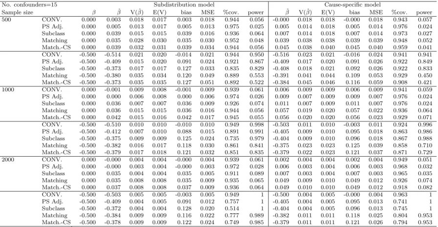
Table 3.1 Simulation result of conditional model of 5 confounders………..45

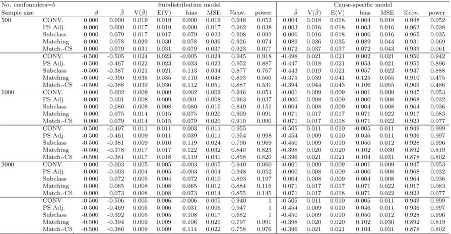
Table 3.2 Simulation result of conditional model of 15 confounders………46

Table 3.3 Simulation result of conditional model of 50 confounders………47

Table 3.4 Simulation result of conditional model of 100 confounders…...………...48

Table 3.5 The estimated treatment effects of statins from

conditional ...50

Table 4.1 Number and percent of observed events...58

Table 4.2 Results of treatment effects from the marginal, conditional risks

and competing risks models by age group...63

Table 4.3 Treatment effects of statins by status of revascularization procedure………...…65

Table 5.1 Propensity score model ...71

Table 5.2 Propensity score model by age groups...75

LIST OF FIGURES

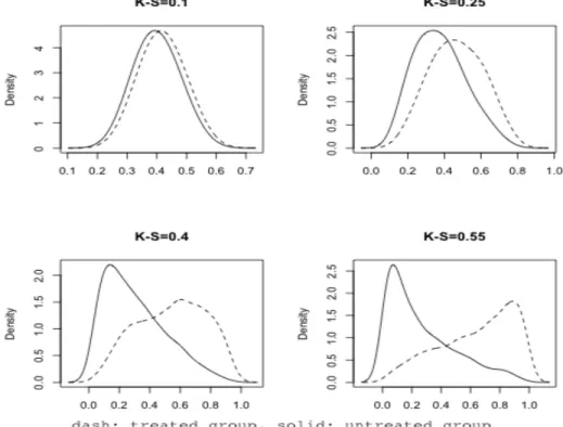
Figure 2.1 Density plots of treated and untreated group in four scenarios………26

Figure 4.1 Distribution of propensity score of statins users and non-users

by age group……….60

Figure 4.2 Distribution of propensity score of statins user and non-user

by revasucularization status ... 61

Figure 5.1 Distribution of the propensity score of statins users and non-users

Chapter 1

Introduction

1.1

Motivating Examples

Cardiovascular disease (CVD) is the leading cause of mortality and is a major cause

of morbidity in the United States and worldwide (108). Increasing steadily with age, the

prevalence of CVD events is even higher in the population older than 65 years of age,

a

ff

ecting more than 70% of both men and women and 66% of CVD deaths occur in people

age above 75 years old (92). As the population is aging, more people are likely to have

cardiovascular complications. Increasing attention has been drawn to the management

of CVD in the elderly population.

Non-experimental studies are increasingly used to evaluate the safety and e

ff

ective-ness of medications when used in usual clinical care (11). It is an appealing design for

investigation of statin treatment e

ff

ects among post MI patients. However, two major

challenges are present. The first challenge is presence of possible confounding systematic

di

ff

erences in prognosis between patients treated with statins and those untreated. If

left uncontrolled, the observed di

ff

erence in outcome risks cannot be interpreted as a

causal e

ff

ect solely due to statins. Another challenge is the presence of competing risks,

as the occurrence of some events may precede and thus preclude the occurrence of the

event of interest. In the elderly population after an acute MI, multiple comorbidities and

worsened health status put them at a higher risk of mortality. Death may thus preclude

the occurrence of the event of interest, (such as another MI) and make the evaluation

of the e

ff

ect of statins on MI di

ffi

cult. Sophisticated methods such as competing risks

survival analyses are needed in this setting (7, 64). Statistical methods that can account

for both competing risks and confounding are needed to obtain a valid causal estimate.

A competing risks survival analysis is a method to address the presence of multiple

events in a survival analysis of the time between the start of follow-up and either the

occurrence of the event(s) of interest or a censoring event (51). The outcomes of

compet-ing risk model are three mutually exclusive events includcompet-ing occurrence of the event of

interest, occurrence of a competing event, and a censoring event (lost to follow-up, end

of follow-up etc.). The regression models in competing risks may be used to estimate the

treatment e

ff

ects.

treatment e

ff

ects without relying on modeling the outcome, are an approach being

in-creasingly used in non-experimental studies (96).

Competing risk survival analyses with PS methods to control for confounding can then

be used to investigate e

ff

ect of statin treatment on cardiovascular events among post MI

patients. However, this approach has not been extensively explored, and little is known

about the performance of this approach compared to the existing standard methods. It is

of great interest to investigate the performance of competing risk models using propensity

score methods to control confounding for estimating marginal and conditional treatment

e

ff

ects.

1.2

Causal Inference

Causal inference is the process of drawing a conclusion about whether a causal

rela-tionship does in fact exist (43). Let

Yi(1) and

Yi(0) be the potential outcomes that would

have been observed for individual

i

in the treatment group or the control (untreated)

group, respectively. Individual causal e

ff

ects can then be obtained by contrasting the

values of the two potential outcomes. However, only one of the potential outcomes is

ob-served for each individual, thus, in general, individual causal e

ff

ects cannot be obtained.

Since it is generally impossible to identify individual causal e

ff

ects, an aggregated

causal e

ff

ect, the average causal e

ff

ect in a population of individuals, becomes the focus of

interest. Let

P

[Yz

= 1] be the counterfactual risk of outcome

Yz

, or the risk of developing

outcome

Y

in all subjects in the population receiving counterfactual treatment

z. An

average causal treatment e

ff

ect is present when

P

[Yz

= 1]

�

=

P

[Yz

= 1].

assumption is the independence of treatment assignment and outcomes conditional on

the covariates.

In randomized trials, only one potential outcome is observed for each individual.

However, the randomization process ensures that the balancing between the background

variables between treated and untreated groups. In other words, the randomization

pro-cess ensures the independent predictors of the outcome are equally distributed between

the treated and untreated groups. The treated and untreated groups are exchangeable,

and the exchangeability thus implies lack of confounding (65).

In non-experimental studies, treatment is not randomly assigned and the reason for

receiving treatment is likely to be associated with some predictors of the outcome. Thus,

exchangeability is not guaranteed. However, in weaker conditions, conditioning on many

pre-exposure covariates of the treated and untreated groups is often reasonable to allow

exchangeability. Let

L

be the confounding or background covariates. The conditional

exchangeability implies

P

[Y

= 1

|

L

= 1, Z

=

z] =

P

[Yz

= 1

|

L

=

l]

PS is the conceptual tool used to achieve accurate causal inference by balancing or

conditioning on the background variables of treated and untreated subjects (57).

1.3

Propensity score and non-experimental studies

validity of the treatment e

ff

ect estimated from non-experimental studies is a concern if

these biases are left uncontrolled.

Propensity score methods have emerged as a useful method to control for confounding

in the non-experimental setting. It is widely used in a variety of areas, including medical

(95), economic (42) and social research (67). The methods were formalized by Rosenbaum

and Rubin (80) and were shown to be able to control confounding. At the beginning,

the propensity score was developed to estimate the causal e

ff

ect of binary treatment

(48). A propensity score is the conditional probability of receiving treatment given all

confounders. Among patients with the same PS, treatment is unrelated to confounders.

Therefore, the two treatment groups have the same distribution of measured confounders.

The true propensity score of non-randomization studies is unknown. However, it can

be estimated from observed data. Statistical methods such as logistic regression and other

discriminant models can be used to estimate PS. Multivariable logistic regression is the

most widely used method for PS estimation. The estimation of the propensity score can

be implemented as a continuous variable via standard approaches including matching,

subclassification (stratification) by propensity score, propensity score adjustment to the

multivariate model, and weighting (96).

1.3.1

Matching

Matching on certain covariates to remove confounding by the matching variables

has been used extensively in cohort studies (96). Matching methods attempt to choose a

single or multiple patients from the untreated group with the same values of the matching

variables for each patient in the treated group. It can be easily implemented when

matching only needs to be done for a small number of covariates. A large number of

confounders in a non-experimental study makes matching on all confounders di

ffi

cult.

PS as a summary score reduces these multidimensional confounders to one dimension,

which helps overcome this limitation (19).

first option is nearest available matching on the estimated PS. The treated and

un-treated patients are first randomly ordered, and the first un-treated patient is matched with

the first untreated patient who has the nearest PS. The second option is Mahalanobis

metric matching (84). The Mahalanobis distance is the distance between two

dimen-sional points scaled by the statistical variation in each component of the point. Treated

and untreated patients are first randomly ordered, and then each treated patient is

pair-matched with the first untreated patient who has the closest Mahalanobis distance. The

third alternative is nearest available Mahalanobis metric matching within calipers defined

by PS. The treated group is first randomly ordered. For each treated patient, a group of

untreated patients are chosen given that the di

ff

erence of PS between the treated patient

and the untreated patient is less than the caliper (a constant value). From this group of

untreated patients, the patient who has the closest Mahalanobis distance to that of the

treated patient is selected as the match. The third matching method produces the best

balance for the covariate distributions between the treated and untreated groups and is

considered to outperform the first two.

The two popular algorithms for creating PS matched sets are greedy matching and

optimal matching . In greedy matching, a treated patient is first selected at random.

The untreated patient whose PS is closest to this patient is chosen as a match for this

patient. This process is repeated until all the untreated patients have been matched to all

the treated patients or when all the treated patients have been matched. In contrast to

the greedy matching, which finds the nearest untreated patient, optimal matching tries

to minimize the total within-pair distance di

ff

erences (83).

to have improved bias reduction. Full matching results in matched sets consisting of

ei-ther one treated patient and multiple untreated patients or one untreated patient and at

least one treated patient (77). Full matching removes bias better than pair matching and

may achieve the closer match than M:1 matching (37). However, fullmatching method

result in a wide range of ratio of treated to untreated patients (94).

In analyses using Cox proportional hazard models, PS pair-matching has been shown

to have the smallest amount of bias when compared to other methods (26, 4). Martens

showed the analysis from real data showed larger treatment e

ff

ects from matching and

subclassification compared to conventional Cox proportional hazard model (62).

1.3.2

Subclassification

Another method used to implement PS to control confounding is subclassification or

stratification of PS into equal-sized strata, estimation of the treatment e

ff

ect within these

strata and then combining the stratum-specific e

ff

ect estimates using a weighted-average

approach. Both treated and untreated groups are grouped into equal-sized strata based

on their PSs. In general, quintiles of PS are used to create the strata. Previous reports

have shown that subclassification into five strata can remove approximately 90% of initial

bias (81) despite the fact that it can also increase the variance of the estimator (104).

1.3.3

Propensity score covariate adjustment

Adding the PS to a multivariable outcome model is the least appealing method of PS

implementation, since the validity of this approach depends upon a correct specification

of both PS and outcome models. If the PS is included as a linear term in the outcome

model, an assumption is made that there is a linear relationship between the PS and the

outcome, which is likely to be violated in real world applications.

variances of the treated and untreated groups di

ff

er (19). When this method is applied

to studies using survival analysis to estimate e

ff

ects, the fixed parameters of the PS

vari-able suggest that the probability of receiving treatment given all measured covariates

has a constant e

ff

ect on the hazard ratio. Results from our simulation study showed

that the e

ffi

ciency of propensity score adjustment depended on the overlap area and the

specification of variables included into propensity score model (35).

1.3.4

Weighting

Standardization with weights generated from the PS can also be used to control

confounding. Unlike matching, this approach does not result in reduction of the original

sample size. Individuals within the original sample are weighted based on their PS to

create a pesudo-population where the covariates are well balanced in the two treatment

groups, and no association exists between the confounders and treatment. The weighting

method plays an importance role in the estimation of marginal treatment e

ff

ects. There

are two types of weighting commonly used: inverse probability of treatment weighted

(IPTW), standardized mortality ratio weighted (SMRW).

SMRW is set to one one for treated patients and defined as the ratio of the estimated

PS to one minus the estimated PS for the untreated (86). The untreated patients are thus

weighted to be representative of the treated population. The resulting e

ff

ect estimate

is generalizable to the treated population from which the observed treated sample was

drawn. Unlike PS matching, which also often estimates average treatment e

ff

ect in the

treated, no treated patients are excluded from the analysis.

In all weighting analyses, statistical methods are needed to account for the relation

between the replicated individuals created by the process of weighting. A robust sandwich

variance estimate is required to calculate the variance. This approach results in confidence

intervals that are conservative and wider than the nominal coverage.

Many studies have applied weighted methods to survival analysis. Cole and

Her-nan presented an approach to produce adjusted survival curves with inverse probability

weights which o

ff

ers direct interpretation of the data (16). Hernan et al (40) applied

IPTW to study zidovedine (AZT) treatment e

ff

ects on mortality and compared it to an

unweighted analysis. The weighted analysis showed that AZT reduced risks of mortality

but the unweighted analysis with a basic baseline adjustment model produced an adverse

e

ff

ect of AZT on mortality (which was contrary to reality).

Simulation studies showed survival analysis via Cox model with application of the

IPTW method produced the smallest amount of bias for the estimator of interest (4, 26).

1.3.5

Variables selection for propensity score model

the estimator of the average treatment e

ff

ect for the treated group when applying the

matching method and using a multinomial model for the outcome estimation (18, 110).

1.3.6

Assessment of the balance of the covariates

Once the PS model is fit, it is recommended to explicitly evaluate the performance of

the estimated PS model by assessing the balance of covariates after PS implementation

either through matching or weighting . Approaches to assess the covariate balance under

PS methods have been developed (3).

Evaluation of the lack of fit of the PS model is performed using the logistic regression

goodness-of-fit statistics and the c-statistic. the goodness of fit statistic summarizes the

deviation between the observed and predicted outcomes. The c-statistics value indicates

the capacity of a model to discriminate between treated subjects and untreated subjects

(46). However, both methods fail to detect the balancing of background variables between

treated and untreated groups (106).

1.4

Marginal and conditional models

A marginal treatment e

ff

ect is the average treatment e

ff

ect for the population, while a

conditional treatment e

ff

ect is the average treatment e

ff

ect for the individual (3). In the

absence of confounding, the di

ff

erence in means and risk di

ff

erence are collapsible, and the

conditional and marginal e

ff

ects are the same. In randomized studies, the covariates are

balanced between the two treatment groups, therefore the crude di

ff

erence in means and

the adjusted di

ff

erence in means will be equal. In non-experimental studies, the marginal

and conditional estimates will coincide if there was no unmeasured confounding, the

outcome was continuous, and the true outcome model was known (31). However, when

the outcome is either binary or time-to-event, and the odds ratio or the hazard ratio

is used as the e

ff

ect measure, then the marginal and conditional e

ff

ect will not coincide

even in the absence of confounders (34, 25).

For PS methods, the estimators from the conventional model (adjusting for

con-founders in the outcome regression model), covariate adjustment (adding the PS to a

multivariable outcome model) and matching method are estimating the conditional

treat-ment e

ff

ect. The PS based weighting methods yield estimates of the marginal treatment

e

ff

ect for the population.

1.5

Competing risks model

A survival analysis explores the time period from a certain point until the occurrence

of the event of interest. A competing risks survival analysis is the special case of survival

analysis where multiple events may occur and the occurrence of one event may preclude

the occurrence of the other. Competing risk events threaten the validity of studies, even

in randomized control trials. Individuals who are at higher risk of competing risk events

may be less likely to experience the absolute benefit of treatment (64). Care is needed

in statistical analysis to ensure that treatment e

ff

ects are appropriately quantified.

likelihood of the occurrence of a particular competing risk can be summarized using the

distribution of the observed data or using models representing the underlying mechanisms

that generated the observed data (54). When modeling the observed data, so-called crude

functions are utilized. The cause specific hazard and cumulative incidence functions

described below are the most widely used quantities. A popular mechanistic model

is the latent failure time model discussed below. The net function is the probability

of the occurrence of the event of interest corresponding to the latent failure time in

the hypothetical situation where the particular risk of event is the only risk present.

Additional properties of the crude and net approaches are now discussed.

1.5.1

Notation

For this discussion, the following notations are used. Let

Y

and

C

be failure and

censoring times, and

ε

∈

{

1,

2, ..J

}

be the failure event. For each individual

i, i=1,...,n,

the observed failure time was

Ti,

T

= (Y

∧

C), and the observed event be

ε

∆

ε

=

I(Y

≤

C) when I(

·

) is indicator function. Let

Z

be one for treated group and zero for untreated

group.

1.5.2

Latent failure times

There are J mutually exclusive types of failure events, and the corresponding time

until each failure type is

Tij

�

. The observed time is

minj

(

Tij

�

), with each

Tij

�

defined as

if the other causes were not present, and with the observed cause of failure

ε

being the

index of the observed latent failure time. The hazard function for latent failure times is

a net hazard function defined as:

�

λ

= lim

1

∆

t

P

(t

≤

Tij

�

< t

+

∆

t,

ε

=

j

|

Tij

�

≥

t), j

= 1, ..., J.

1.5.3

Cause-specific hazard function

To model competing risk using a cause-specific hazard function, the type-specific or

cause-specific hazard function is defined as:

hj

(t) = lim

1

∆

t

P

(t < T < t

+

∆

t,

ε

=

j

|

T

≥

t), j=1,...m.

The cause-specific hazard function is the instantaneous rate for a failure of type

j

at

time

t, in the presence of all other failure types (54). With this cause-specific hazard

function approach, an event

k

(k

�

=j) is censored at time

T

if events other than type

j

are

observed. The cumulative incidence function,

P

(T

_≤

t,

ε

=

j),which is the probability of

occurrence of event

j

at time

t

is defined as:

Fj

(t) =

�

0

hj(s)S(s)d

s

, where S is the survival function for T.

Defining

Si(t) to be the survival function based on

hi(t) where

S(t) =

�

Sj(t), one

may show that the naive Kaplan-Meier estimator for

Si(t) is a biased estimator for

Fi(t),

generally underestimating this quantity (73).

From the definition of the specific hazard function, the parameters of the

cause-specific hazard model can be estimated using a Cox proportional hazard model. The

treatment e

ff

ects of event

j

can be obtained by maximizing the factor of the partial

likelihood function involving event

j

when other event(s) are treated as censoring events.

The semiparametric model of cause-specific hazard function is defined as:

hj(t) =

h

(t)exp

{

β

Z

}

1.5.4

Subdistribution hazard function

The subdistribution hazard function is the other type of competing hazard function

which is derived directly from cumulative incidence function (30),

The subdistribution hazard function is probabilistically defined as

λ

1

∆

t

P

(t < T < t

+

δ

t,

ε

=

j

|

T

≥

t

∪

(T

≤

T

∩

ε

�

=

j

).

For the subdistribution function, the cumulative probability of occurrence of cause

J

remains less than one, the subdistribution satisfies the definition of an improper

proba-bility distribution. This occurs because an individual who had an event

k

no longer is at

risk of failure from causes

j

_�

=

k.

Similarly to the cause specific hazard, a proportional hazards model may be specified

for the subdistribution hazard function to describe the treatment e

ff

ect on the risk of

a particular cause of interest. The parameters of this model can be estimated using

methods for the Fine-Gray model (21). The semiparametric model for subdistribution

hazard function is:

λ

(t) =

λ0

{

β

Z

}

1.6

The application using Real Data

For this example, we identified a cohort of Medicare beneficiaries who just had a

hospitalization stay for acute MI (AMI) in 2008. The condition AMI was identified from

Medicare inpatient claims files using relevant International Classification of Diseases,

Ninth Revision, Clinical Medication (ICD-9-CM) codes (410.01, 410.11, 410.21, 410.31,

410.41, 410.51, 410.61, 410.71, 410.81, 410.91). Personal identifiers were removed from

all analytical data files.

to 1/1/2008 and were discharged on or after 1/1/2008. Other exclusions were patients

who had discharge code to hospice (40, 41, 42, 50, 51), transfered to other hospitals

for inpatient care, patients who were discharged or transfered to SNF or long-term care

facilities for inpatient care, or who did not have a prescription claim within 30 days after

the index AMI discharge.

The exposure of interest was statin use after discharge. Patients initiating statin

therapy were considered statin users while patients without statin prescriptions were

considered nonusers. The follow up of these patients started at 31 days following the

date of discharge and ended at the occurrence of the outcome or at the end of the study.

The outcome of interest was the occurrence of MI or heart failure (HF) or stroke or

all-cause mortality. The e

ff

ect of interest in this example was the marginal and conditional

treatment e

ff

ect of statins on the cardiovascular outcomes or mortality in the presence

of competing risks.

Potential confounding covariates were created, including demographic characteristics

and clinical conditions based on claims occurring in the 12-month baseline period prior to

admission were created. These covariates were identified a priori based on the literature,

substantive knowledge, and the availability of covariates within the data. The variables

included both demographic and medical record at baseline, during admission and follow

up period. A list of these covariates appears in Table 1.1.

1.7

Objective and outline

Table 1.1: Variables included into propensity score model

General character

gender, age, race, income, medicare doughnut

Charlson Comorbidity AMI, Cerebrovascular Disease,

index

Congentive HF, Periphral vascular disease,

Renal disease, Chronic Obstructive Pulmonary disease,

Diabetes,Peptic Ulcer disease, Cancer, Dementia,

Connective Tissue disease, Rheumatic disease,

Mild liver disease, Moderate to severe liver disease,

Paralysis, Metastatic Carcinoma, AIDS/HIV,

Diabetes with and without complication

Baseline disease

CABG, STENT, PTCA, unstable angina

Ischemic heart disease, Hyperkalemia

Atrial fibrillation, Hypertension, Hyperlipidemia,

End-stage renal disease, Osteroporosis, Asthma,

Hypotension,Rhabdomyolysis, Sinus bradycardia

heart block, Angioedema&hyperkalemia, CCI total score

Baseline medication

statins, STENT/PTCA, Beta blocker, ACEI/ARB

hospital admission in baseline, Number of admission

Number of days stay in hospital

Admission procedure

Subendocardial infarction,Congestive HF

/diagnosis

Cardiogenic shock, Acute renal failure, Hypotension,

Cardiac dysrhythmias, cardiac catheterization, CABG,

PTCA, Angiocardiography, Platelet inhibitors

Thrombolytics and platelet inhibitors

Acute respiratory failure in AMI admission

Septic shock in AMI admission, Days stay in ICU

Days stay in coronary care unit, Total days in hospital

Medication record

Physician visit, Cardiologist visit,

during Follow-up

Revascularization procedure,

Number of admission to short-term acute care hospital,

Number of days to short term acute care hospital,

Co-medication

angiotensin-converting-enzyme inhibitor (ACEI)/

angiotensin receptor blocker (ARB), Beta blockers

Current comorbidity

Valvular disease or rheumatic heart disease

and assistance

Hypothyroidism, Other neurological disorders

Obesity, Coagulation deficiency, Substance abuse

Weight loss, Fluid/electrolyte disorder

Blood loss, deficiency anemia

Pulmonary Circ. Disorders, Parkinson’s disease

Osteoarthritis, Gastrointestinal bleed, Use of rehabilitation

Use of screening, use of wheelchair

Chapter 2

Marginal Treatment Effects of Completing Risks Model

2.1

Introduction

is the latent failure time model, but it cannot be used without strong and unverifiable

assumptions making it unattractive for practical usage (72). When modeling the observed

data, so-called crude functions are utilized. The cause-specific hazard and cumulative

incidence functions, which are based on the observed data, are the most widely used. For

non-experimental studies of a time-to-event outcome with competing events, statistical

methods that account for both competing risks and the e

ff

ect of confounding are needed

to obtain a valid causal estimate of the marginal treatment e

ff

ect.

IPTW, generated from the propensity score, can be used to control for confounding.

The IPTW is defined as the inverse of the estimated likelihood of receiving the treatment

actually received, which is the propensity score for the treated patients and one minus the

propensity score for the untreated patients (76). The IPTW method creates a

pseudo-population representative of the patient characteristics of the source pseudo-population, thus

producing an e

ff

ect estimate generalizable to the population from which the sample was

drawn. Assuming that the PS model was correctly specified, the measured covariates of

the pseudo-population are balanced across the two treatment groups, and no association

exists between measured confounders and treatment.

than nominal coverage (59).

The objective of this study was to investigate the performance of the IPTW and the

STW in estimating the marginal treatment e

ff

ect using competing risks survival analysis

model. Both simulation and application in a substantive data analysis were performed.

2.2

Methods

2.2.1

Monte Carlo simulation

A series of Monte Carlo simulations were conducted in order to examine the

per-formance of inverse probability treatment weighting methods with two competing risk

models: the subdistribution hazard model and the cause-specific hazard model.

Let

Z

be the binary exposure and

X

be a vector of 10 confounding variables. For each

simulated dataset, the 10 covariates ,

Xl, l= (1,...,10) were generated from a Bernoulli

distribution with parameter 0.5. The probability that the exposure

Z

was equal to one,

which is the true propensity score, was estimated as a function of the covariates (

α

) using

a logistic model. The exposure indicator Z was drawn from a Bernoulli distribution with

probability set by

P r(Z

= 1

|

Xl) =

α0

+

Σ

α

X

proportions of event of interest (

ε

=1) were generated, proportion (p) set in turn to 0.4,

0.6 and 0.8. The right censored times (Ci

) were generated from a uniform distribution on

[0, 6] to have 20% censoring. All failure time variables were generated using a competing

risk model where treatment

Z

and covariates

X

were predictor variables. For individual

i, where the e

ff

ect of treatment,

β

,, for failure

ε

=1 (with either the cause-specific hazard

or subdistribution hazard) was fixed at -0.5 and for failure

ε

=2 was fixed at -0.06, which

is the conditional treatment e

ff

ects.

The next two sections describe how the failure times were generated under the two

di

ff

erent hazard functions under presence of competing risks. After which the detail of

estimating true treatment e

ff

ect for marginal model and PS estimated is described.

2.2.2

Simulation for subdistribution hazard function

The simulation method followed procedures described by Fine and Gray (21). The

failure time for

ε

=1, was generated from

P r(T

≤

t,

ε

= 1

|

Z, X) = 1

−

[1

−

p

{

1

−

exp(

−

t)

}

]

.

which is unit exponential with mass 1-p at infinity,

Z,

X

=0 and p

_∈

_{

0.4,

0.6,

0.8

_}

. The

subdistribution for

ε

= 2 was generated from

P r(

ε

= 2

_|

Z

) = 1

₋

P r(

ε

= 1

_|

Z) and

the time until failure event conditionally on

ε

= 2 was generated from an exponential

distribution with rate exp

_{

β2

Z

+

γ

Xl

}

.

2.2.3

Simulation for cause-specific hazard function

Let

h

(t

|

Z, X) =

θ1

exp

{

β1

Z

+

γ

Xl

}

and

h

(t

|

Z, X) =

θ2

exp

{

β2

Z

+

γ

Xl

}

be the

cause-specific hazard function, which is dependent on Z and

Xl, of event

ε

= 1 and event

ε

= 2, respectively. The overall hazard rate was

h(t

_|

Z, X

) =

h

(t

|

Z, X

) +

h

(t

|

Z, X). The

failure time for each subject was generated from exponential distribution with hazard

rate

h(t

_|

Z, X

). The event types,

ε

were generated from a Bernoulli experiment,

where the parameter values were chosen such that

P

(

ε

= 1

|

T < t) were 0.4, 0.6 and

0.8 for all

t

(9, 8).

2.2.4

True marginal treatment effect

As discussed earlier, the true marginal treatment e

ff

ect can be estimated from a

ran-domized trial. We simulated a dataset with the same parameters and settings described

above to estimate the true marginal treatment e

ff

ect. This approach is necessary because

performing simulations using the models in 2.2.2 and 2.2.3 does not result in a marginal

proportional hazards model, that is, the marginal treatment e

ff

ect is not correctly

spec-ified via the proportional hazard models. If one employs the misspecspec-ified proportional

hazard model in a data analysis, the resulting estimator estimates a parameter defined

in large samples as the limiting value to which that estimator converges. This problem

generally occurs in survival settings, when confounders are included in the true survival

model and marginalizing over the confounders does not generally result in a proportional

hazard model. The notion of convergence just described is standard with misspecified

models, where parameter estimators do not converge to true values of parameters in the

underlying models.

2.2.5

Propensity-based estimation of the treatment effect in simulations

For the simulated dataset, four di

ff

erent types of marginal models were fitted with the

two di

ff

erent competing risk analysis approaches: a crude model, a crude model based on

region of common support (13), weighted regression using IPTW and weighted regression

using STW. A conventional multivariable regression model, which is a conditional model,

was also fitted to investigate the performance of estimating marginal treatment e

ff

ects.

For the two competing risk approaches, treatment e

ff

ects from the cause-specific hazard

function were estimated using a Cox proportional hazard model, while treatment e

ff

ects

from the subdistribution hazard function were obtained from the Fine-Gray model. The

analyses were performed in R 3.0.1 (102) using the package

survival

for Cox models (103)

and the package

cmprsk

for the Fine-Gray model (29).

For the weighted analyses, weights were calculated from the estimated PS. We

esti-mated the PS, ˆ

p

for individual

i, using a multivariable logistic regression model:

logit(ˆ

p) = ˆ

α

+

Σ

α

ˆ

X

Weights for IPTW and STW were calculated using the following formulas:

IP T W

=

Z

ˆ

pi

+

1

₋

Z

1

−

pi

ˆ

ST W

=

Z

Z

¯

ˆ

p

+ (1

₋

Z)

1

−

Z

¯

1

₋

p

ˆ

,

where ¯

Z

was the proportion of treated patients in the study sample.

The performance of the various estimation approaches were evaluated through several

measures: the bias of the estimator from the true marginal treatment e

ff

ect, the mean

squared error (MSE) and the percent coverage (% coverage) of the nominal 0.95

con-fidence intervals. All performance measures were averaged over the 1,000 replications.

Two di

ff

erent sample sizes, 500 and 2000, were used for each simulated sample.

2.2.6

Propensity-based estimation of the treatment effect in a case study

The five di

ff

erent models described above were also applied to the post-MI cohort to

evaluate the marginal treatment e

ff

ects of statins on three di

ff

erent cardiovascular

out-comes (MI, heart failure, and stroke) and all-cause mortality in the presence of competing

events. The PS was estimated using the covariates listed in Section 1.4.

2.3

Monte Carlo simulation results

2.3.1

True marginal treatment effects

The true marginal treatment e

ff

ects for the three scenarios of competing risks are

summarized in Table 2.1. The true marginal treatment e

ff

ects decreased inversely to the

proportion of the event of interest in both hazard models.

Table 2.1: True marginal treatment e

ff

ect

proportion of

ε

=1

Model

0.4

0.6

0.8

subdistribution hazard

-0.420

-0.390

-0.373

cause-specific hazard

-0.426

-0.392

-0.384

2.3.2

Propensity-based estimation performance

Table 2.2: Simulation results of marginal treatment effect using competing risks (sample size =500)

p=0.4 p=0.6 p=0.8

ˆ

β Var( ˆβ) E(V) bias MSE %co. βˆ Var( ˆβ) E(V) bias MSE %co. βˆ Var( ˆβ) E(V) bias MSE %co. K-S=0.10

SH crude -0.406 0.027 0.026 0.014 0.027 0.940 -0.379 0.019 0.018 0.011 0.019 0.940 -0.363 0.014 0.014 0.010 0.014 0.960 cru. CS -0.409 0.027 0.026 0.011 0.027 0.940 -0.381 0.018 0.019 0.009 0.018 0.950 -0.365 0.014 0.015 0.008 0.014 0.960 IPTW -0.439 0.023 0.027 -0.019 0.023 0.960 -0.410 0.015 0.020 -0.020 0.016 0.980 -0.391 0.010 0.015 -0.018 0.011 0.980 STW -0.414 0.025 0.026 0.005 0.025 0.960 -0.387 0.017 0.019 0.003 0.017 0.960 -0.371 0.013 0.015 0.002 0.013 0.970 Conv. -0.521 0.028 0.027 -0.101 0.039 0.910 -0.511 0.020 0.019 -0.122 0.035 0.870 -0.513 0.014 0.015 -0.140 0.034 0.810 CSH crude -0.395 0.030 0.028 0.031 0.031 0.940 -0.369 0.020 0.018 0.023 0.020 0.940 -0.352 0.015 0.013 0.032 0.016 0.930 cru. CS -0.398 0.030 0.029 0.028 0.031 0.950 -0.372 0.019 0.019 0.020 0.020 0.940 -0.355 0.014 0.014 0.029 0.015 0.940 IPTW -0.417 0.028 0.030 0.009 0.028 0.960 -0.392 0.017 0.020 -0.000 0.017 0.960 -0.378 0.012 0.014 0.006 0.012 0.970 STW -0.412 0.027 0.030 0.014 0.028 0.960 -0.387 0.017 0.019 0.005 0.017 0.960 -0.373 0.012 0.014 0.011 0.012 0.960 Conv. -0.511 0.034 0.031 -0.085 0.041 0.910 -0.511 0.022 0.020 -0.119 0.036 0.860 -0.514 0.017 0.014 -0.130 0.034 0.790 K-S=0.25

SH crude -0.262 0.026 0.025 0.158 0.051 0.810 -0.241 0.018 0.018 0.149 0.040 0.790 -0.233 0.014 0.014 0.140 0.033 0.790 cru. CS -0.277 0.025 0.026 0.143 0.046 0.840 -0.254 0.018 0.019 0.135 0.037 0.840 -0.246 0.013 0.015 0.127 0.030 0.830 IPTW -0.450 0.026 0.031 -0.030 0.027 0.960 -0.421 0.018 0.022 -0.031 0.019 0.980 -0.405 0.013 0.018 -0.032 0.014 0.980 STW -0.352 0.025 0.028 0.068 0.029 0.940 -0.327 0.017 0.021 0.062 0.021 0.940 -0.315 0.012 0.016 0.058 0.016 0.960 Conv. -0.510 0.031 0.029 -0.090 0.039 0.910 -0.502 0.023 0.021 -0.112 0.035 0.870 -0.507 0.016 0.016 -0.134 0.034 0.830 CSH crude -0.279 0.031 0.029 0.147 0.052 0.840 -0.256 0.019 0.019 0.136 0.037 0.830 -0.286 0.035 0.034 0.098 0.044 0.910 cru. CS -0.291 0.031 0.030 0.135 0.049 0.860 -0.268 0.019 0.019 0.124 0.034 0.850 -0.298 0.035 0.035 0.086 0.042 0.930 IPTW -0.433 0.033 0.035 -0.007 0.033 0.960 -0.407 0.019 0.023 -0.015 0.020 0.960 -0.444 0.038 0.041 -0.060 0.042 0.950 STW -0.413 0.032 0.035 0.013 0.032 0.970 -0.388 0.019 0.022 0.004 0.019 0.960 -0.425 0.037 0.040 -0.041 0.038 0.950 Conv. -0.512 0.038 0.034 -0.086 0.045 0.910 -0.509 0.022 0.021 -0.117 0.036 0.880 -0.513 0.042 0.039 -0.129 0.059 0.890 K-S=0.40

SH crude -0.640 0.027 0.028 -0.221 0.075 0.740 -0.595 0.020 0.019 -0.205 0.062 0.700 -0.566 0.016 0.015 -0.193 0.053 0.660 cru. CS -0.599 0.028 0.029 -0.179 0.060 0.830 -0.554 0.020 0.021 -0.165 0.047 0.800 -0.527 0.016 0.016 -0.154 0.040 0.790 IPTW -0.429 0.046 0.048 -0.009 0.046 0.960 -0.389 0.031 0.034 0.001 0.031 0.960 -0.375 0.022 0.026 -0.002 0.022 0.970 STW -0.474 0.042 0.044 -0.055 0.045 0.950 -0.433 0.028 0.031 -0.043 0.030 0.950 -0.415 0.020 0.024 -0.042 0.022 0.960 Conv. -0.524 0.038 0.036 -0.104 0.048 0.920 -0.511 0.028 0.025 -0.121 0.042 0.880 -0.509 0.021 0.020 -0.136 0.039 0.830 CSH crude -0.588 0.027 0.028 -0.162 0.053 0.850 -0.557 0.018 0.018 -0.165 0.045 0.780 -0.536 0.013 0.014 -0.152 0.037 0.770 cru. CS -0.555 0.028 0.030 -0.129 0.045 0.910 -0.524 0.019 0.020 -0.132 0.036 0.850 -0.503 0.014 0.015 -0.119 0.028 0.850 IPTW -0.422 0.043 0.048 0.004 0.043 0.960 -0.386 0.029 0.032 0.006 0.029 0.960 -0.368 0.021 0.023 0.016 0.021 0.960 STW -0.434 0.041 0.046 -0.008 0.041 0.960 -0.398 0.027 0.030 -0.006 0.027 0.970 -0.379 0.019 0.022 0.005 0.020 0.970 Conv. -0.525 0.040 0.038 -0.099 0.049 0.920 -0.516 0.027 0.025 -0.124 0.042 0.870 -0.515 0.020 0.018 -0.131 0.037 0.840 K-S=0.55

SH crude -0.744 0.030 0.028 -0.324 0.134 0.510 -0.691 0.020 0.019 -0.302 0.111 0.410 -0.658 0.014 0.015 -0.285 0.095 0.360 cru. CS -0.665 0.031 0.031 -0.245 0.091 0.710 -0.614 0.022 0.022 -0.224 0.072 0.690 -0.585 0.015 0.017 -0.212 0.060 0.650 IPTW -0.434 0.097 0.077 -0.014 0.097 0.920 -0.398 0.065 0.056 -0.008 0.065 0.940 -0.377 0.047 0.044 -0.004 0.047 0.960 STW -0.477 0.090 0.071 -0.057 0.094 0.920 -0.437 0.059 0.052 -0.047 0.062 0.940 -0.414 0.042 0.040 -0.040 0.044 0.960 Conv. -0.524 0.044 0.041 -0.104 0.055 0.910 -0.509 0.031 0.029 -0.119 0.045 0.880 -0.511 0.024 0.023 -0.138 0.043 0.840 CSH crude -0.675 0.031 0.028 -0.249 0.093 0.670 -0.647 0.019 0.018 -0.255 0.084 0.510 -0.631 0.013 0.014 -0.247 0.074 0.440 cru. CS -0.613 0.032 0.031 -0.187 0.067 0.820 -0.583 0.019 0.020 -0.191 0.055 0.720 -0.564 0.014 0.015 -0.180 0.047 0.690 IPTW -0.419 0.073 0.067 0.007 0.073 0.950 -0.405 0.048 0.046 -0.013 0.048 0.950 -0.382 0.035 0.037 0.002 0.035 0.970 STW -0.433 0.069 0.063 -0.007 0.069 0.950 -0.417 0.046 0.044 -0.025 0.046 0.950 -0.393 0.033 0.035 -0.009 0.033 0.970 Conv. -0.508 0.044 0.043 -0.082 0.051 0.930 -0.511 0.028 0.028 -0.119 0.042 0.900 -0.514 0.021 0.021 -0.130 0.038 0.860 p=proportion ofε=1, ˆβ=estimator, Var( ˆβ)= empirical variance, E(V)=average variance, SH=subdistribution hazard function,

CSH=cause-specific hazard function, conv.=conventional model Crude = Crude model: λ1(t|Z) =λ0(t)exp{βZ},Cru.-CS= crude model under common support , IPTW= weighted model by IPTW, STW=weighted model by stabilized weighted,Conv.=conventional model.

Table 2.3: Simulation results of marginal treatment e

ff

ect using competing risks (sample size =2000)

p=0.4 p=0.6 p=0.8

ˆ

β Var( ˆβ) E(V) bias MSE %co. βˆ Var( ˆβ) E(V) bias MSE %co. βˆ Var( ˆβ) E(V) bias MSE %co. K-S=0.10

SH crude -0.398 0.006 0.006 0.022 0.007 0.950 -0.376 0.004 0.005 0.013 0.004 0.960 -0.358 0.003 0.004 0.015 0.003 0.950 cru. CS -0.398 0.006 0.006 0.022 0.007 0.960 -0.377 0.004 0.005 0.013 0.004 0.960 -0.358 0.003 0.004 0.015 0.003 0.950 IPTW -0.430 0.006 0.007 -0.010 0.006 0.970 -0.406 0.004 0.005 -0.016 0.004 0.970 -0.386 0.003 0.004 -0.013 0.003 0.980 STW -0.401 0.006 0.006 0.019 0.006 0.960 -0.380 0.004 0.005 0.010 0.004 0.960 -0.361 0.003 0.004 0.012 0.003 0.960 Conv. -0.502 0.007 0.007 -0.082 0.013 0.830 -0.502 0.005 0.005 -0.113 0.017 0.620 -0.501 0.003 0.004 -0.128 0.020 0.450 CSH crude -0.395 0.007 0.007 0.031 0.008 0.930 -0.372 0.004 0.005 0.020 0.005 0.940 -0.349 0.003 0.003 0.035 0.005 0.910 cru. CS -0.395 0.007 0.007 0.031 0.007 0.940 -0.372 0.004 0.005 0.020 0.005 0.950 -0.349 0.003 0.003 0.035 0.004 0.910 IPTW -0.418 0.007 0.007 0.008 0.007 0.970 -0.396 0.004 0.005 -0.004 0.004 0.980 -0.374 0.003 0.004 0.010 0.003 0.980 STW -0.412 0.006 0.007 0.014 0.006 0.960 -0.391 0.004 0.005 0.001 0.004 0.980 -0.370 0.003 0.003 0.014 0.003 0.980 Conv. -0.502 0.008 0.007 -0.076 0.013 0.850 -0.504 0.005 0.005 -0.112 0.017 0.630 -0.502 0.004 0.004 -0.118 0.018 0.500 K-S=0.25

SH crude -0.263 0.007 0.006 0.157 0.031 0.480 -0.245 0.005 0.005 0.145 0.025 0.420 -0.231 0.004 0.004 0.142 0.024 0.340 cru. CS -0.267 0.007 0.006 0.153 0.030 0.500 -0.249 0.005 0.005 0.141 0.024 0.460 -0.235 0.003 0.004 0.138 0.022 0.360 IPTW -0.449 0.007 0.007 -0.029 0.007 0.950 -0.423 0.004 0.005 -0.033 0.005 0.960 -0.401 0.003 0.004 -0.028 0.004 0.970 STW -0.343 0.006 0.007 0.077 0.012 0.860 -0.323 0.004 0.005 0.067 0.009 0.860 -0.305 0.003 0.004 0.068 0.008 0.840 Conv. -0.505 0.007 0.007 -0.085 0.014 0.830 -0.502 0.005 0.005 -0.113 0.018 0.640 -0.500 0.004 0.004 -0.126 0.020 0.480 CSH crude -0.398 0.007 0.007 0.028 0.007 0.930 -0.377 0.005 0.004 0.015 0.005 0.940 -0.358 0.003 0.003 0.026 0.004 0.920 cru. CS -0.398 0.007 0.007 0.028 0.008 0.930 -0.376 0.005 0.004 0.016 0.005 0.940 -0.357 0.003 0.003 0.027 0.004 0.920 IPTW -0.413 0.007 0.008 0.013 0.007 0.960 -0.391 0.004 0.005 0.001 0.004 0.960 -0.370 0.003 0.004 0.014 0.003 0.960 STW -0.412 0.007 0.008 0.014 0.007 0.960 -0.390 0.004 0.005 0.002 0.004 0.960 -0.369 0.003 0.004 0.015 0.003 0.950 Conv. -0.501 0.008 0.008 -0.075 0.014 0.860 -0.503 0.006 0.005 -0.111 0.018 0.650 -0.500 0.004 0.004 -0.116 0.017 0.510 K-S=0.40

SH crude -0.628 0.007 0.007 -0.208 0.050 0.290 -0.594 0.005 0.005 -0.204 0.047 0.170 -0.566 0.004 0.004 -0.193 0.041 0.120 cru. CS -0.610 0.007 0.007 -0.190 0.043 0.370 -0.576 0.005 0.005 -0.187 0.040 0.240 -0.549 0.004 0.004 -0.176 0.035 0.190 IPTW -0.412 0.011 0.012 0.008 0.011 0.960 -0.386 0.007 0.008 0.004 0.007 0.970 -0.368 0.005 0.006 0.006 0.005 0.970 STW -0.465 0.010 0.011 -0.045 0.012 0.940 -0.436 0.006 0.008 -0.047 0.008 0.940 -0.416 0.005 0.006 -0.043 0.007 0.940 Conv. -0.501 0.009 0.009 -0.081 0.015 0.860 -0.499 0.006 0.006 -0.110 0.018 0.700 -0.500 0.005 0.005 -0.127 0.021 0.550 CSH crude -0.583 0.007 0.007 -0.157 0.032 0.560 -0.560 0.005 0.005 -0.168 0.033 0.290 -0.537 0.004 0.003 -0.153 0.027 0.260 cru. CS -0.569 0.007 0.007 -0.143 0.028 0.630 -0.545 0.005 0.005 -0.153 0.028 0.380 -0.522 0.004 0.003 -0.138 0.023 0.350 IPTW -0.398 0.011 0.012 0.028 0.012 0.950 -0.377 0.006 0.008 0.015 0.007 0.960 -0.356 0.004 0.006 0.028 0.005 0.960 STW -0.413 0.010 0.011 0.013 0.011 0.960 -0.391 0.006 0.007 0.001 0.006 0.970 -0.369 0.004 0.006 0.015 0.004 0.980 Conv. -0.503 0.009 0.009 -0.077 0.015 0.870 -0.507 0.006 0.006 -0.115 0.019 0.690 -0.503 0.004 0.004 -0.119 0.019 0.570 K-S=0.55

SH crude -0.732 0.007 0.007 -0.312 0.104 0.030 -0.693 0.005 0.005 -0.303 0.097 0.010 -0.663 0.004 0.004 -0.290 0.088 0.000 cru. CS -0.693 0.007 0.007 -0.273 0.082 0.090 -0.656 0.005 0.005 -0.266 0.076 0.040 -0.627 0.004 0.004 -0.254 0.068 0.020 IPTW -0.406 0.020 0.022 0.014 0.020 0.960 -0.388 0.015 0.016 0.002 0.015 0.960 -0.373 0.012 0.012 -0.000 0.012 0.960 STW -0.455 0.017 0.020 -0.035 0.019 0.950 -0.431 0.013 0.014 -0.041 0.015 0.940 -0.413 0.010 0.010 -0.040 0.012 0.930 Conv. -0.497 0.010 0.010 -0.078 0.016 0.870 -0.499 0.007 0.007 -0.109 0.019 0.760 -0.506 0.006 0.006 -0.133 0.024 0.580 CSH crude -0.672 0.007 0.007 -0.246 0.067 0.150 -0.641 0.005 0.005 -0.249 0.067 0.030 -0.622 0.003 0.003 -0.238 0.060 0.020 cru. CS -0.642 0.007 0.007 -0.216 0.054 0.290 -0.610 0.005 0.005 -0.218 0.052 0.100 -0.590 0.003 0.004 -0.206 0.046 0.070 IPTW -0.398 0.019 0.020 0.028 0.020 0.960 -0.374 0.012 0.013 0.018 0.012 0.960 -0.358 0.009 0.010 0.026 0.010 0.960 STW -0.414 0.018 0.019 0.012 0.018 0.960 -0.388 0.011 0.013 0.004 0.011 0.960 -0.371 0.008 0.010 0.013 0.009 0.970 Conv. -0.503 0.010 0.010 -0.077 0.016 0.880 -0.502 0.007 0.007 -0.110 0.019 0.730 -0.503 0.005 0.005 -0.119 0.019 0.620 p=proportion ofε=1, ˆβ=estimator, Var( ˆβ)= empirical variance, E(V)=average variance, SH=subdistribution hazard function,

CSH=cause-specific hazard function, conv.=conventional model Crude = Crude model: λ1(t|Z) =λ0(t)exp{βZ},Cru.-CS= crude model under common support , IPTW= weighted model by IPTW, STW=weighted model by stabilized weighted,Conv.=conventional model.

As shown in Table 2.2 and Table 2.3, the model adjusted by weighed methods, either

IPTW or STW, had the highest percent of true estimator coverage and the least amount

of bias under all scenarios considered. The percent of true value coverage of the weighted

model was higher than 95% for all scenarios. The bias-variance trade-o

ff

can be observed

in weighted models, however, the percent coverage of both weighted methods were close.

In the weighted model, the bigger amount of bias showed with the larger KS distance.

The two weighted regressions also performed better than the other models when sample

sizes were smaller. In situations with a low occurrence of the event of interest and a large

KS distance, the estimators of the weighted methods had variances remarkably di

ff

erent

from the other models. In the IPTW model and KS =0.55, the variance estimator from

the model based approach was reduced by 80% when using the bootstrapping method.

In the STW, variance from bootstrapping method was reduced to 60% with the same

KS.

For the crude model, which is unadjusted, the marginal treatment e

ff

ects can be

estimated from a randomized study. However, the same model, used in an observational

study where confounding variables are present, may result in a biased estimator. As the

level of confounding increases, the bias increases. In this study, the crude models were

more sensitive than the weighted models to the level of confounding as measured by KS

distance. When the KS distance increased from 0.1 to 0.55, the amount of bias increased

less than three times for the weighted estimators. In comparison to the crude model, the

crude model under common support showed improved e

ffi

ciency in terms of bias, MSE

and percent coverage.

2.4

Case study results

In the study of statin treatment e

ff

ects in the elderly who experienced myocardial

infarction, randomization was unethical and the mortality event highly competed other

cardiovascular disease outcomes. The cardiovascular outcomes of interest were MI, HF

and stroke while all-cause mortality was a competing event. A total of 71,030 patients

from the Medicare claims data were included in the analysis, and 64.5% of them received

statins after discharge. As presented in Table 2.4, the unadjusted percentage of patients

that had the occurrence of MI, mortality, stroke and heart failure were lower in the statin

users group. All cause mortality constituted the highest percentage among observed

events in both statin user and non-user groups.

Table 2.4: Number and percent of observed outcomes

Survived Mortality

MI

stroke heart failure

Non-statins number

14529

5749

2812

506

1643

percent

57.6

22.8

11.1

2.0

6.5

Statins

number

31509

6318

4415

831

2718

percent

68.8

13.8

9.6

1.8

5.9

For the PS estimated using a logistic regression, the strong predictors for the

proba-bility of receiving statin treatment were baseline statins (ˆ

α

= 1.66), admission for CABG

(ˆ

α

=0.68), admission for stent/PTCA (ˆ

α

=0.66), beta blocker users (ˆ

α

=0.99) and

moder-ate to severe liver disease (ˆ

α

=-0.58). Those variables were consistent with the indications

for treatment with statins (56, 52, 101) The KS distance between the PS distribution of

statin users and non-statin user was 0.418, and the c statistics was 0.767.

to show a good e

ffi

ciency for the estimator, did not show a significant e

ff

ect for statins

for statins for reducing the risk of stroke or recurrent MI, but did show that statins

significantly reduced the risk of HF and all-cause mortality. IPTW and STW methods

showed an inconsistency when the event was recurrent MI.

The estimated statin treatment e

ff

ects for stroke from STW presented di

ff

erent results

for the Fine-Gray model and the Cox proportional hazard model. The estimators from

the cause-specific hazard function were larger than subdistribution hazard function for

all outcomes. In addition, the estimator from the cause-specific hazard function can

be overestimated when summarized from the competing risks survival model with the

cumulative incidence function. The estimators from applying STW to subdistribution

hazard function seem to be reasonable to use for the marginal treatment e

ff

ects for this

data.

Table 2.5: The treatment e

ff

ects of statins for elderly who were hospitalized for an AMI

subdistribution model

cause-specific model

Failure

β

ˆ

SE

p-value

β

ˆ

SE

p-value

MI

Crude

-0.153 0.024

0.000

-0.222 0.024

0.000

Crude-CS

-0.153 0.024

0.000

-0.222 0.024

0.000

IPTW

_{0.041 0.016}

_0.011

_{0.039 0.016}

_0.017

STW

_{0.003 0.024}

_0.905

_{-0.010 0.024}

_0.676

Conv.

-0.003 0.027

0.900

-0.021 0.027

0.440

All-cause

Crude

-0.553 0.018

0.000

-0.581 0.018

0.000

mortality

Crude-CS

-0.553 0.018

0.000

-0.581 0.018

0.000

IPTW

-0.045 0.013

0.001

-0.042 0.014

0.002

STW

_{-0.126 0.018}

_0.000

_{-0.129 0.018}

_0.000

Conv.

-0.132 0.021

0.000

-0.130 0.021

0.000

Stroke

Crude

-0.101 0.056

0.075

-0.196 0.056

0.001

Crude-CS

-0.101 0.056

0.074

-0.196 0.056

0.001

IPTW

-0.056 0.036

0.125

-0.057 0.036

0.116

STW

_{-0.097 0.053}

_0.068

_{-0.112 0.053}

_0.034

Conv.

-0.095 0.063

0.130

-0.112 0.063

0.075

HF

Crude

-0.095 0.031

0.002

-0.176 0.031

0.000