A tutorial on multiobjective optimization: fundamentals
and evolutionary methods
Michael T. M. Emmerich1•Andre´ H. Deutz1
Published online: 31 May 2018
The Author(s) 2018
Abstract
In almost no other field of computer science, the idea of using bio-inspired search paradigms has been so useful as in solving multiobjective optimization problems. The idea of using a population of search agents that collectively approxi-mate the Pareto front resonates well with processes in natural evolution, immune systems, and swarm intelligence. Methods such as NSGA-II, SPEA2, SMS-EMOA, MOPSO, and MOEA/D became standard solvers when it comes to solving multiobjective optimization problems. This tutorial will review some of the most important fundamentals in multiobjective optimization and then introduce representative algorithms, illustrate their working principles, and discuss their application scope. In addition, the tutorial will discuss statistical performance assessment. Finally, it highlights recent important trends and closely related research fields. The tutorial is intended for readers, who want to acquire basic knowledge on the mathematical foundations of multiobjective optimization and state-of-the-art methods in evolutionary multiobjective optimization. The aim is to provide a starting point for researching in this active area, and it should also help the advanced reader to identify open research topics.
Keywords Multiobjective optimizationMultiobjective evolutionary algorithmsDecomposition-based MOEAs Indicator-based MOEAsPareto-based MOEAsPerformance assessment
1 Introduction
Consider making investment choices for an industrial process. On the one hand the profit should be maximized and on the other hand environmental emissions should be minimized. Another goal is to improve safety and quality of life of employees. Even in the light of mere economical decision making, just following the legal constraints and minimizing production costs can take a turn for the worse. Another application of multiobjective optimization can be found in the medical field. When searching for new therapeutic drugs, obviously the potency of the drug is to be maximized. But also the minimization of synthesis costs and the minimization of unwanted side effects are
much-needed objectives (van der Horst et al.2012; Rosenthal and Borschbach2017).
There are countless other examples where multiobjec-tive optimization has been applied or is recently considered as a promising field of study. Think, for instance, of the minimization of different types of error rates in machine learning (false positives, false negatives) (Yevseyeva et al.
2013; Wang et al.2015), the optimization of delivery costs and inventory costs in logistics(Geiger and Sevaux 2011), the optimization of building designs with respect to health, energy efficiency, and cost criteria (Hopfe et al.2012).
In the following, we consider a scenario where given the solutions in some space of possible solutions, the so-called decision spacewhich can be evaluated using the so-called objective functions. These are typically based on com-putable equations but might also be the results of physical experiments. Ultimately, the goal is to find a solution on which the decision maker can agree, and that is optimal in some sense.
When searching for such solutions, it can be interesting to pre-compute or approximate a set of interesting solutions & Michael T. M. Emmerich
Andre´ H. Deutz
that reveal the essential trade-offs between the objectives. This strategy implies to avoid so-calledPareto dominated solutions, that is solutions that can improve in one objec-tive without deteriorating the performance in any other objective. The Pareto dominance is named after Vilfredo Pareto, an Italian economist. As it was earlier mentioned by Francis Y.Edgeworth, it is also sometimes called Edge-worth-Pareto dominance (see Ehrgott2012 for some his-torical background). To find or to approximate the set of non-dominated solutions and make a selection among them is the main topic of multiobjective optimization and multi-criterion decision making. Moreover, in case the set of non-dominated solutions is known in advance, to aid the deci-sion maker in selecting solutions from this set is the realm of decision analysis (aka decision aiding) which is also part of multi-criterion decision making.
Definition 1 Multiobjective Optimization. Given m ob-jective functionsf1:X !R;. . .;fm:X !Rwhich map a
decision space X into R, a multiobjective optimization problem (MOP) is given by the following problem statement:
minimizef1ðxÞ;. . .; minimizefmðxÞ;x2 X ð1Þ
Remark 1 In general, we would demandm[1 when we talk about multiobjective optimization problems. More-over, there is the convention to call problems with largem, not multiobjective optimization problems but many-ob-jective optimization problems(see Fleming et al.2005; Li et al. 2015). The latter problems form a special, albeit important case of multiobjective optimization problems.
Remark 2 Definition1does not explicitly state constraint functions. However, in practical applications constraints have to be handled. Mathematical programming techniques often use linear or quadratic approximations of the feasible space to deal with constraints, whereas in evolutionary multiobjective optimization constraints are handled by penalties that increase the objective function values in proportion to the constraint violation. Typically, penalized objective function values are always higher than objective function values of feasible solutions. As it distracts the attention from particular techniques in MOP solving, we will only consider unconstrained problems. For strategies to handle constraints, see Coello Coello (2013).
Considering the point(s) in time when the decision maker interacts or provides additional preference infor-mation, one distinguishes three general approaches to multiobjective optimization (Miettinen2012):
1. A priori: A total order is defined on the objective space, for instance by defining a utility functionRm!
Rand the optimization algorithm finds a minimal point (that is a point in X) and minimum value concerning
this order. The decision maker has to state additional preferences, e.g., weights of the objectives,priorto the optimization.
2. A posteriori: A partial order is defined on the objective spaceRm, typically the Pareto order, and the algorithm
searches for the minimal set concerning this partial order over the set of all feasible solutions. The user has to state his/her preferences a posteriori, that is after being informed about the trade-offs among non-dominated solutions.
3. Interactive (aka Progressive): The objective functions and constraints and their prioritization are refined by requesting user feedback on preferences at multiple points in time during the execution of an algorithm.
In the sequel, the focus will be on a posteriori approaches to multiobjective optimization. The a priori approach is often supported by classical single-objective optimization algorithms, and we refer to the large body of the literature that exists for such methods. The a posteriori approach, however, requires interesting modifications of theorems and optimization algorithms—in essence due to the use of partial orders and the desire to compute a set of solutions rather than a single solution. Interactive methods are highly interesting in real-world applications, but they typically rely upon algorithmic techniques used in a priori and a posteriori approaches and combine them with intermediate steps of preference elicitation. We will discuss this topic briefly at the end of the tutorial.
2 Related work
There is a multiple of introductory articles that preceded this tutorial:
• In Zitzler et al. (2004) a tutorial on state-of-the-art evolutionary computation methods in 2004 is provided including Strength Pareto Evolutionary Algorithm Version 2 (SPEA2) (Zitzler et al. 2001), Non-domi-nated Sorting Genetic Algorithm II (NSGA-II) (Deb et al. 2002), Multiobjective Genetic Algorithm (MOGA) (Fonseca and Fleming 1993) and Pareto-Archived Evolution Strategy (PAES) (Knowles and Corne 2000) method. Indicator-based methods and modern variants of decomposition based methods, that our tutorial includes, were not available at that time.
• Derivative-free methods for multiobjective optimiza-tion, including evolutionary and direct search methods, are discussed in Custo´dio et al. (2012).
• On conferences such as GECCO, PPSN, and EMO there have been regularly tutorials and for some of these slides are available. A very extensive tutorial based on slides is the citable tutorial by Brockhoff (2017).
Our tutorial is based on teaching material and a reader for a course on Multiobjective Optimization and Decision Analysis at Leiden University, The Netherlands (http:// moda.liacs.nl). Besides going into details of algorithm design methodology, it also discusses foundations of mul-tiobjective optimization and order theory. In the light of recent developments on hybrid algorithms and links to computational geometry, we considered it valuable to not only cover evolutionary methods but also include the basic principles from deterministic multiobjective optimization and scalarization-based methods in our tutorial.
3 Order and dominance
For the notions we discuss in this section a good reference is Ehrgott (2005).
The concept of Pareto dominance is of fundamental importance to multiobjective optimization, as it allows to compare two objective vectors in a precise sense. That is, they can be compared without adding any additional preference information to the problem definition as stated in Definition1.
In this section, we first discuss partial orders, pre-orders, and cones. For partial orders onRm there is an important geometric way of specifying them with cones. We will define the Pareto order (aka Edgeworth-Pareto order) on Rm. The concept of Pareto dominance is of fundamental
importance for multiobjective optimization, as it allows to compare two objective vectors in a precise sense (see Definition5 below). That is, comparisons do not require adding any additional preference information to the prob-lem definition as stated in Definition1. This way of com-parison establishes a pre-order (to be defined below) on the set of possible solutions (i.e., the decision space), and it is possible to search for the set of its minimal elements—the efficient set.
As partial orders and pre-orders are special binary relations, we digress with a discussion on binary relations, orders, and pre-orders.
Definition 2 Properties of Binary Relations. Given a setX, a binary relation onX—that is a setRwithRXX—is said to be
– reflexive, if and only if8x2X:ðx;xÞ 2R, – irreflexive, if and only if8x2X;ðx;xÞ 62R,
– symmetric, if and only if 8x2X:8y2X:ðx;yÞ 2R, ðy;xÞ 2R,
– asymmetric, if and only if 8x2X:8y2X:ðx;yÞ 2R) ðy;xÞ 62R,
– antisymmetric, if and only if 8x2X:8y2X: ðx;yÞ 2R^ ðy;xÞ 2R)x¼y,
– transitive, if and only if 8x2X:8y2X:8z2X: ðx;yÞ 2R^ ðy;zÞ 2R) ðx;zÞ 2R.
Remark 3 Sometimes we will also write xRy for ðx;yÞ 2R.
Now we can define different types of orders:
Definition 3 Pre-order, Partial Order, Strict Partial Order. A binary relationRis said to be a
– pre-order (aka quasi-order), if and only if it is transitive and reflexive,
– partial order, if and only if it is an antisymmetric pre-order,
– strict partial order, if and only if it is irreflexive and transitive
Remark 4 Note that a strict partial order is necessarily asymmetric (and therefore also anti-symmetric).
Proposition 1 Let X be a set and D¼ fðx;xÞjx2Xg be the diagonal of X.
– If R is an anti-symmetric binary relation on X,then any subset of R is also an anti-symmetric binary relation. – If R is irreflexive, then(R is asymmetric if and only if
R is antisymmetric).Or: the relation R is asymmetric if and only if R is anti-symmetric and irreflexive.
– If R is a pre-order on X, then
fðx;yÞ j ðx;yÞ 2Randðy;xÞ 62Rg, denoted by Rstrict, is transitive and irreflexive. In other words, Rstrict is a strict partial order associated to the pre-order R. – If R is a partial order on X,then RnDis irreflexive and
transitive. In other words, RnD is a strict partial order. Moreover RnD is anti-symmetric (or asymmetric).
– If R is a pre-order on X,then(RnDis a strict partial order if and only if R is asymmetric).
Remark 5 In general, ifRis a pre-order, thenRnDdoes not have to be transitive. Therefore, in general,RnDwill not be a strict partial order.
(In case, the orderR is a strict partial order, x0Rximplies x06¼x).
Definition 5 Pareto Dominance. Given two vectors in the objective space, that isyð1Þ2Rm and yð2Þ2Rm, then the pointyð1Þ2Rmis said toPareto dominatethe pointyð2Þ(in symbolsyð1ÞParetoyð2ÞÞ, if and only if
8i2 f1;. . .;mg:yð1Þi yð2Þi and9j2 f1;. . .;mg:yð1Þj \yð2Þj :
In words, in case thatyð1ÞParetoyð2Þthe first vector is not
worse in each of the objectives and better in at least one objective than the second vector.
Proposition 2 The Pareto order Pareto on the objective
spaceRm is a strict partial order. Moreoverð
Pareto[DÞ
is a partial order. We denote this byParetoor also byif
the context provides enough clarity.
In multiobjective optimization we have to deal with two spaces: Thedecision space, which comprises all candidate solutions, and theobjective spacewhich is identical toRm and it is the space in which the objective function vectors
are represented. The vector-valued function f¼ ðf1;. . .;fmÞ> maps the decision space X to the objective
space Rm. This mapping and the Pareto order on Rm as
defined in Definition5can be used to define a pre-order on the decision spaceX as follows.
Definition 6 Pre-order on Search Space. Let x1;x22 X. The solutionx1is said to Pareto dominate the solutionx2if and only iffðx1Þ Paretofðx2Þ. Notation: x1 Pareto
domi-natesx2 is denoted by x1f x2.
Remark 6 The binary relation f on X is a strict partial
order onX andðf [fðx;xÞ jx2 X gÞis a partial order on
X. Note that the pre-orderR associated toPareto viaf ( i.e.,x1Rx2if and only iffðx1Þ Paretofðx2Þ ) is, in general,
not asymmetric and therefore, in general,
f6¼ R n fðx;xÞ jx2 X g.
Sometimes we need the notion of the so called strict component order on Rm and its accompanying notion of weak non-dominance.
Definition 7 Strict Component Order on Rm. Let
x;y2Rm. We sayxis less thany in the strict component
order, denoted byx\y, if and only ifxi\yi;i¼1;. . .;m.
Definition 8 (Weakly) Efficient Point, Efficient Set, and Pareto Front.
– The minimal elements of the Pareto orderf onX are
calledefficientpoints.
– The subsetXE of all efficient points inX is called the
efficient set.
– Let us denote the set of attainable objective vectors with Y:¼fðX Þ. Then the minimal elements of the Pareto order on Y are called the non-dominated or Pareto optimal objective vectors. The subset of all non-dominated objective vectors inY is called thePareto front. We denote it withYN.
– A pointx2 X is called weakly efficient if and only if there does not exist u2 X such that fðuÞ\fðxÞ. Moreover,fðxÞis called weakly non-dominated.
Remark 7 Clearly,fðXEÞ ¼ YN.
3.1 Cone orders
The Pareto order is a special case of a cone order, which are orders defined on vector spaces. Defining the Pareto order as a cone order gives rise to geometrical interpreta-tions. We will introduce definitions forRm, although cones can be defined on more general vector spaces, too. The binary relations in this subsection are subsets ofRmRm and the cones are subsets ofRm.
Definition 9 Non-trivial Cone. A set C Rm with ; 6¼ C 6¼Rm is called a non-trivial cone, if and only if 8a2R;a[0;8c2 C:ac2 C.
Remark 8 In the sequel when we say cone we mean non-trivial cone.
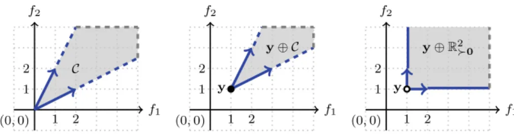
Definition 10 Minkowski Sum. The Minkowski sum (aka algebraic sum) of two setsA2Rm andB2Rmis defined as A B:¼ faþbja2A^b2Bg. Moreover we define aA¼ faaja2Ag.
f1 f2
1 1
2 2
(0,0)
C
f1 f2
1 1
2 2
(0,0)
y
y⊕ C
f1 f2
1 1
2 2
(0,0)
y
y⊕R20
Fig. 1 Example of a coneC(left), Minkowski sum of a singletonfygandC(middle), and Minkowski sum offygand the coneR2
Remark 9 For an illustration of the cone notion and examples of Minkowski sums see Fig.1.
Definition 11 The binary relation, RC, associated to the coneC. Given a coneCthe binary relation associated to this cone, notation RC, is defined as follows: 8x2Rm:8y2
Rm:ðx;yÞ 2RC if and only ify2 fxg C.
Remark 10 It is clear that for any cone C the associated binary relation is translation invariant (i.e, if 8u2Rm:ðx;yÞ 2RC ) ðxþu;yþuÞ 2RC) and also multiplication invariant by any positive real (i.e., 8a[0:ðx;yÞ 2RC ) ðax;ayÞ 2RC). Conversely, given a binary relation R which is translation invariant and multiplication invariant by any positive real, the setCR:¼
fyxj ðx;yÞ 2Rgis a cone. The above two operations are inverses of each other, i.e., to a cone C one associates a binary relationRC which is translation invariant and mul-tiplication invariant by any positive real, and the associated cone of RC is C, and conversely starting from a binary relationRwhich is translation invariant and multiplication invariant by any positive real one obtains the coneCR and
the binary relation associated to this cone isR. In short, there is a natural one to one correspondence between cones and translation invariant and multiplication-invariant-by-positive-reals binary relations onRm.
Note that for a positive multiplication invariant relation R the set CR ¼ fyxjxRyg is a cone. We restrict our
attention to relations which are translation invariant as well in order to get the above mentioned bijection between cones and relations.
Also note if a positive multiplication invariant and translation invariant relation R is such that ; 6¼R6¼RmRm, then the associated cone CR is
trivial. Relations associated to trivial cones are non-empty and not equal to all ofRmRm.
Remark 11 In general the binary relationRC associated to a cone is not reflexive nor transitive nor anti-symmetric. For instance, the binary relationRC is reflexive if and only if02 C. The following definitions are needed in order to state for which cones the associated binary relation is anti-symmetric and/or transitive.
Definition 12 Pointed cone and convex cone. A coneCis pointed if and only if C \ C f0g where C ¼ fcjc2 CgandCis convex if and only if8c12 C;c22 C;8asuch that 0a1:ac1þ ð1aÞc22 C.
With these definitions we can specify for which cones the associated relation is transitive and/or anti-symmetric:
Proposition 3 Let C be a cone and RC its associated binary relation (i.e.,RC ¼ fðx;yÞ jyx2 Cg) .Then the following statements hold.
– RC is translation and positive multiplication invariant, – RC is anti-symmetric if and only ifCis pointed, – RCis transitive if and only ifCis convex, and moreover, – RC is reflexive if and only if02 C.
A similar statement can be made if we go in the other direction, i.e.:
Proposition 4 Let R be a translation and positive multi-plication invariant binary relation and the CR the
associ-ated cone (i.e., CR ¼ fyxj ðx;yÞ 2Rg). Then the
following statements hold.
– CR is a cone,
– R is anti-symmetric if and only ifCR is pointed,
– R is transitive if and only ifCRis convex, and moreover,
– R is reflexive if and only if02 CR.
In the following definition some important subsets in Rm;m1 are introduced.
Definition 13 Letmbe a natural number bigger or equal to 1. The non-negative orthant (aka hyperoctant) of Rm, denoted by Rm
0 is the set of all elements in R
m whose
coordinates are non-negative. Furthermore, the zero-dom-inated orthant, denoted by Rm0, is the set R
m
0n f0g. Analogously we define the non-positive orthant of Rm, denoted byR0, as the set of elements inRmthe coordi-nates of which are non-positive. Furthermore, the set of elements inRmwhich dominate the zero vector0, denoted
by Rm0, is the set Rm0n f0g. The set of positive reals is denoted by R[0 and the set of non-negative reals is denoted by R0.
Remark 12 The sets defined in the previous definition are cones.
Proposition 5 The Pareto orderParetoonRmis given by
the cone order with cone Rm
0, also referred to as the
Pareto cone.
Remark 13 As Rm0 is a pointed and convex cone, the associated binary relation is irreflexive, anti-symmetric and transitive (see Proposition3). Of course, this can be veri-fied more directly.
discussion, the more general cones turned out to be very useful in generalizing the hypervolume indicator and influence the distribution of points in the approximation set to the Pareto front.
Alternatives to the standard Pareto order onRmcan be easily imagined and constructed by using pointed, convex cones. The alternatives can be used, for instance, in pref-erence articulation.
3.2 Time complexity of basic operations
on ordered sets
Partial orders do not have cycles. LetRbe a partial order. It is easy to see thatRdoes not have cycles. We show that the associated strict partial order does not have cycles. That is, there do not exist
ðb1;b2Þ 2RnD;ðb2;b3Þ 2RnD; ;ðbt1;b1Þ 2RnD
whereDis the diagonal. For suppose suchbi;i¼1; ;t
1 can be found with this property. Then by transitivity of RnD (see Proposition 1), we get ðb1;bt1Þ 2RnD. By assumption, we have ðbt1;b1Þ 2RnD. Again by transi-tivity, we getðb1;b1Þ 2RnDwhich is a contradiction. In other words,Rdoes not have cycles. (The essence of the above argument is, that any strict partial order does not have cycles.) The absence of cycles for (strict) partial orders gives rise to the following proposition.
Proposition 6 Let S be a (strict) partially ordered set. Then any finite, non-empty subset of S has minimal ele-ments (with respect to the partial order). In particular, any finite, non-empty subset YRmhas minimal elements with respect to the Pareto order Pareto. Also any, finite
non-empty subset X X has minimal elements with respect to f.
The question arises: How fast can the minimal elements be obtained?
Proposition 7 Given a finite partially ordered setðX;Þ, the set of minimal elements can be obtained in timeHðn2Þ.
Proof A double nested loop can check non-domination for each element. For the lower bound consider the case that all elements in X are incomparable. Only in this case is X the minimal set. It requires time Xðn2Þ to compare all
pairs (Daskalakis et al.2011). h
Fortunately, in case of the Pareto ordered set ðX;ParetoÞ, one can find the minimal set faster. The
algorithm suggested by Kung et al. (1975) combines a dimension sweep algorithm with a divide and conquer algorithm and finds the minimal set in timeOðnðlognÞÞfor
d¼2 and in timeOðnðlognÞd2Þford3. Hence, in case
of small finite decision spaces, efficient solutions can be identified without much effort. In the case of large com-binatorial or continuous search spaces, however, opti-mization algorithms are needed to find them.
4 Scalarization techniques
Classically, multiobjective optimization problems are often solved using scalarization techniques (see, for instance, Miettinen 2012). Also in the theory and practice of evo-lutionary multiobjective optimization scalarization plays an important role, especially in the so-called decomposition based approaches.
In brief, scalarization means that the objective functions are aggregated (or reformulated as constraints), and then a constrained single-objective problem is solved. By using different parameters of the constraints and aggregation function, it is possible to obtain different points on the Pareto front. However, when using such techniques, certain caveats have to be considered. In fact, one should always ask the following two questions:
1. Does the optimization of scalarized problems result in efficient points?
2. Can we obtain all efficient points or vectors on the Pareto front by changing the parameters of the scalarization function or constraints?
We will provide four representative examples of scalar-ization approaches and analyze whether they have these properties.
4.1 Linear weighting
A simple means to scalarize a problem is to attach non-negative weights (at least one of them positive) to each objective function and then to minimize the weighted sum of objective functions. Hence, the multiobjective opti-mization problem is reformulated to:
Definition 14 Linear Scalarization Problem. The linear scalarization problem (LSP) of an MOP using a weight vector w2Rm
0, is given by
minimize X
m
i¼1
wifiðxÞ;x2 X:
Proposition 8 The solution of an LSP is on the Pareto front, no matter which weights in Rm0 are chosen.
Proof We show that the solution of the LSP cannot be a dominated point, and therefore, if it exists, it must neces-sarily be a non-dominated point. Consider a solution of the LSP against some weights w2Rm
this minimal point is dominated. Then there exists an objective vectory2fðX Þwith8i2 f1;. . .;mg yifiðxÞ
and for some indexj2 f1;. . .;mg it holds thatyj\fjðxÞ.
Hence, it must also hold that Pmi¼1wiyi\Pmi¼1wifiðxÞ,
which contradicts the assumption thatx is minimal. h
In the literature the notion of convexity (concavity) of Pareto fronts is for the most part not defined formally. Possible formal definitions for convexity and concavity are as follows.
Definition 15 Convex Pareto front. A Pareto front is convex if and only ifYN Rm0 is convex.
Definition 16 Concave Pareto front. A Pareto front is concave if and only ifYN Rm0 is convex.
Proposition 9 In case of a convex Pareto front, for each solution inYN there is a solution of a linear scalarization
problem for some weight vector w2Rm
0.
If the Pareto front is non-convex, then, in general, there can be points on the Pareto front which are the solutions of no LSP. Practically speaking, in the case of concave Pareto fronts, the LSP will tend to give only extremal solutions, that is, solutions that are optimal in one of the objectives. This phenomenon is illustrated in Fig.2, where the tan-gential points of the dashed lines indicate the solution obtained by minimizing an LSP for different weight choi-ces (colors). In the case of the non-convex Pareto front (Fig.2, right), even equal weights (dark green) cannot lead to a solution in the middle part of the Pareto front. Also, by solving a series of LSPs with minimizing different weighted aggregation functions, it is not possible to obtain this interesting part of the Pareto front.
4.1.1 Chebychev scalarization
Another means of scalarization, that will also uncover points in concave parts of the Pareto front, is to formulate
the weighted Chebychev distance to a reference point as an objective function.
Definition 17 Chebychev Scalarization Problem. The Chebychev scalarization problem (CSP) of an MOP using a weight vector k2Rm0, is given by
minimize max
i2f1;...;mgkijfiðxÞ z
ij;x2 X;
wherezis a reference point, i.e., the ideal point defined as zi ¼infx2XfiðxÞwithi¼1; ;m.
Proposition 10 Let us assume a given set of mutually non-dominated solutions inRm(e.g., a Pareto front). Then for
every non-dominated point pthere exists a set of weights for a CSP, that makes this point a minimizer of the CSP provided the reference pointzis properly chosen(i.e., the vector pz either lies in the positive or negative orthant).
Practically speaking, Proposition 10 ensures that by changing the weights, all points of the Pareto front can, in principle, occur as minimizers of CSP. For the two example Pareto fronts, the minimizers of the Chebychev scalarization function are points on the iso-height lines of the smallest CSP function value which still intersect with the Pareto front. Clearly, such points are potentially found in convex parts of Pareto fronts as illustrated in Fig.3(left) as well as in concave parts (right).However, it is easy to construct examples where a CSP obtains minimizers in weakly dominated points (see Definition 8). Think for instance of the casefðX Þ ¼ ½0;12. In this case all points on
the line segment ð0;0Þ>;ð0;1Þ> and on the line segment
ð0;0Þ>ð1;0Þ> are solutions of some Chebychev scalariza-tion. (The ideal point is 0¼ ð0;0Þ>, one can take as weights (0, 1) for the first scalarization, and (1, 0) for the second scalarization; the Pareto front is equal tofð0;0Þ>g). In order to prevent this, the augmented Chebychev scalarization provides a solution. It reads:
f1 f2
1 1
2 2
3 3
(0,0)
y∗
y∗ y∗
f1 f2
1 1
2 2
3 3
(0,0)
y∗
y∗ y∗ Fig. 2 Linear scalarization
minimize max
i2f1;...;mgkifiðxÞ þ
Xn
i¼1
fiðxÞ;x2 X; ð2Þ
whereis a sufficiently small, positive constant.
4.1.2 -constraint method
A rather straightforward approach to turn a multiobjective optimization problem into a constraint single-objective optimization problem is the-constraint method.
Definition 18 –constraint Scalarization. Given a MOP, the–constraint scalarization is defined as follows. Given m1 constants 12R;. . .; m12R,
minimizef1ðxÞ; subject tog1ðxÞ 1;. . .;gm1ðxÞ m1;
where f1;g1;. . .;gm1 constitute the m components of vector functionf of the multiobjective optimization prob-lem (see Definition1).
The method is illustrated in Fig.4(left) for1¼2:5 for a biobjective problem. Again, by varying the constants 1 2R;. . .; m12R, one can obtain different points on the Pareto front. And again, among the solutions weakly dominated solutions may occur. It can, moreover, be
difficult to choose an appropriate range for thevalues, if there is no prior knowledge of the location of the Pareto front inRm.
4.1.3 Boundary intersection methods
Another often suggested way to find an optimizer is to search for intersection points of rays with the attained subset fðX Þ (Jaszkiewicz and Słowin´ski 1999). For this method, one needs to choose a reference point inRm, sayr, which, if possible, dominates all points in the Pareto front. Alternatively, in the Normal Boundary Intersection method (Das and Dennis1998) the rays can emanate from a line (in the bi-objective case) or anm1 dimensional hyperplane, in which case lines originate from different evenly spaced reference points (Das and Dennis1998). Then the follow-ing problem is solved:
Definition 19 Boundary Intersection Problem. Let d2 Rm
0 denote a direction vector and r2R
mdenote the
ref-erence vector. Then the boundary intersection problem is formulated as:
f1 f2
1 1
2 2
3 3
(0,0)
y∗
y∗ y∗
f1 f2
1 1
2 2
3 3
(0,0)
y∗
y∗
y∗ Fig. 3 Chebychev scalarization
problems with different weights for (1) convex Pareto fronts, and (2) concave Pareto fronts
f1 f2
1 1
2 2
3 3
(0,0)
y
∗
f1 f2
1 1
2 2
3 3
(0,0)
d y∗
r Fig. 4 Re-formulation of
minimizet;
subject to
ðaÞrþtdfðxÞ ¼0; ðbÞx2 X; and ðcÞt2R0
Constraints (a) and (b) in the above problem formulation enforce that the point is on the ray and also that there exists a pre-image of the point in the decision space. Becausetis minimized, we obtain the point that is closest to the ref-erence point in the direction ofd. This method allows some intuitive control on the position of resulting Pareto front points. Excepting rare degenerate cases, it will obtain points on the boundary of the attainable setfðX Þ. However, it also requires an approximate knowledge of the position of the Pareto front. Moreover, it might result in dominated points if the Pareto front is not convex. The method is illustrated in Fig.4 (left) for a single direction and refer-ence point.
5 Numerical algorithms
Many of the numerical algorithms for solving multiobjec-tive optimization problems make use of scalarization with varying parameters. It is then possible to use single-ob-jective numerical optimization methods for finding differ-ent points on the Pareto front.
Besides these, there are methods that focus on solving the Karush-Kuhn-Tucker conditions. These methods aim for covering all solutions to the typically underdetermined nonlinear equation system given by these condition. Again, for the sake of clarity and brevity, in the following treat-ment, we will focus on the unconstrained case, noting that the full Karush-Kuhn-Tucker and Fritz-John conditions also feature equality and inequality constraints (Kuhn and Tucker1951).
Definition 20 Local Efficient Point. A point x2 X is locally efficient, if there exists 2R[0 such that 6 9y2 BðxÞ:yf xandx6¼y, where BðxÞ denotes the
open-ball aroundx.
Theorem 1 Fritz–John Conditions. A neccessary condi-tion forx2 X to be locally efficient is given by
9k0:X
m
i¼1
kirfiðxÞ ¼0 and Xm
i¼1
ki¼1:
Theorem 2 Karush–Kuhn–Tucker Conditions. A point x2 X is locally efficient, if it satisfies the Fritz–John
conditions and for which all objective functions are convex in some open -ballBðxÞaroundx.
Remark 14 The equation in the Fritz–John Condition typically does not result in a unique solution. For an n -dimensional decision spaceXwe havenþ1 equations and we have mþn unknowns (including the k multipliers). Hence, in a non-degenerate case, the solution set is of dimensionm1.
It is possible to use continuation and homotopy methods to obtain all the solutions. The main idea ofcontinuation methodsis to find a single solution of the equation system and then to expand the solution set in the neighborhood of this solution. To decide in which direction to expand, it is necessary to maintain an archive, sayA, of points that have already been obtained. To obtain a new point xnew in the
neighborhood of a given point from the archivex2Athe homotopy method conducts the following steps:
1. Using the implicit function theorem a tangent space at the current point is obtained. It yielded an m1 dimensional hyperplane that is tangential to fðxÞ and used to obtain a predictor. See for the implicit function theorem, for instance, Krantz and Parks (2003). 2. A point on the hyperplane in the desired direction is
obtained, thereby avoiding regions that are already well covered inA.
3. A corrector is computed minimizing the residual jjPkifiðxÞjj.
4. In case the corrector method succeeded to obtain a new point in the desired neighborhood, the new point is added to the archive. Otherwise, the direction is saved (to avoid trying it a second time).
See Hillermeier (2001) and Schu¨tze et al. (2005) for examples and more detailed descriptions. The continuation and homotopy methods require the efficient set to be connected. Moreover, they require points to satisfy certain regularity conditions (local convexity and differentiability). Global multiobjective optimization research is still a very active field of research. There are some promising directions, such as subdivision techniques (Dellnitz et al.
2005), Bayesian global optimization (Emmerich et al.
2016), and Lipschitz optimization (Zˇ ilinskas2013). How-ever, these require the decision space to be of low dimension.
6 Evolutionary multiobjective optimization
Evolutionary algorithms are a major branch of bio-inspired search heuristics, which originated in the 1960ties and are widely applied to solve combinatorial and non-convex numerical optimization problems. In short, they use para-digms from natural evolution, such as selection, recombi-nation, and mutation to steer a population (set) of individuals (decision vectors) towards optimal or near-op-timal solutions (Ba¨ck1996).
Multiobjective evolutionary algorithms (MOEAs) gen-eralize this idea, and typically they are designed to grad-ually approach sets of Pareto optimal solutions that are well-distributed across the Pareto front. As there are—in general—no single-best solutions in multiobjective opti-mization, the selection schemes of such algorithms differ from those used in single-objective optimization. First MOEAs were developed in the 1990ties—see, e.g., Kur-sawe (1990) and Fonseca and Fleming (1993), but since around the year 2001, after the first book devoted exclu-sively to this topic was published by Deb (2001), the number of methods and results in this field grew rapidly.
With some exceptions, the distinction between different classes of evolutionary multiobjective optimization algo-rithms is mainly due to the differences in the paradigms used to define the selection operators, whereas the choice of the variation operators is generic and dependent on the problem. As an example, one might consider NSGA-II (see Deb et al.2002) as a typical evolutionary multiobjective optimization algorithm; NSGA-II can be applied to con-tinuous search spaces as well as to combinatorial search
spaces. Whereas the selection operators stay the same, the variation operators (mutation, recombination) must be adapted to the representations of solutions in the decision space.
There are currently three main paradigms for MOEA designs. These are:
1. Pareto based MOEAs: The Pareto based MOEAs use a two-level ranking scheme. The Pareto dominance relation governs the first ranking and contributions of points to diversity is the principle of the second level ranking. The second level ranking applies to points that share the same position in the first ranking. NSGA-II (see Deb et al. 2002) and SPEA2 (see Zitzler and Thiele1999) are two popular algorithms that fall into this category.
2. Indicator based MOEAs: These MOEAs are guided by an indicator that measures the performance of a set, for instance, the hypervolume indicator or the R2 indica-tor. The MOEAs are designed in a way that improve-ments concerning this indicator determine the selection procedure or the ranking of individuals.
3. Decomposition based MOEAs: Here, the algorithm decomposes the problem into several subproblems, each one of them targeting different parts of the Pareto front. For each subproblem, a different parametrization (or weighting) of a scalarization method is used. MOEA/D and NSGA-III are well-known methods in this domain.
In this tutorial, we will introduce typical algorithms for each of these paradigms: NSGA-II, SMS-EMOA, and
Algorithm 1NSGA-II Algorithm 1: initialize populationP0⊂ Xµ
2: whilenot terminatedo 3: {Begin variate} 4: Qt← ∅
5: for alli∈ {1, . . . , μ}do
6: (x(1),x(2))←select mates(Pt){select two parent individualsx(1)∈Ptandx(2)∈
Pt}
7: r(ti)←recombine(x(1),x(2))
8: q(ti)←mutate(r)
9: Qt←Qt∪ {q(ti)} 10: end for
11: {End variate}
12: {Selection step, selectμ-”best” out of (Pt∪Qt) by a two step procedure:} 13: (R1, ..., R)← non-dom sort(f, Pt∪Qt)
14: Find the element of the partition,Riµ, for which the sum of the cardinalities|R1|+
· · ·+|Riµ|is for the first time≥μ. If|R1|+· · ·+|Riµ|=μ,Pt+1← ∪iiµ=1Ri, otherwise determine setHcontainingμ−(|R1|+· · ·+|Riµ−1|) elements fromRiµ with the
highest crowding distance andPt+1←(∪iiµ=1−1Ri)∪H. 15: {End of selection step.}
MOEA/D. We will discuss important design choices, and how and why other, similar algorithms deviate in these choices.
6.1 Pareto based algorithms: NSGA-II
The basic loop of NSGA-II (Deb et al.2002) is given by Algorithm 1.
Firstly, a population of points is initialized. Then the followinggenerational loopis repeated. This loop consists of two parts. In the first, the population undergoes a vari-ation. In the second part, a selection takes place which results in the new generation-population. The generational loop repeats until it meets some termination criterion, which could be convergence detection criterion (cf. Wag-ner et al.2009) or the exceedance of a maximal compu-tational budget.
In the variation part of the loopk offspring are gener-ated. For each offspring, two parents are selected. Each one of them is selected using binary tournament selection, that is drawing randomly two individuals fromPtand selecting
the better one concerning its rank in the population. The parents are then recombined using a standard recombina-tion operator. For real-valued problems simulated binary crossover (SBX) is used (see Deb and Argawal 1995). Then the resulting individual is mutated. For real-valued problem polynomial mutation (PM) is used (see Mateo and Alberto2012). This way, kindividuals are created, which are all combinations or modifications of individuals inPt.
Then the parent and the offspring populations are merged intoPt[Qt.
In the second part, the selection part, thel best indi-viduals ofPt[Qtwith respect to a multiobjective ranking
are selected as the new populationPtþ1.
Next we digress in order to explain the multiobjective ranking which is used in NSGA-II. The key ingredient of NSGA-II that distinguishes it from genetic algorithms for single-objective optimization, is the way the individuals are ranked. Theranking procedure of NSGA-IIconsists of
two levels. First, non-dominated sorting is performed. This ranking solely depends on the Pareto order and does not depend on diversity. Secondly, individuals which share the same rank after the first ranking are then ranked according to the crowding distance criterion which is a strong reflection of the diversity.
Let NDðPÞdenote the non-dominated solutions in some population. Non-dominated sorting partitions the popula-tions into subsets (layers) based on Pareto non-dominance and it can be specified through recursion as follows.
R1¼NDðPÞ ð3Þ
Rkþ1¼NDðPn [ki¼1RiÞ;k¼1;2;. . . ð4Þ
As in each step of the recursion at least one solution is removed from the population, the maximal number of layers is |P|. We will use the index‘to denote the highest non-empty layer. The rank of the solution after non-dom-inated sorting is given by the subindexkof Rk. It is clear
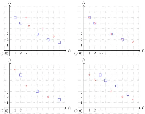
that solutions in the same layer are mutually incomparable. The non-dominated sorting procedure is illustrated in Fig.5 (upper left). The solutions are ranked as follows R1 ¼ fyð1Þ;yð2Þ;yð3Þ;yð4Þg, R2¼ fyð5Þ;yð6Þ;yð7Þg, R3¼ fyð8Þ;yð9Þg.
Now, if there is more than one solution in a layer, sayR, a secondary ranking procedure is used to rank solutions within that layer. This procedure applies the crowding distance criterion. The crowding distance of a solutionx2 R is computed by a sum over contributions ci of thei-th
objective function:
liðxÞ:¼maxðffiðyÞjy2Rn fxg ^fiðyÞ fiðxÞg [ f1gÞ
ð5Þ
uiðxÞ:¼minðffiðyÞjy2Rn fxg ^fiðyÞ fiðxÞg [ f1gÞ
ð6Þ
ciðxÞ:¼uili; i¼1;. . .;m ð7Þ
The crowding distance is now given as: f
f2
1 1
2 2
3 3
(0,0)
y(1)
y(2)
y(3)
y(4)
y(5) y(6)
y(7) y(8) y(9)
1 f1
f2
1 1
2 2
3 3
(0,0)
y(1)
y(2) y(3)
y(4)
y(5) Fig. 5 Illustration of
cðxÞ:¼1 m
Xm
i¼1
ciðxÞ;x2R ð8Þ
Form¼2 the crowding distances of a set of mutually non-dominated points are illustrated in Fig.5(upper right). In this particular case, they are proportional to the perimeter of a rectangle that just is intersecting with the neighboring points (up to a factor of 1
4). Practically speaking, the value of li is determined by the nearest
neighbor ofxto the leftaccording to the i-coordinate, and li is equal to the i-th coordinate of this nearest neighbor,
similarly the value of ui is determined by the nearest
neighbor of x to the right according to the i-coordinate, andui is equal to thei-th coordinate of this right nearest
neighbor. The more space there is around a solution, the higher is the crowding distance. Therefore, solutions with a high crowding distance should be ranked better than those with a low crowding distance in order to maintain diversity in the population. This way we establish a second order ranking. If the crowding distance is the same for two points, then it is randomly decided which point is ranked higher.
Now we explain the non-dom_sort procedure in line 13 of Algorithm 1 the role ofP is taken over byPt\Qt: In
order to select thelbest members ofPt[Qtaccording to
the above described two level ranking, we proceed as follows. Create the partition R1;R2; ;R‘ of Pt[Qt as
described above. For this partition one finds the first index ilfor which the sum of the cardinalitiesjR1j þ þ jRiljis
for the first time l. If jR1j þ þ jRilj ¼l, then set
Ptþ1 to [
il
i¼1Ri, otherwise determine the set Hcontaining
l ðjR1j þ þ jRil1jÞ elements from Ril with the
highest crowding distance and set the next
generation-population,Ptþ1, toð[
il1
i¼1 RiÞ [H.
Pareto-based Algorithms are probably the largest class of MOEAs. They have in common that they combine a ranking criterion based on Pareto dominance with a diversity based secondary ranking. Other common algo-rithms that belong to this class are as follows. The Mul-tiobjective Genetic Algorithm (MOGA) (Fonseca and Fleming 1993), which was one of the first MOEAs. The PAES (Knowles and Corne2000), which uses a grid par-titioning of the objective space in order to make sure that certain regions of the objective space do not get too crowded. Within a single grid cell, only one solution is selected. The Strength Pareto Evolutionary Algorithm (SPEA) (Zitzler and Thiele1999) uses a different criterion for ranking based on Pareto dominance. The strength of an
individual depends on how many other individuals it dominates and by how many other individuals dominate it. Moreover, clustering serves as a secondary ranking crite-rion. Both operators have been refined in SPEA2 (Zitzler et al. 2001), and also it features a strategy to maintain an archive of non-dominated solutions. The Multiobjective Micro GA.
Coello and Pulido (2001) is an algorithm that uses a very small population size in conjunction with an archive. Finally, the Differential Evolution Multiobjective Opti-mization (DEMO) (Robic and Filipic 2005) algorithm combines concepts from Pareto-based MOEAs with a variation operator from differential evolution, which leads to improved efficiency and more precise results in partic-ular for continuous problems.
6.2 Indicator-based algorithms: SMS-EMOA
A second algorithm that we will discuss is a classical algorithm following the paradigm of indicator-based mul-tiobjective optimization. In the context of MOEAs, by a performance indicator (or just indicator), we denote a scalar measure of the quality of a Pareto front approxi-mation. Indicators can beunary, meaning that they yield an absolute measure of the quality of a Pareto front approxi-mation. They are called binary, whenever they measure how much better one Pareto front approximation is con-cerning another Pareto front approximation.
The SMS-EMOA (Emmerich et al. 2005) uses the hypervolume indicator as a performance indicator. Theo-retical analysis attests that this indicator has some favor-able properties, as the maximization of it yields approximations of the Pareto front with points located on the Pareto front and well distributed across the Pareto front. The hypervolume indicator measures the size of the dom-inated space, bound from above by a reference point.
For an approximation set ARm it is defined as
follows:
HIðAÞ ¼Volðfy2Rm:yParetor^ 9a2A :aParetoygÞ ð9Þ
the dominated space is infinite, it is necessary to bound it. For this reason, the reference pointris introduced.
The SMS-EMOA seeks to maximize the hypervolume indicator of a population which serves as an approximation set. This is achieved by considering the contribution of points to the hypervolume indicator in the selection pro-cedure. Algorithm 2 describes the basic loop of the stan-dard implementation of the SMS-EMOA.
The algorithm starts with the initialization of a popula-tion in the search space. Then it creates onlyoneoffspring individual by recombination and mutation. This new indi-vidual enters the population, which has now sizelþ1. To reduce the population size again to the size ofl, a subset of sizelwith maximal hypervolume is selected. This way as long as the reference point for computing the hypervolume
remains unchanged, the hypervolume indicator of Pt can
only grow or stay equal with an increasing number of iterationst.
Next, the details of the selection procedure will be dis-cussed. If all solutions in Pt are non-dominated, the
selection of a subset of maximal hypervolume is equivalent to deleting the point with the smallest (exclusive) hyper-volume contribution. The hyperhyper-volume contribution is defined as:
DHIðy;YÞ ¼HIðYÞ HIðYn fygÞ
An illustration of the hypervolume indicator and hypervolume contributions for m¼2 and, respectively, m¼3 is given in Fig.6. Efficient computation of all hypervolume contributions of a population can be achieved
Algorithm 2SMS-EMOA initializeP0⊂ Xµ
whilenot terminatedo {Begin variate}
(x(1),x(2))←select mates(Pt){select two parent individualsx(1)∈Ptandx(2)∈Pt}
ct←recombine(x(1),x(2)) qt←mutate(ct)
{End variate} {Begin selection}
Pt+1←selectf(Pt∪{qt}){Select subset of sizeμwith maximal hypervolume indicator fromP∪ {qt}}
{End selection} t←t+ 1 end while return Pt
f1 f1
f2
1 1
2 2
3 3
(0,0)
y(1)
y(2)
y(3)
y(4)
y(5) r
Y ⊕R20
f2
1 1
2 2
3 3
(0,0)
y(1)
y(2)
y(3)
y(4)
y(5) r
f3
f1 f2
y(1) y(2)
y(3) y(4)
y(5)
f3
f1 f2
y(1) y(2)
y(3) y(4)
y(5) Fig. 6 Illustration of 2-D
in timeHðlloglÞ for m¼2 and m¼3 (Emmerich and Fonseca 2011). Form¼3 or 4, fast implementations are described in Guerreiro and Fonseca (2017). Moreover, for fast logarithmic-time incremental updates for 2-D an algorithm is described in Hupkens and Emmerich (2013). For achieving logarithmic time updates in SMS-EMOA, the non-dominated sorting procedure was replaced by a procedure, that sorts dominated solutions based on age. For m[2, fast incremental updates of the hypervolume indi-cator and its contributions were proposed in for more than two dimensions (Guerreiro and Fonseca2017).
In case dominated solutions appear the standard imple-mentation of SMS-EMOA partitions the population into layers of equal dominance ranks, just like in NSGA-II. Subsequently, the solution with the smallest hypervolume contribution on the worst ranked layer gets discarded.
SMS-EMOA typically converges to regularly spaced Pareto front approximations. The density of these approx-imations depends on the local curvature of the Pareto front. For biobjective problems, it is highest at points where the slope is equal to45(Auger et al.2009). It is possible to influence the distribution of the points in the approximation set by using a generalized cone-based hypervolume indi-cator. These indicators measure the hypervolume domi-nated by a cone-order of a given cone, and the resulting optimal distribution gets more uniform if the cones are acute, and more concentrated when using obtuse cones (see Emmerich et al.2013).
Besides the SMS-EMOA, there are various other indi-cator-based MOEAs. Some of them also use the hyper-volume indicator. The original idea to use the hyperhyper-volume indicator in an MOEA was proposed in the context of archiving methods for non-dominated points. Here the hypervolume indicator was used for keeping a bounded-size archive (Knowles et al. 2003). Besides, in an early work hypervolume-based selection which also introduced a novel mutation scheme, which was the focus of the paper (Huband et al. 2003). The term Indicator-based Evolu-tionary Algorithms (IBEA) (Zitzler and Ku¨nzli2004) was introduced in a paper that proposed an algorithm design, in which the choice of indicators is generic. The hypervol-ume-based IBEA was discussed as one instance of this class. Its design is however different to SMS-EMOA and makes no specific use of the characteristics of the hyper-volume indicator. The Hyperhyper-volume Estimation Algorithm (HypE) (Bader and Zitzler 2011) uses a Monte Carlo Estimation for the hypervolume in high dimensions and thus it can be used for optimization with a high number of objectives (so-called many-objective optimization prob-lems). MO-CMA-ES (Igel et al. 2006) is another hyper-volume-based MOEA. It uses the covariance-matrix adaptation in its mutation operator, which enables it to adapt its mutation distribution to the local curvature and
scaling of the objective functions. Although the hypervol-ume indicator has been very prominent in IBEAs, there are some algorithms using other indicators, notably this is the R2 indicator (Trautmann et al. 2013), which features an ideal point as a reference point, and the averaged Hausdorff distance (Dp indicator) (Rudolph et al. 2016), which requires an aspiration set or estimation of the Pareto front which is dynamically updated and used as a reference. The idea of aspiration sets for indicators that require knowledge of the ‘true’ Pareto front also occurred in conjunction with thea-indicator (Wagner et al.2015), which generalizes the approximation ratio in numerical single-objective opti-mization. The Portfolio Selection Multiobjective Opti-mization Algorithm (POSEA) (Yevseyeva et al.2014) uses the Sharpe Index from financial portfolio theory as an indicator, which applies the hypervolume indicator of singletons as a utility function and a definition of the covariances based on their overlap. The Sharpe index combines the cumulated performance of single individuals with the covariance information (related to diversity), and it has interesting theoretical properties.
6.3 Decomposition-based algorithm: MOEA/D
Decomposition-based algorithms divide the problem into subproblems using scalarizations based on different weights. Each scalarization defines a subproblem. The subproblems are then solved simultaneously by dynami-cally assigning and re-assigning points to subproblems and exchanging information from solutions to neighboring sub-problems.
The method defines neighborhoods on the set of these subproblems based on the distances between their aggre-gation coefficient vectors. When optimizing a subproblem, information from neighboring subproblems can be exchanged, thereby increasing the efficiency of the search as compared to methods that independently solve the subproblems.
MOEA/D (Zhang and Li2007) is a very commonly used decomposition based method, that succeeded a couple of preceding algorithms based on the idea of combining decomposition, scalarization and local search(Ishibuchi and Murata1996; Jin et al.2001; Jaszkiewicz2002). Note that even the early proposed algorithms VEGA (Schaffer
D one population with interacting neighboring individuals is applied, which reduces the complexity of the algorithm. Typically, MOEA/D works with Chebychev scalariza-tions, but the authors also suggest other scalarization methods, namely scalarization based on linear weighting— which however has problems with approximating non-convex Pareto fronts—and scalarization based on boundary intersection methods—which requires additional parame-ters and might also obtain strictly dominated points.
MOEA/D evolves a population of individuals, each individualxðiÞ2P
t being associated with a weight vector
kðiÞ. The weight vectors kðiÞ are evenly distributed in the search space, e.g., for two objectives a possible choice is: kðiÞ¼ ðki
k ; i kÞ
>;i ¼ 0;. . .; l.
The i-th subproblem gðxjki;zÞis defined by the Che-bychev scalarization function (see also Eq.2):
gðxjkðiÞ;zÞ ¼ max
j2f1;...;mgfk ðiÞ
j jfjðxÞ zjjg þ Xm
j¼1
fjðxÞ zj
ð10Þ
The main idea is that in the creation of a new candidate solution for the i-th individual the neighbors of this indi-vidual are considered. A neighbor is an incumbent solution
of a subproblem with similar weight vectors. The neigh-borhood ofi-th individual is the set ofksubproblems, for
so predefined constant k, that is closest to kðiÞ in the Euclidean distance, including thei-th subproblem itself. It
is denoted withB(i). Given these preliminaries, the MOEA/ D algorithm—using Chebychev scalarization— reads as described in Algorithm 3.
Note the following two remarks about MOEA/D: (1) Many parts of the algorithm are kept generic. Here, generic options are recombination, typically instantiated by stan-dard recombination operators from genetic algorithms, and local improvement heuristic. The local improvement heuristic should find a solution in the vicinity of a given solution that does not violate constraints and has a rela-tively good performance concerning the objective function values. (2) MOEA/D has additional statements to collect all non-dominated solutions it generates during a run in an external archive. Because this external archive is only used in the final output and does not influence the search dynamics, it can be seen as a generic feature of the algo-rithm. In principle, an external archive can be used in all EMOAs and could therefore also be done in SMS-EMOA and NSGA-II. To make comparisons to NSGA-II and SMS-EMOA easier, we omitted the archiving strategy in the description.
Recently, decomposition-based MOEAs became very popular, also because they scale well to problems with many objective functions. The NSGA-III (Deb and Jain
2014) algorithm is specially designed for many-objective optimization and uses a set of reference points that is dynamically updated in its decomposition. Another
decomposition based technique is called Generalized Decomposition (Giagkiozis et al. 2014). It uses a mathe-matical programming solver to compute updates, and it was shown to perform well on continuous problems. The combination of mathematical programming and decom-position techniques is also explored in other, more novel, hybrid techniques, such as Directed Search (Schu¨tze et al.
Algorithm 3MOEA/D
input:Λ={λ(1), ..., λ(µ)} {weight vectors} input:z∗: reference point for Chebychev distance initializeP0⊂ Xµ
initialize neighborhoodsB(i) by collectingknearest weight vectors inΛfor eachλ(i)
whilenot terminatedo for alli∈ {1, ..., μ}do
Select randomly two solutionsx(1),x(2)in the neighborhoodB(i). y←Recombinex(1),x(2)by a problem specific recombination operator.
y ←Local problem specific, heuristic improvement ofy, e.g. local search, based on the scalarized objective functiong(x|λ(i),z∗) .
if g(y|λ(i),z∗)< g(x(i)|λ(i),z∗)then x(i)←y
end if
Update z∗, if neccessary, i.e, one of its component is larger than one of the corre-sponding components off(x(i)).
end for
2016), which utilizes the Jacobian matrix of the vector-valued objective function (or approximations to it) to find promising directions in the search space, based on desired directions in the objective space.
7 Performance assessment
In order to make a judgement (that is, gain insight into the advantages and disadvantages) of multiobjective evolu-tionary (or for that matter also deterministic) optimizers we need to take into account (1) the computational resources used, and (2) the quality of the produced result(s).
The current state of the art of multiobjective optimiza-tion approaches are mainly compared empirically though theoretical analyses exist (see, for instance, the conver-gence results described in Rudolph and Agapie (2000), Beume et al. (2011) albeit for rather simple problems as more realistic problems elude mathematical analysis.
The most commonly computational resource which is taken into account is the computation time which is very often measured implicitly by counting fitness function evaluations—in this respect, there is no difference with single-objective optimization. In contrast to single-objec-tive optimization, in multiobjecsingle-objec-tive optimization, a close distance to a (Pareto) optimal solution is not the only thing required but also good coverage of the entire Pareto front. As the results of multiobjective optimization algorithms are (finite) approximation sets to the Pareto front we need to be able to say when one Pareto front approximation is better than another. One good way to define when one approxi-mation set is better than another is as in Definition22(see Zitzler et al.2003).
Definition 21 Approximation Set of a Pareto Front. A finite subsetA of Rm is an approximation set of a Pareto front if and only if A consists of mutually (Pareto) non-dominated points.
Definition 22 Comparing Approximation Sets of a Pareto Front. LetAand Bbe approximation sets of a Pareto front
inRm. We say thatA is better thanBif and only if every
b2Bis weakly dominated by at least one element a2A andA6¼B. Notation:A.B.
In Fig.7examples are given of the case of one set being better than another and in Fig.8examples are given of the case that a set is not better than another.
This relation on sets has been used in Zitzler et al. (2003) to classify performance indicators for Pareto fronts. To do so, they introduced the notion of completeness and compatibility of these indicators with respect to the set relation ‘is better than’.
Definition 23 Unary Set Indicator. A unary set indicator is a mapping from finite subsets of the objective space to the set of real numbers. It is used to compare (finite) approx-imations to the Pareto front.
Definition 24 Compatibility of Unary Set Indicators concerning the ‘is better than’ order on Approximation Sets. A unary set indicator Iis compatible concerning the ‘is better than’ or .-relation if and only if IðAÞ[IðBÞ )A.B. A unary set indicator I is complete with respect to the ‘is better than’ or.-relation if and only ifA.B)IðAÞ[IðBÞ. If in the last definition we replace[
by then the indicator is called weakly-complete.
The hypervolume indicator and some of its variations are complete. Other indicators compared in the paper (Zitzler et al. 2003) are weakly-complete or not even weakly-complete. It has been proven in the same paper that no unary indicator exists that is complete and compatible at the same time. Moreover for the hypervolume indicator HI it has be shown that HIðAÞ[ HIðBÞ ) :ðB.AÞ. The latter we call weakly-compatible.
In all the discussions of the hypervolume indicator, the assumption is that all points of the approximation sets under consideration dominate the reference point. Recently, variations of the hypervolume indicator have been proposed—the so-called free hypervolume indica-tors—that do not require the definition of a reference point
f1 f2
1 1
2 2
. . .
. . .
(0,0)
◦ ◦
◦
◦
f1 f2
1 1
2 2
. . .
. . .
(0,0)
◦ ◦
◦
◦ Fig. 7 In the left picture, the set
and are complete and weakly-compatible for all approxi-mation sets (Zitzler et al.2003).
Besides unary indicators, one has introduced binary indicators (see Riquelme et al.2015). The most used ones are unary indicators followed up by binary indicators. For binary indicators, the input is a pair of approximation sets and the output is again a real number. Here the goal is to determine which of the two approximation sets is the better one (and how much better it is)1. Binary indicators can also be used, if the true Pareto front is known, e.g., in bench-marking on test problems. A common binary indicator is the binary-indicator. In order to introduce this indicator we first define for each d2R a binary relation on the points inRm.
Definition 25 d-domination. Let d2R and let a2Rm and b2Rm. We say that a d-dominates b (notation: adb) if and only ifaibiþd;i¼1;. . .;m.
Next, we can define the binary indicatorI.
Definition 26 The Binary Indicator I. Given two
approximation sets A and B, then
IðA;BÞ:¼infd2Rf8b2B9a2Asuch thatad bg.
Clearly for a fixedBthe smallerIðA;BÞis the better the
approximation set A is relative to B. The following
properties hold: A.B)IðB;AÞ[0, the second
notable property is as follows:
IðA;BÞ 0 andIðB;AÞ[0)A.B. These two
proper-ties show that based on the binary-indicator it is possible to decide whether or notAis better thanB. In contrast, the knowledge of the hypervolume indicator on the setsAand Bdoes not allow to decide whether or not Ais better than B.
Some of indicators are useful in case there is knowledge or complete knowledge about the Pareto front. For instance (see Rudolph et al.2016), it has been suggested to compute the Hausdorff distance (or variations of it) of an approxi-mation set to the Pareto front. Moreover, the binary -indicator can be transformed into a complete unary indi-cator in case the second input is the known Pareto front— note that this indicator needs to be minimized.
Another useful way to learn about the behavior of evolutionary multiobjective algorithms is the attainment curve approach (see da Fonseca et al.2001). The idea is to generalize the cumulative distribution function and for the study of algorithms it is approximated empirically. The distribution is defined on the set of (finite) approximation sets of the Pareto front. For each point in the objective space Rm it is the probability that the Pareto front approximation attains this point (that is, it is either one point in the approximation set, or it is dominated by some point in the approximation set). Formally, it reads
f1 f2
1 1
2 2
. . .
. . .
(0,0)
◦
◦ ◦
◦
f1 f2
1 1
2 2
. . .
. . .
(0,0) ◦
◦
◦ ◦
◦
f1 f2
1 1
2 2
. . .
. . .
(0,0) ◦
◦
◦
f1 f2
1 1
2 2
. . .
. . .
(0,0) ◦
◦
◦ ◦
◦ Fig. 8 In each of the pictures,
the set consisting of the blue square points isnotbetter than the set consisting of the red circle points. Clearly, in each of the two pictures on the right the set consisting of the red circle points is better than the set consisting of the blue square points
1 Conceivably one can can introduce k-ary indicators. To our
Pðað1Þz_að2Þz_. . ._aðkÞzÞ;
whereA¼ fað1Þ;að2Þ;. . .;aðkÞgis the approximation set and z2Rm. In other wordsPis the probability of an algorithm to find at least one solution which attains the goalz in a single run. We define the attainment functionaA:Rm!
½0;1associated to the approximation setAas follows:
aAðzÞ:¼Pðað1Þz_að2Þz_. . ._aðkÞzÞ:
This function can be approximated by
asðzÞ:¼
1 s
Xs
i¼1
I ðAi;zÞ;
whereA1;. . .;As are the outcome approximation sets of an
algorithm in s runs of the algorithm and I : ðset of approximation setsÞ Rm! f0;1g is a func-tion which associates to an approximafunc-tion set and a vector inRm the value 1 in case the vector is a member of the
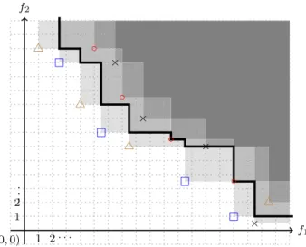
approximation set or if some element of the approximation set dominates it, otherwise the value is 0. Form¼2 or 3 we can plot the boundaries where this function changes its value. These are the attainment curves (m¼2Þ and attainment surfaces (m¼3). In particular the median attainment curve/surface gives a good summary of the behavior of the optimizer. It is the boundary where the function changes from a level below 0.5 to a level higher than 0.5. Alternatively one can look at lower and higher
levels than 0.5 in order to get an optimistic or respectively a pessimistic assessment of the performance.
In Fig.9 an example of the median attainment curve is shown. We assume that the four approximation sets are provided by some algorithm.
8 Recent topics in multiobjective
optimization
Recently, there are many new developments in the field of multiobjective optimization. Next we will list some of the most important trends.
8.1 Many-objective optimization
Optimization with more than 3 objectives is currently ter-med many-objective optimization [see, for instance, the survey (Li et al.2015)]. This is to stress the challenges one meets when dealing with more than 3 objectives. The main reasons are:
1. problems with many objectives have a Pareto front which cannot be visualized in conventional 2D or 3D plots instead other approaches to deal with this are needed;
2. the computation time for many indicators and selection schemes become computationally hard, for instance, time complexity of the hypervolume indicator compu-tation grows super-polynomially with the number of objectives, under the assumption thatP6¼NP; 3. last but not least the ratio of non-dominated points
tends to increase rapidly with the number of objectives. For instance, the probability that a point is non-dominated in a uniformly distributed set of sample points grows exponentially fast towards 1 with the number of objectives.
In the field of many-objective optimization different tech-niques are used to deal with these challenges. For the first challenge, various visualization techniques are used such as projection to lower dimensional spaces or parallel coordi-nate diagrams. In practice, one can, if the dimension is only slightly bigger than 3, express the coordinate values by colors and shape in 3D plots.
Naturally, in many-objective optimization indicators which scale well with the number of objectives (say polynomially) are very much desired. Moreover, decom-position based approaches are typically preferred to indi-cator based approaches.
The last problem requires, however, more radical devi-ations from standard approaches. In many cases, the reduction of the search space achieved by reducing it to the efficient set is not sufficiently adequate to allow for f1
f2
1 1
2 2
. . .
. . .
(0,0)
◦
◦
◦
◦
×
×
×
×