EFFICIENT TOPOLOGY MANAGEMENT AND GEOGRAPHIC ROUTING IN HIGH-CAPACITY CONTINENTAL-SCALE AIRBORNE NETWORKS
Benjamin D. Newton
A dissertation submitted to the faculty of the University of North Carolina at Chapel Hill in partial fulfillment of the requirements for the degree of Doctor of Philosophy
in the Department of Computer Science.
Chapel Hill 2017
ABSTRACT
Benjamin D. Newton: Efficient Topology Management and Geographic Routing in High-Capacity Continental-Scale Airborne Networks
(Under the direction of Kevin Jeffay and Jay Aikat)
Large-scale high-capacity communication networks among mobile airborne platforms are quickly be-coming a reality. Today, both Google and Facebook are seeking to form networks among high-flying bal-loons and drones in an effort to provide Internet connections from the stratosphere to users on the ground. This dissertation proposes an alternative, namely using the cargo and passenger aircraft already in the skies as the principal components of such a network. My work presents the design of a network architecture to overcome the challenges of managing the topology of and routing data within these continental-scale highly-dynamic networks.
The architecture relies on directional communication links, such as free-space optical communication links (FSO), to achieve high data rates over long distances. However, these state-of-the-art communication systems present new networking challenges. One such challenge is that of managing the physical topology of the network. Such a topology must be explicitly managed, ensuring that each directional data link is pointed at and connected with an appropriate neighbor (which is also pointing back) to yield an acceptable global topology. To overcome this challenge, a distributed topology management framework and associated topology generation algorithms were designed, implemented, and tested via simulation. The framework is capable of managing the topology of thousands of nodes in a continental-scale airborne network and has no communication overhead except that required to exchange position information among nearby nodes.
A second component of the work concerns routing data at high data rates through a constantly chang-ing network topology. To address this issue Topology Aware Geographic Routchang-ing (TAG), a position-based routing protocol was developed that strategically uses local topology information to make better local for-warding decisions, decreasing the number of hops required to deliver a packet, when compared with other geographic routing protocols. In addition, unlike other similar protocols, TAG is able to reliably deliver packets even when the topology changes while the packet is in flight.
To my sweetheart Erin, without whom this work would not have been possible,
ACKNOWLEDGEMENTS
It is impossible for me to appropriately express my gratitude to the numerous individuals who have made this work possible, but I will endeavor to list here some of the people who have made this work possible.
In academia, there exists an academic family tree where Ph.D. recipients can trace their academic roots. One can search for their adviser and be presented with a line of academic forefathers stretching back in time. Unlike most Ph.D. students, it has been my pleasure to have two academic ”parents” who have guided my dissertation research: Kevin Jeffay and Jay Aikat. Kevin served as my adviser and Jay as my co-adviser. Though it took some convincing initially, Kevin has always supported my cutting-edge research that is, as he says, on the “lunatic fringe”. Kevin helped me not get too lost in the “weeds” of my research and consistently gave great advice about how to proceed at each step of the process. His expert advice and wisdom guided and shaped every aspect of my research.
Jay, having herself graduated as one of Kevin’s students, was able to bridge the gap between student and adviser. She attended almost every weekly research meetings and provided needed insights, encouragement, and support for my research. Though Kevin was appointed as the department chair, and Jay accepted a top position at RENCI while serving as my advisers, they both always gave the highest priority to my needs even though they had many other important duties.
The other members of my dissertation committee include: Jasleen Kaur, Ketan Mayer-Patel and Ron Alterovitz. As I met with each of them over the course of my research they gave me ideas and suggestions that shaped and improved my research. Thank you to each of them for their service and support. Thank you to all the staff of the Computer Science department, especially Murray Anderegg, John Sopko, and Missy Wood, for their help and support. Thank you also to Gary Bishop and Fred Brooks with whom I had the privilege of meeting regularly in a Bible study group. These weekly doses of wisdom, wit, and worship are among the highlights of my time in Chapel Hill.
prediction capabilities of Tracktable, an open source software library for processing and analyzing trajectory data that has become an integral part of my dissertation research.
I am grateful for my wife’s sister Amelia Robinson for her expert editing advice, and for my wife’s parents, Brion and Deborah Robinson, for their continued support of me, my family, and our dreams. Among many other things, they sacrificed frequent-flyer miles to enable regular visits, and drove across the continent more than once. They even watched our kids for several days so my wife and I could attend a conference. Thank you to them for their continued support.
It is hard to express the gratitude I feel for my parents Dave and Sandy Newton. They raised an inquisi-tive boy and have shaped and molded him into a scholar. Without their continued support, this work would not have been possible. Thank you, Mom and Dad, for the packages from home, for your regular visits, and for your generous gifts! Thank you also, to my sister, Stacy Schultz, and her husband Brian for always believing in me.
My children have given up many evenings and Saturday afternoons when they wish they could have been with Dad. Thank you to my 11-year-old Libby, for helping find acronyms in my manuscript and for her interest and support of my research. Thank you to my 6-year-old Emma for squealing “Daddy” and running to give me a hug upon my arrival at home. And thank you to my 1-year-old Samuel, who always tried to help write my dissertation by typing on the keyboard whenever I set my laptop down.
TABLE OF CONTENTS
LIST OF TABLES . . . xiv
LIST OF FIGURES . . . xv
LIST OF ABBREVIATIONS . . . xx
1 CHAPTER 1: INTRODUCTION . . . 1
1.1 Airborne Networks of Balloons, Drones, and Commercial Aircraft . . . 1
1.2 Free-Space Optical Communication Links . . . 3
1.3 Distributed Explicit Topology Management . . . 4
1.4 Routing in Large-Scale Airborne Networks . . . 5
1.5 Thesis Statement . . . 7
1.6 Summary of Main Contributions . . . 7
1.6.1 Distributed Topology Management Framework . . . 7
1.6.2 Topology Aware Geographic Routing Algorithm . . . 8
1.7 Organization of Dissertation . . . 8
2 CHAPTER 2: BACKGROUND AND RELATED WORK . . . 9
2.1 Background . . . 9
2.1.1 Airborne Networks . . . 9
2.1.1.1 Military Airborne Networks . . . 9
2.1.1.2 Civilian Airborne Networks . . . 10
2.1.2 The National Airspace System (NAS) . . . 12
2.1.2.1 ADS-B . . . 14
2.1.2.2 Aircraft Situation Display to Industry (ASDI) . . . 14
2.1.3 Directional Communication Links . . . 15
2.1.3.1 Directional Radio Frequency (RF) Communication Links . . . 16
2.1.3.2 Free-Space Optical Communication Links . . . 16
2.1.4 Network Topology . . . 18
2.1.4.1 Unit Disk Graph . . . 18
2.1.4.2 Planar Graph . . . 20
2.1.4.3 Topology Control . . . 21
2.1.5 Routing in Mobile Ad hoc Networks . . . 21
2.1.5.1 Topology-Based Routing . . . 22
2.1.6 Position-Based Protocols and Geographic Routing . . . 24
2.1.6.1 Localized Routing Protocols . . . 24
2.1.6.2 Greedy Routing . . . 25
2.1.6.3 Face Routing . . . 27
2.1.6.4 Greedy-Face-Greedy Routing . . . 29
2.2 Related Works . . . 29
2.2.1 Topology Control . . . 29
2.2.2 Geographic (Position-Based) Routing . . . 31
2.2.2.1 Greedy Forwarding Methods . . . 31
2.2.2.1.1 Greedy Routing (GR) (Closest Distance, maximum advance) . . 32
2.2.2.1.2 Compass Routing (DIR) (Closest Angle) . . . 32
2.2.2.1.3 Most Forward within Radius (MFR) (Maximum Forward Progress) 33 2.2.2.2 Face Perimeter Forwarding Methods . . . 33
2.2.2.2.1 Face Routing (FR) (FACE-1) . . . 33
2.2.2.2.2 FACE-2 . . . 35
2.2.2.2.3 Bounded Face Routing (BFR) . . . 35
2.2.2.2.4 Adaptive Face Routing (AFR) . . . 37
2.2.2.2.5 Other Face Routing (OFR) . . . 38
2.2.2.3 Hybrid Methods . . . 38
2.2.2.3.1 Greedy Face Greedy (GFG) . . . 38
2.2.2.3.2 Greedy Perimeter Stateless Routing (GPSR) . . . 39
2.2.2.3.3 Greedy Other Adaptive Face Routing (GOAFR) . . . 39
2.2.3 Cross-link Detection Protocol (CLDP) . . . 40
2.2.4 Greedy Path Vector Face Routing (GPVFR) . . . 41
2.2.5 Airborne Network Management and Routing . . . 42
2.2.5.1 Using Flight Plans . . . 42
2.2.5.2 MAToC . . . 43
2.2.5.3 AeroRP . . . 43
2.2.5.4 Free-Space Optics . . . 43
2.2.5.5 Geographic Load Share Routing (GLSR) . . . 44
3 CHAPTER 3: DISTRIBUTED EXPLICIT TOPOLOGY MANAGEMENT . . . 45
3.1 Terminology . . . 45
3.1.1 Nodes and Links . . . 45
3.1.1.1 Neighborhood and Neighbors . . . 46
3.1.1.2 Community and Community Members . . . 46
3.1.2 Network Density . . . 47
3.1.3 Network Topology and Connections . . . 47
3.2 Proposed Architecture . . . 48
3.2.1 Directional Communication System . . . 50
3.2.1.1 Node Controller and Router . . . 50
3.2.1.2 Directional Data Link . . . 51
3.2.2 Position Exchange System . . . 53
3.2.3 Ground User Communication System . . . 53
3.2.4 Avionics System . . . 54
3.2.5 On-board Communication Systems . . . 54
3.3 Topology Management Requirements . . . 54
3.3.1 Global Topology Requirements . . . 54
3.3.2 Requirements of Topology Management . . . 55
3.4 Topology Management Framework . . . 56
3.5 Topology Generation Algorithms . . . 59
3.5.2 Degree-Constrained Planar Tree-based Reliable Topology . . . 63
3.5.3 Degree-Constrained Gabriel Graph . . . 66
3.5.4 Degree-Constrained Delaunay Triangulation . . . 67
3.6 Pitfalls . . . 69
3.6.1 Adding Longest Edges . . . 69
3.6.2 Locally Planar, Globally Non-planar . . . 74
3.7 Topology Generation Algorithm Comparisons . . . 77
3.7.1 Aircraft Trajectory Data Processing . . . 77
3.7.2 Visual Comparison . . . 78
3.7.3 Attribute Comparisons . . . 80
3.7.3.1 Number of Connections or Edges . . . 81
3.7.3.2 Directional Data Link Usage . . . 82
3.7.3.3 One-Way Connections . . . 83
3.7.3.4 Connection Lengths . . . 84
3.7.3.5 Connected Pairs . . . 85
3.7.3.6 Computation Time . . . 86
3.7.3.7 Dynamicity . . . 87
3.7.3.8 Shortest Path Hop Stretch . . . 89
3.7.3.9 Overall Assessment . . . 90
3.8 Simulation Results and Evaluation . . . 90
4 CHAPTER 4: TOPOLOGY-AWARE GEOGRAPHIC ROUTING . . . 92
4.1 TAG Overview . . . 92
4.2 Shim Header . . . 96
4.3 Greedy Routing . . . 98
4.3.1 Face Routing . . . 100
4.4 Non-planar Topologies . . . 105
4.5 Greedy-Face-Greedy Routing . . . 107
4.6 Bounded Face Exploration . . . 108
4.8 Topology Awareness Overview . . . 116
4.9 Topology-Aware Greedy Routing . . . 117
4.10 Topology-Aware Face Routing . . . 120
4.10.1 Initial Face Exploration Direction Choice . . . 120
4.10.2 Face Exploration Initial Bounding Circle Radius . . . 124
4.10.3 Implementation Summary . . . 125
4.11 Dynamic Topology Support . . . 126
4.11.1 Dynamic Topology Support Approach . . . 127
4.11.2 Storing the Snapshot . . . 128
4.11.3 Via-Points . . . 128
4.12 Topologies that are not unit disk graphs . . . 129
4.13 Simulation Results and Evaluation . . . 130
4.13.1 Simulation Environment . . . 130
4.13.2 Varied Density with a Static Topology . . . 131
4.13.3 Improvement Credited to Topology Awareness . . . 133
4.13.4 Comparison with OLSR . . . 133
4.13.5 Realistic Airborne Network with Mobility . . . 134
4.14 Summary . . . 138
5 CHAPTER 5: AIRBORNE NETWORK SIMULATIONS AND RESULTS . . . 140
5.1 Simulation Environment . . . 140
5.1.1 Aircraft Mobility . . . 140
5.1.2 Wireless Point-to-Point Channel . . . 141
5.1.3 Wireless Point-to-point Network Device . . . 143
5.1.4 Topology Management Application . . . 143
5.1.5 Steerable Directional Antenna Model . . . 143
5.2 Simulations . . . 143
5.2.1 Default Simulation Parameters . . . 144
5.2.2 Global Routing Comparison . . . 144
5.2.4 Single High-Rate Flows . . . 154
5.2.5 Long Duration . . . 159
5.2.6 Effect of Loss . . . 161
5.2.7 All Node Pairs - TCP Flows . . . 164
5.3 Summary . . . 171
6 CHAPTER 6: CONCLUSIONS AND FUTURE WORK . . . 172
6.1 Overview of Main Contributions . . . 172
6.1.1 Efficient Topology Management . . . 172
6.1.2 Geographic Routing Protocol . . . 173
6.2 Conclusions . . . 174
6.2.1 Topology Management . . . 174
6.2.2 Geographic Routing . . . 175
6.2.3 Airborne Network . . . 175
6.3 Future Work . . . 176
6.3.1 Trajectory Prediction . . . 176
6.3.1.1 Short-Term Prediction . . . 176
6.3.1.2 Long-Term Prediction . . . 177
6.3.2 Simulation Speed and Accuracy . . . 177
6.3.2.1 Caching Routes . . . 177
6.3.2.2 Higher Fidelity . . . 179
6.3.3 Avoiding Cloud Occlusion . . . 179
6.3.4 Avoiding Congestion . . . 180
6.3.5 Parallelization . . . 180
6.4 Conclusion . . . 183
LIST OF TABLES
Table 3.1 - The mean number of hops for 1,000 low-rate UDP flows . . . 90
Table 4.1 - The fields in the additional packet header. . . 96
Table 4.2 - The TAG parameters for this simulation. . . 131
Table 4.3 - A routing comparison of OLSR and TAG. . . 135
Table 4.4 - The simulation parameters for the dynamic airborne network experiment. . . 136
Table 5.1 - A table listing the default simulation parameters. . . 144
Table 5.2 - A table listing the Global Routing Comparison parameters. . . 146
Table 5.3 - A table listing the results of the Global Routing Comparison. . . 146
Table 5.4 - A table listing the Large-Scale High-Density Experiment parameters. . . 150
Table 5.5 - A table listing the results of the Large-Scale and High-Density experiment. . . 151
Table 5.6 - A table listing the Single High-Rate TCP Flow Experiment parameters. . . 155
Table 5.7 - A table listing the Long Duration Experiment parameters. . . 159
Table 5.8 - A table listing the Effect of Loss Experiment parameters. . . 163
Table 5.9 - A table listing the All Pairs Experiment parameters. . . 166
LIST OF FIGURES
Figure 2.1 - A view of the number flights in the NAS over 24 hours, stratified by the company
designation in the call sign. Time on the x-axis is UTC-6 (Central Time). . . 12
Figure 2.2 - A view of the number of flights in the NAS over 7 days, stratified by the company designation in the call sign. . . 13
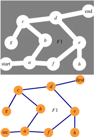
Figure 2.3 - Unit Disk Graph for the set of points given. Edges are included only for nodes whose half unit disks intersect. . . 19
Figure 2.4 - A Gabriel Graph Example:uandvare connected since no other vertex is within the disk. 20 Figure 2.5 - A Delaunay Triangulation Example: the triangletuvis included since no other vertex is within the disk. . . 20
Figure 2.6 - A graphic showing how a network topology can be visualized as a maze. . . 26
Figure 2.7 - Greedy routing example:xis the node nearest the destinationtof all the nodes directly connected tos, thereforesforwards the packet tox. . . 26
Figure 2.8 - A Greedy Routing example: y is the nearest to t ofx’s directly connected neighbors thereforexforwards the packet toy, and the packet continues to be greedily routed until reachingt. . . 27
Figure 2.9 - A Greedy Routing local minimum example: zis the closer than any directly connected node tot, therefore the packet cannot make greedy progress in the next hop, and greedy routing fails. . . 27
Figure 2.10 - A Greedy-Face-Greedy routing example. . . 30
Figure 2.11 - An example showing how a packet atpmay be forwarded to various different neighbors depending on the variant of greedy forwarding used. . . 32
Figure 2.12 - An image comparing the various face change point options. . . 34
Figure 2.13 - A basic Face Routing example. . . 34
Figure 2.14 - A FACE-2 routing example. . . 36
Figure 2.15 - A Bounded Face Routing example. . . 37
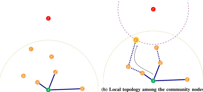
Figure 3.1 - An example showing how position exchange range, link range, the community, the neighborhood, and directly connected neighbors are defined. . . 47
Figure 3.2 - The unit disk graph among a set of aircraft positions. . . 49
Figure 3.4 - A diagram of the system-level architecture for each airborne platform (node). . . 51
Figure 3.5 - One-Way Connection Example. . . 58
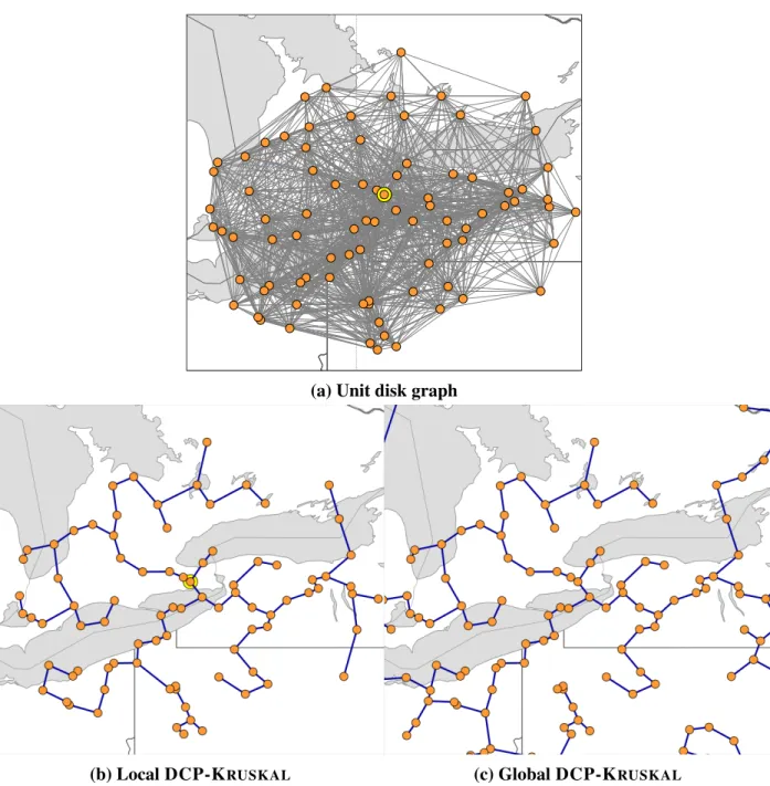
Figure 3.6 - The unit disk graph and the local and global graphs resulting from running the DCP-KRUSKALalgorithm. . . 62
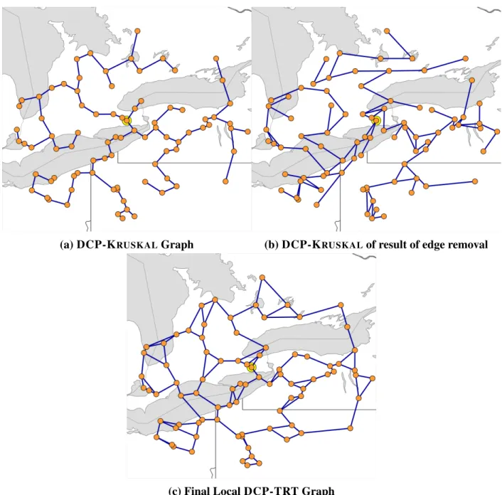
Figure 3.7 - The steps of computing DCP-TRT. . . 64
Figure 3.8 - The DCP-TRT topology among the sample set of nodes. . . 65
Figure 3.9 - The resulting global DCP-TRT topology. . . 66
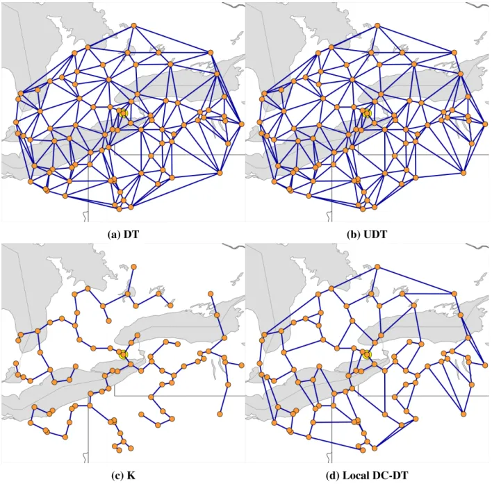
Figure 3.10 - The steps to computing the local DC-GG. . . 68
Figure 3.11 - The resulting global DC-GG topology. . . 69
Figure 3.12 - The unit disk graph and the local and global graphs resulting from running the DCP-KRUSKALalgorithm . . . 70
Figure 3.13 - The global DC-DT Topology. . . 71
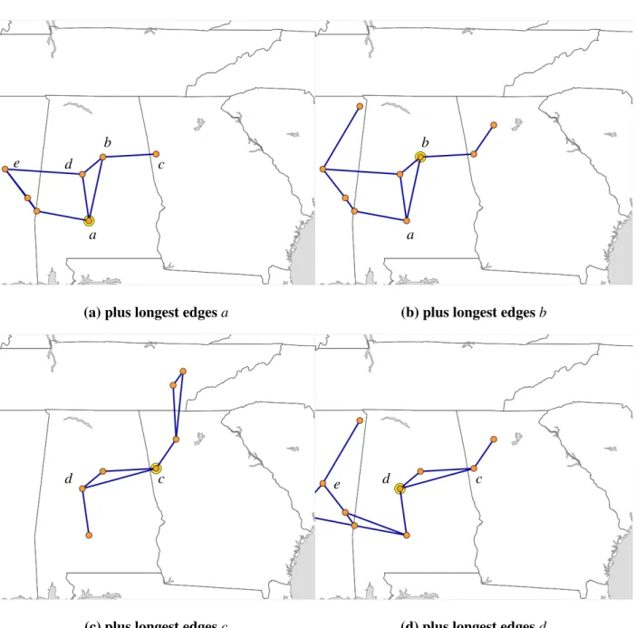
Figure 3.14 - The result nodes a, b, c, and d independently generating a local topology using the DCP-KRUSKAL algorithm given each node’s community members. The dashed circle shows the extent of the community from each node’s point of view. . . 72
Figure 3.15 - The result of these four nodes adding additional edges, longest first, to the topology graph. 73 Figure 3.16 - The resulting global non-planar topology. . . 74
Figure 3.17 - Computation of the local DCP-TRT topology at nodea. . . 75
Figure 3.18 - The computation of the local DCP-TRT topology at nodeb. . . 76
Figure 3.19 - The resulting global non-planar topology using DCP-TRT. . . 77
Figure 3.20 - A boundary ˜200 km offset from the continental United States border and coastline. . . . 78
Figure 3.21 - A visual comparison of the global continetal-scale topology resulting from each algorithm. 79 Figure 3.22 - An analysis of the number of connections. . . 82
Figure 3.23 - An analysis of the data links used and connected by each algorithm. . . 83
Figure 3.24 - An analysis of one-way connections. . . 84
Figure 3.25 - The mean length of a connection across algorithms. . . 85
Figure 3.26 - An analysis of the connected node pair metrics. . . 86
Figure 3.28 - The mean ratio of the number of edges added or removed in consecutive topologies, to
the number of edges in the topology. . . 88
Figure 3.29 - An analysis of link dynamicity. . . 88
Figure 3.30 - The ratio of the number of hops in the shortest path for each algorithm’s computed topology to the number of hops in the shortest path in the unit disk graph. . . 89
Figure 4.1 - An example of how face routing works with internal and external faces. . . 93
Figure 4.2 - An example of using an adaptive bounding circle to mitigate worst-case Face Routing situations, assuming there were many hops betweencandy. . . 94
Figure 4.3 - An example topology used for several examples in this chapter. . . 99
Figure 4.4 - An example of greedy routing in the example topology. . . 99
Figure 4.5 - A depiction of the bearing calculations. . . 101
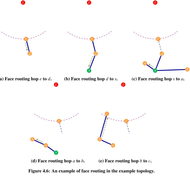
Figure 4.6 - An example of face routing in the example topology. . . 103
Figure 4.7 - An example of face routing when the destination is unreachable. . . 104
Figure 4.8 - An example of face routing motivating the need for the first edge to be included in the header. . . 105
Figure 4.9 - An example of a non-planar topology that thwarts face routing. The arrows trace the path of a packet starting atsand using the right-hand rule in an attempt to get tot. . 106
Figure 4.10 - An example of a non-planar topology where face routing fails to forward a packet to a reachable destination. . . 106
Figure 4.11 - An example of Greedy-Face-Greedy Routing. . . 107
Figure 4.12 - An example of a topology where the face exploration direction makes a difference. . . . 108
Figure 4.13 - An example of Adaptive Face Routing. . . 109
Figure 4.14 - A depiction of the notion of routing within an annulus centered at the destination. . . 110
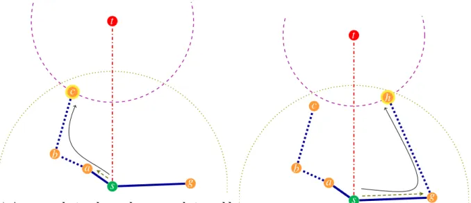
Figure 4.15 - An example motivating the advantages adding topology awareness to the normal Greedy mode. . . 118
Figure 4.16 - An example that motivates the need for the next topology-aware greedy hop to make progress toward the destination. . . 119
Figure 4.17 - Examples demonstrating selecting the face exploration direction based on the local topology. . . 122
Figure 4.19 - An example motivating the need for TAG to support fully dynamic topologies. . . 127
Figure 4.20 - An example of a topology that violates the Unit Disk Graph assumption. . . 130
Figure 4.21 - A comparison of hop stretch values as node density increases. . . 132
Figure 4.22 - A comparison of path stretch values as node density increases. . . 134
Figure 4.23 - A comparison of the hop stretch values with and without topology awareness. . . 135
Figure 4.24 - The network of aircraft used for the dynamic node simulation. A subset of 200 aircraft over the United States at 1:00 p.m. July 9, 2015. . . 137
Figure 4.25 - The network of aircraft used for the dynamic node simulation. A subset of 673 aircraft over the United States at 1:59:59 p.m. July 9, 2015. . . 137
Figure 4.26 - A plot of the CDF of the mean numbers of hops in an airborne network including hun-dreds of aircraft. (1 low-rate UDP flow per experiment, 1,000 experiments, 3 links per node, 1 hour simulated per experiment) . . . 138
Figure 5.1 - Diagram showing the relationship of the components that enable simulating wireless point to point links. . . 142
Figure 5.2 - The network of aircraft used for the global routing comparison. A subset of 609 aircraft spread across the United States at 9:00 a.m. July 9, 2015. Density: 9.47 nodes per unit disk. . . 145
Figure 5.3 - The CDF of the mean delay over all the packets in each flow. . . 147
Figure 5.4 - The CDF of the mean number of hops per packet in each flow. . . 148
Figure 5.5 - A snapshot of the network of aircraft used for the Large-Scale High-Density Experi-ment. A composite of the air traffic on July 16, 2015, at 12:00 noon and July 17, 2015, at 1:00 p.m. central time. . . 149
Figure 5.6 - The CDF of the mean one-way delay per packet for each flow in the Large-Scale High-Density simulations. . . 152
Figure 5.7 - The CDF of the mean number of hops per packet for each flow in the Large-Scale High-Density simulations. . . 153
Figure 5.8 - A scatter plot showing the correlation between the mean number of hops and the mean one-way delay. . . 154
Figure 5.9 - A snapshot of the initial network of aircraft used for the single high-rate flow experi-ments and the all pairs experiexperi-ments. The 264 nodes shown here span a large portion of the United States at 1:00 p.m. on Thursday, July 9, 2015. . . 155
Figure 5.11 - The throughput and number of hops for a one minute single high-rate UDP flow
exper-iment with a drop in throughput. . . 157
Figure 5.12 - A simulation showing how TAGs ability to begin sending packets over shorter paths can cause TCP to react negatively, decreasing the throughput potential for a high-rate flow.157 Figure 5.13 - The throughput and numbers of hops encountered after changing the duplicate ACK threshold to 10. . . 158
Figure 5.14 - A snapshot of the network of aircraft at the start of the long duration experiment. July 16, 2015 at 10:00:00 central time. . . 160
Figure 5.15 - A snapshot of the network of aircraft after 2 hours of the long duration experiment, July 16, 2015 at 12:00:00 central time. . . 160
Figure 5.16 - A plot of the throughput over the course of the long duration experiment. . . 161
Figure 5.17 - A snapshot of the network of aircraft used to analyze the effect of loss. . . 162
Figure 5.18 - The CDF of the throughput at various bit error rates (BER). . . 163
Figure 5.19 - The CDF of the packet delivery rate (PDR) at various bit error rates (BER). . . 165
Figure 5.20 - The CDF of the throughput for the All Node Pairs simulations. . . 167
LIST OF ABBREVIATIONS
ACK acknowledgment
AODV Ad-hoc On-demand Distance Vector
AFR Adaptive Face Routing
AO Adaptive Optics
ASDI Aircraft Situation Display to Industry
ATM Air Traffic Management
ATC Air Traffic Control
AAL American Airlines
ADS-B Automatic Dependent Surveillance - Broadcast
BER Bit Error Rate
BFR Bounded Face Routing
CPU Central Processing Unit
CT Central Time
DIR Compass Routing
CBTC Cone Based Topology Control
CBR Constant Bit Rate
CLDP Cross-link Detection Protocol CDF Cumulative Distribution Function CTR Critical Transmitting Range
dBmW decibels-milliWatts
DARPA Defense Advanced Research Projects Agency DC-DT Degree-Constrained Delaunay Triangulation DC-GG Degree-Constrained Gabriel Graph
DCP-KRUSKAL Degree-Constrained Planar Kruskal
DCP-TRT Degree-Constrained Planar Tree-based Reliable Topology
DT Delaunay Triangulation
DAL Delta Airlines
DSDV Destination Sequenced Distance Vector
DSR Dynamic Source Routing
ECEF Earth-centered Earth-fixed
EIGRP Enhanced Interior Gateway Routing Protocol
ERAST Environmental Research Aircraft and Sensor Technology
ENY Envoy
FR Face Routing
FAA Federal Aviation Administration FCC Federal Communications Commission FEC Forward Error Correction
FSO Free-Space Optics
FSOC Free-Space Optical Communication
FOENEX Free-space Optical Experimental Network Experiment
GG Gabriel Graph
GLSR Geographic Load Share Routing
Gb Gigabit
Gbps Gigabits per second
Gb/sec Gigabits per second
GB Gigabyte
GIG Global Information Grid
GPS Global Positioning System
GPSR Greedy Perimeter Stateless Routing
GR Greedy Routing
GFG Greedy-Face-Greedy
GOAFR Greedy Other Adaptive Face Routing GOAFR+ Greedy Other Adaptive Face Routing Plus GPVFR Greedy Path Vector Face Routing
ID Identifier
IP Internet Protocol Kbps kilobits per second
KB Kilobyte
km kilometer
LED light-emitting diod
LOS line of sight
LTE Long-Term Evolution
LLCD Lunar Laser Communications Demonstration LMST Local Minimum Spanning Tree
LTRT Local Tree-based Reliable Topology
MTU maximum transmission unit
MAC media access control
Mb Megabit
Mbps Megabits per second
MB Megabyte
ms Millisecond
MST Minimum Spanning Tree
MANET mobile ad-hoc network MFR Most Forward within Radius
MPR Multipoint Relay
MPLS Multiprotocol Label Switching
NASA National Aeronautics and Space Administration
NAS National Airspace System
NCO Network Centric Operation
OPVFR Oblivious Path Vector Face Routing OSPF Open Shortest Path First
OAFR Other Adaptive Face Routing OBFR Other Bounded Face Routing
OFR Other Face Routing
PT Pacific Time
PDR Packet Delivery Ratio
PER Packet Error Rate
PVEX Path Vector Exchange Protocol PAT Position Acquisition and Tracking
PIF power in the fiber
RF radio frequency
RNG Relative Neighborhood Graph
RERR Route Error
RREP Route Reply
RREQ Route Request
s Second
SINR Signal to Interference and Noise Ratio
SWA Southwest Airlines
TAG Topology Aware Geographic Routing TCP Transmission Control Protocol TRT Tree-based Reliable Topology
TTL Time to live
UDT Unit Delaunay Triangulation
UDG Unit Disk Graph
UK United Kingdom
UPS United Parcel Service
UTC Coordinated Universal Time
UAV Unmanned Aerial Vehicle
CHAPTER 1: INTRODUCTION
As wireless digital communication networks mature and advance, their reach has been extending into previously unimaginable regions, including outer space [BSM+09], under water [DSSM15], and under-ground (where the propagation medium is the soil) [CaRCR15]. Yet even more fascinating has been the re-cent surge of interest in forming networks in the Earth’s stratosphere, that has propelled the field of Airborne Networking from its origins inside military research labs out onto the center stage. Well-known companies like Google and Facebook are making huge investments in their own large-scale airborne networks as they race to define and control these futuristic networks in the skies.
An airborne network is a digital communication network which includes nodes, such as balloons, blimps, or fixed-wing aircraft, that are airborne. Among the many challenges associated with these highly-dynamic networks is that of forming long-range high-bandwidth connections between them, and efficiently routing data over those connections in a manner that is scalable to potentially tens of thousands of nodes. Directional data links are data links which focus their transmissions in a certain direction. These links can facilitate the required high-rate connections over long ranges, but their use violates many of the assumptions made by traditional networking protocols. Further, these directional data links require explicit management of the network topology, so that it can quickly adapt and evolve as nodes join, swiftly move within, and leave the network. These frequent changes to the network topology induce large amounts of routing overhead and packet loss even in routing protocols designed for mobile networks. This dissertation details a distributed topology management framework and a geographic routing algorithm capable of efficiently routing high-bandwidth traffic in a large-scale airborne network connected by directional data links. The effectiveness of these algorithms is demonstrated through a series of experiments that simulate the formation of an airborne network of commercial aircraft tracing the paths of actual flights in the United States airspace.
1.1 Airborne Networks of Balloons, Drones, and Commercial Aircraft
it is estimated that 31% of the population do not even live within range of a 3G mobile network [Fac16]. Building the traditional infrastructure required to connect these users to the Internet is an extremely expen-sive and slow process; land rights must be purchased, cables must be laid or towers erected, and costly communications equipment must be installed. These barriers may be one of the reasons that Facebook and Google are looking to the stratosphere for a creative solution to the problem of connecting more users (and customers) to the Internet.
In June 2013 Google announced their plans to create an airborne network of high-flying balloons to provide internet service to users on the ground throughout the world [TP13], [DTBW13]. Facebook quickly followed suit, purchasing UK-based Ascenta [Gar14], a maker of solar-powered drones, and announcing that they were working on ways to beam Internet to people from the sky [Kel14]. Since that time both com-panies have made significant progress toward their goals, with Google launching balloons in New Zealand, California, and Brazil [Sim16], and Facebook testing its full-scale solar-powered Internet drone that may one day stay aloft for three to six months[New16].
Although both approaches are unique (each with its own challenges), the fundamental idea is the same: form a high-capacity backbone network between airborne nodes, connect it to ground station gateways, and provide Internet connections from each node to users on the ground (using an additional communication system). A common challenge to either proposal, however, is the sheer scale of such a network. According to Google, each of the balloons in their proposed architecture can provide coverage to a ground area with a diameter of about 40 km [Mur15]. This means that to actually provide Internet connections to just the continental United States, Google would need over 6,000 precisely-positioned balloons.
1.2 Free-Space Optical Communication Links
Free-space optical communication (FSO) is expected to be an essential technology in achieving the high-bandwidth connections over long distances required for the airborne network backbone. Google is investi-gating the use of ultra-bright light-emitting diodes (LEDs) for communication between balloons [DTBW13], and Facebook claims to have developed free-space laser transceivers that improve upon the state-of-the-art by an order of magnitude, yielding data rates in the tens of Gbps [Mag]. The United States Armed Forces are also linking aircraft together with low-power infrared lasers. A recently completed Defense Advanced Research Projects Agency (DARPA) program demonstrated air-to-air connections with ranges up to 200 km and air-to-ground connections with slant ranges (line-of-sight distance between data links at different altitudes) up to 130 km while maintaining data rates from 3 to 9 Gb/sec using a hybrid FSO/RF link [DOD13], [SPM+11], [APC+12].
Conveniently, free-space optical communication links do not require a Federal Communications Com-mission (FCC) license or spectrum allocation, and are smaller, lighter, more secure, and more power efficient than high-bandwidth radio frequency (RF) links. FSO links, however, are very sensitive to atmospheric tur-bulence, and line-of-sight obstructions (such as clouds). It has been shown that a combination of Adaptive Optics (AO), Optical Automatic Gain Control (OAGC), and Forward Error Correction (FEC) can overcome the effects of the severe atmospheric turbulence which impacts these links [SPM+11]. Other techniques such as link layer retransmissions can further improve the link quality. Note, also, that atmospheric turbu-lence and cloud obstructions are less prominent at high altitudes where it is anticipated that the bulk of the airborne network connections will be formed. In addition, the topology management framework (discussed next) could take cloud positions into account, and route around them as in [JRO+09].
1.3 Distributed Explicit Topology Management
In traditional wireless networks, where omnidirectional communications are the norm, topology control involves coordinating the transmission power of network nodes to generate a topology with certain prop-erties [San05]. Topology control employed on a sensor network, for example, may be used to manage a network such that connectivity to all nodes is maintained, but power consumption is minimized. The use of directional FSO links drives the need for a topology management framework which is related to topol-ogy control, but which explicitly determines which nodes should point to and connect with one another. In addition, when using directional links, the degree, or number of incident edges at a node in the topology, is limited to the number of physical directional data links at that node. Thus, the topology management framework must also guarantee that degree constraints are met while seeking to form a desirable global topology.
Imagine a centralized topology management framework where, once connected, all nodes would send their position and connection information through the network to a selected control node. This special control node could determine the best global topology for the network and then command each node to make appropriate connectivity changes to realize that topology. This design, however, has several disadvantages besides the fact that it presupposes the connectivity of the nodes. First, it creates a single point of failure at the control node for the network. Next, significant amounts of extra overhead would be required to send the position information of all nodes to the control node, potentially causing congestion on links near the control node. Further, this design places much of the computational burden on the single control node, requiring it to compute a global topology that includes all the nodes. Lastly, and implicit in each of the previous disadvantages, is the issue of scalability. As the number of nodes in a network managed by such a scheme increase, the bandwidth would eventually be completely consumed in just managing the topology of the network. Clearly, a distributed solution is warranted, especially when networks of tens of thousands of nodes are desired.
overhead of such a scheme, in fact, would be the cost of exchanging position information with nearby nodes (something already done by commercial aircraft using a separate system). In addition, the only associated “costs” could be a slight decrease in the number of connections formed, leaving some links unused, and an increase in the frequency of connection changes. Could the topology actually be managed in this way? One of the main contributions of this work is a topology management framework which operates exactly as described above. The design of this distributed management framework and the topology generation algorithms it requires are detailed in Chapter 3.
1.4 Routing in Large-Scale Airborne Networks
A network formed by connecting aircraft using a limited number of directional data links is necessarily highly-dynamic. Frequent changes to the topology are required as nodes join, move within, and leave the network. Nodes that are not directly connected in this dynamic topology must communicate by relaying their messages through a series of intermediate nodes, each acting as a router. A routing protocol or algorithm is needed to determine, at each node along that path, where the message should be forwarded next.
Mobile Ad-hoc network (MANET) routing protocols are designed to support networks formed among mobile nodes, but even these protocols often fail to efficiently route packets in highly-dynamic, large-scale networks [NAJ15]. Consider, for example, a network of ten thousand mobile nodes, and two nodes on opposite edges of this network attempting to communicate. A reactive MANET routing protocol (one that seeks to establish routes “on demand”), will need to buffer packets until it can find a path through the network to the distant node. Once a path is found packets may begin flowing. However, unless the nodes along the path are essentially stationary, there is a high probability the path will quickly become invalid. All it takes to make the path obsolete is one node along the path to leave the network or move out of range of an adjacent node supporting the path. Packets must then be delayed or dropped while the path is repaired, requiring extra management packets be sent, and increasing overhead.
actually arrive at their intended destinations because the routing information so quickly becomes stale. In contrast, geographic routing protocols don’t actively maintain routes, and never need to determine or repair paths through the network.
Geographic routing protocols (or position-based routing protocols) forward packets based on the geo-graphic position of the destination, not by identity or address. The nodes supporting a geogeo-graphic routing protocol need only store minimal information about other nearby nodes, and never global topology or path information. There is no need to set up a path because hop-by-hop decisions are made about where the packet should be forwarded next. This allows the protocols to quickly adapt to changes in the network while avoiding stale information.
There are two main approaches to geographic routing: greedy routing and face routing. In greedy routing the packet is forwarded at each hop to whichever directly connected neighbor is nearest the packet’s destination [Fin87]. Unfortunately, if the packet reaches a node whose neighbors are all further away from the destination than it is, the packet has reached a dead end (local minimum), and cannot make greedy progress.
Face Routing (Compass Routing II) is the other main geographic routing approach [KSU99]. Face routing makes use of the right-hand rule that states that the entire boundary of any face of a planar graph can traced by, at each vertex proceeding along the incident edge that is sequentially counterclockwise about the vertex from the arrival edge (aka at each vertex/roundabout always take the immediate right turn). Various face routing methods utilize the right-hand rule to traverse individual faces and then switch to the next face along a path of faces from the source to the destination.
Greedy and face routing are often combined producing so-called greedy-face-greedy protocols. These protocols start routing greedily until a local minimum is reached, at which point face routing is used to route around the face between the local minimum and the destination. Greedy routing then resumes.
even while a packet is in flight, and can work with topologies formed by directional links. Such a routing algorithm could also benefit from the local topology information available at the nodes as a by-product of topology management.
1.5 Thesis Statement
A topology management framework and a routing algorithm can be developed that are capable of con-necting thousands of commercial aircraft, flying normal routes, into a large-scale airborne network sufficient to support tens of thousands of 1 Mbps data flows.
1.6 Summary of Main Contributions
In support of this thesis, two algorithms are designed that are sufficient to connect thousands of airborne nodes into a topology which is actively managed over time and route large amounts of data between those airborne nodes. In addition, these algorithms are implemented and tested via simulation. The results of these simulations, where nodes follow actual aircraft trajectories, demonstrate the effectiveness of these algorithms and the capability of the airborne network. A summary of each of these contributions is given below.
1.6.1 Distributed Topology Management Framework
1.6.2 Topology Aware Geographic Routing Algorithm
Routing within large mobile networks is challenging, especially at high data rates and when node move-ment is highly dynamic. The next contribution of this work is Topology Aware Geographic Routing (TAG), a position-based routing algorithm that strategically uses local topology information to make better local forwarding decisions, decreasing the number of hops required to deliver a packet when compared with other geographic routing protocols, while essentially guaranteeing delivery, and sending no overhead packets. In addition TAG is able to reliably deliver packets even in topologies that violate the often used but unreal-istic unit disk graph and quasi-static assumptions. A variety of simulations support the claim that TAG outperforms GOAFR+, GFG, and OLSR in both theoretical environments and in a simulated, real-world, continental-scale airborne network.
1.7 Organization of Dissertation
The remainder of this dissertation is organized as follows.
Chapter 2 gives an in-depth look at several pertinent topic areas and provides an overview of related research that has been conducted.
Next, in Chapter 3, the new distributed topology management framework is detailed, and experiment results that compare various topology generation algorithms are presented.
Chapter 4 then details the design of a new topology aware geographic routing protocol that is able to route packets in the highly-dynamic airborne network topology while using local topology information (obtained as by-product of topology management) to improve its efficiency. Results of simulations compar-ing this new protocol to other state-of-the-art geographic routcompar-ing protocols in an airborne network are also presented.
The results of a variety of simulations demonstrating the effectiveness of the resulting airborne network system are then presented in Chapter 5. These simulations utilize actual flight path data collected by the FAA to replay realistic node movements.
CHAPTER 2: BACKGROUND AND RELATED WORK
This chapter begins by introducing the reader to the burgeoning field of airborne networking, then briefly introduces various topics pertinent to understanding this dissertation. A discussion of works related to this research follows, where specific implementations of many of the topics covered in the background section are described.
2.1 Background
2.1.1 Airborne Networks
An airborne network has been loosely defined as an infrastructure that provides communication trans-port services through at least one node that is a platform capable of flight [USA07]. Until recently, most airborne networking research was conducted by military research facilities and defense contractors. Many of these military “airborne networks” included only a single airborne node, and simulated networks often included only a couple dozen nodes. The last few years, however, have seen a huge increase in both the scale of proposed airborne networks and the level of interest in airborne networking. This surge can be largely attributed to Google and Facebook who have allocated large amounts of time and money in an attempt to build the first large-scale civilian airborne network. The airborne networks being designed by these com-panies include not dozens, but thousands or even tens of thousands of nodes spread around the globe. The following sections provide more detail about these two main types of airborne networks, namely Military Airborne Networks and Civilian Airborne Networks.
2.1.1.1 Military Airborne Networks
To achieve this vision, the Global Information Grid (GIG) [DOD05b] was proposed. The GIG is an all-encompassing communications plan, that includes everything needed to collect, process, manage, and disseminate information to warfighters, decision makers, and support personnel. The GIG includes a space backbone layer, with communication satellites, a terrestrial network layer, providing surface connectivity, and an airborne networking layer, connected to both space and surface networks. Airborne networks are thus an integral part of the grid and a fundamental component of the network-centric vision.
Military airborne networks can be further divided into two broad classes: airborne subnets, and backbone networks. Airborne subnets include several existing tactical and sensor networks. These various networks connect a small set of airborne platforms together to support a specific task. In contrast, backbone airborne networks form a high-bandwidth backbone Internet Protocol (IP) network to interconnect satellite networks, airborne subnets, sea and ground based mobile ad-hoc networks, and fixed terrestrial networks into a single network. Besides enabling communication between forces, these backbone networks are also a key to operating under satellite denied conditions, a current concern of the Pentagon.
2.1.1.2 Civilian Airborne Networks
As mentioned previously, both Google and Facebook are progressing their own the massive civilian airborne networks that they hope will expand the reach of the Internet without the need of costly terrestrial infrastructure. These companies, however, were not the first inspired by the vision of providing high-speed internet from semi-permanent relay nodes in the stratosphere. Several companies have previously attempted to bring similar ideas to market.
rapid expansion of terrestrial wired and wireless networks leading to a failure of their business models, and the impact of the terrorist attacks on September 11, 2001, on the aviation industry and the economy.
Over the next decade, similar projects continued to make small advances in delivering telecommunica-tions from high-altitude airborne platforms, including projects in Japan, Korea, and Europe, and the United States. AeroVironment Inc., for example, worked with the National Aeronautics and Space Administra-tion (NASA) in the Environmental Research Aircraft and Sensor Technology (ERAST) program to develop Helios, a high-altitude unmanned aerial vehicle (UAV) that was intended to perform atmospheric research tasks and serve as a communications platform. Unfortunately, the Helios Prototype broke up and fell into the ocean in 2003, and the entire NASA ERAST program was terminated [NBPD+04].
A decade later (2013) Google Inc. announced its intent to form an airborne network of high-altitude balloons that would provide Internet service to users on the ground, including those living in remote ar-eas [Sim16]. These balloons would float freely in the stratosphere, circling the globe, while forming a network among themselves. The balloons would provide communication services to every corner of the globe, including places with no current communications infrastructure. Project Loon, as it is called, has performed tests in New Zealand, Brazil, and Australia. Patent documents reveal that Google plans to create a hierarchy of balloons, with super-node balloons forming a backbone using free-space optical links, and sub-nodes connecting to the backbone and the ground antennas using radio frequency (RF) [DTBW13]. Another patent also reveals that Google anticipates clumping balloons over certain areas to meet expected historical demand, or to facilitate advance requests for service during special events [TP13]. Project Loon is currently battling for permits to run test flights over the United States. It is quite possible that Google will actually bring this seemingly “Loon-y” idea to fruition.
using proprietary laser transceivers [Mag].
2.1.2 The National Airspace System (NAS)
This dissertation focuses on large-scale high-capacity airborne networks. One such network could be formed among commercial aircraft that are already flying in the skies every day. To simulate a realistic large-scale airborne network, that is large-scale both in numbers of nodes and geography, our simulations play back the actual flight paths of air traffic within the United States. This section gives an overview of the air traffic within the United States and how these data were obtained.
Figure 2.1: A view of the number flights in the NAS over 24 hours, stratified by the company designa-tion in the call sign. Time on the x-axis is UTC-6 (Central Time).
car-riers can be seen in the bands starting at the bottom with American Airlines (AAL), followed by Southwest Airlines (SWA), then Delta Airlines (DAL), etc. Other airline abbreviations may not appear as familiar such as ENY, the symbol for Envoy Airlines. Envoy is a regional air carrier that operates under the American Eagle brand. The “other” band at the top combines all the remaining airlines together whose fraction of flights is too small to plot individually. This includes international airlines, small charter airlines, etc. One other interesting feature to note is the contribution of the cargo airlines. This can be seen on the left-hand side of the figure around 4 a.m. Notice the two bands that widen as the most others shrink. These are the hundreds of FedEx and United Parcel Service (UPS) flights that dominate the early morning air traffic, ensuring that packages are ready to be sent out on trucks at the crack of dawn. If a large percentage of the commercial aircraft flying in the early morning hours (including cargo aircraft) participate in the airborne network, most of the nodes will be able to remain connected to the network. However, it is unlikely that the sparse commercial air-traffic in these early-morning hours will be sufficient to provide reliable network connections to areas far removed from the busiest air-traffic routes. For this reason, it may be beneficial to also employ a set of drone aircraft to fill gaps in the network coverage during these times.
Figure 2.2 shows a similar view of the air traffic, but over the course of a week (July 1 to July 7, 2015). The diurnal variation (daily cycle) is quite evident, with much fewer flights during the early morning hours. Minor variations can be seen from day to day, but the general patterns are consistent. Notice also, the smaller number of flights on the July 4th weekend.
2.1.2.1 ADS-B
An important part of the topology management scheme introduced in Chapter 3 is the exchange of po-sition information with nearby nodes. Automatic Dependent Surveillance - Broadcast (ADS-B) essentially already performs this function for commercial aircraft, a fact we capitalize on.
ADS-B is a new Air Traffic Management and Control (ATM/ATC) surveillance system that has been certified as a viable replacement for the FAA’s traditional radar-based systems. In the new system, each air-craft broadcasts a radio transmission containing its current position, ground speed, identification, and other air traffic management information approximately once a second [FAA05]. These messages are received by ATC ground stations and other ADS-B equipped aircraft within a 100 to 200 nautical mile range (185 to 370 km or 115 to 230 statute miles) [SLM15][FAA05].
The new system provides data faster and at a higher resolution than traditional radar systems, enabling closer spacing of aircraft and decreased congestion. It also has the added benefit of improving the situa-tional awareness of pilots, who can now learn the positions of nearby aircraft and view the air traffic on an integrated display. Further, ADS-B decreases the reliance on a ground infrastructure, and ADS-B ground station receivers are easier and less expensive to deploy than radar stations. Because of these benefits, the FAA has mandated that most aircraft operating in the controlled United States airspace must be equipped to send ADS-B messages by January 1, 2020. [FAA10]
2.1.2.2 Aircraft Situation Display to Industry (ASDI)
In order to replay aircraft trajectories for airborne network simulations, Federal Aviation Administration (FAA) Aircraft Situation Display to Industry (ASDI) data is used.
2.1.3 Directional Communication Links
As mobile users consume higher and higher amounts of network bandwidth, cost effective alternatives to legacy wireless links are needed. Traditional ground-based wireless RF networks are bound by provable limits of per-node throughput [GK00], and will likely not scale to meet future demands. The directional communication links described in this section are key to enabling high-capacity airborne networks.
An antenna that radiates uniformly in all directions in a plane is called an omnidirectional antenna. Omnidirectional antennas are commonly used in radios, cell phones, wireless networks, etc. In contrast, an antenna that radiates or receives power more efficiently in some directions than in others is called a directional antenna. Directional antennas can both improve the transmission and reception of communica-tions and reduce interference from extraneous sources. The improved transmission and reception allow for signals to be sent over longer distances, with fewer errors, or at higher rates. In addition, directional links provide increased security, significantly limiting the potential for communication detection and interception. This is a double-edged sword, however, as protocols that rely on overhearing their neighbor’s transmissions (snooping) won’t function well in a network of directional links.
The measurement used to describe the efficiency of an antenna is called the antenna’s power gain or sim-plygain.Transmit antenna gainmeasures how well an antenna converts input power into radio waves, while receive antenna gainmeasures how well the antenna converts radio waves into electrical power. Most direc-tional antennas exhibit maximum transmit and receive gain in a single direction. These antennas are called unidirectional antennas. Antennas that can change the direction of their focused transmission are called steerable directional antennas. These types of antennas can be eithermechanically steeredorelectronically steered. Mechanically steered antennas are mounted on a gimbal or similar construction, that can turn the antenna, effectively rotating the antennas radiation pattern relative to the platform. Electronically steered antennas (also called steerable beam directional antennas, phased array antennas, smart beam-steering an-tennas, or smart antennas) can be steered to point in different directions by independently controlling the phases of each antenna in an array of antennas, such that constructive interference causes more power to radiate in certain directions and destructive interference attenuates the signal in other directions.
2.1.3.1 Directional Radio Frequency (RF) Communication Links
Directional RF links are generally characterized as being extremely reliable, even in the presence of clouds, fog, or atmospheric turbulence. They can operate over long ranges (e.g. 200 km), and at fairly high rates (e.g. 274 Mbps). Armed forces from various countries use (mechanically and electronically) steerable directional radio frequency (RF) links [BRMD07] to create high-bandwidth connections among aircraft, and between aircraft and ground stations. The Mini-T2 system [L3:11], for example, can achieve data rates up to 274 Mbps at ranges up to 150 nautical miles (278 km, 173 statute miles). Also, DARPA is currently developing an RF link that can enable communication between an aircraft and ground station over long ranges at 100 Gb/s [Kel15]. Unfortunately, however, high-frequency RF links can suffer substantial attenuation from rain, depending on the rain drop size distribution and the rain field characteristics. Also, since radio frequency bands are regulated by governments, the operation of RF links requires a spectrum allocation. In the United States, the Federal Communications Commission (FCC) manages and regulates spectrum use. Because of the scarcity of available spectrum, it can be extremely difficult and costly to secure the large allocation needed for a new high-rate RF system.
2.1.3.2 Free-Space Optical Communication Links
Free-Space Optical Communication (FSO) links use pulses of light emitted from an infrared laser to form a wireless optical communication channel (like fiber-optics without the fiber). The main advantage of these types of links is their high capacity. Data rates up to 1.28 Tbps (Terabits per second) have been demon-strated over a short distance of 200 meters [CAC+09]. However, other advantages abound, including full duplex operation, low interference, no Federal Communications Commission (FCC) license requirement, no spectrum scarcity. Further, the extremely narrow beamwidth of the laser makes interception of transmissions by a third party very difficult, yielding a highly secure link. FSO links are also generally lighter, smaller, and require less power than RF links. Interestingly, since the propagation speed through fiber is slightly slower than in air, FSO links can actually send data faster than fiber-optics links.
unobstructed line-of-sight (LOS) between FSO links, and thus their optical signals are severely attenuated by fog, haze, and clouds. Finally, the narrowness of the laser beam requires extremely accurate pointing. FSO links attached to or tracking mobile platforms (such as aircraft) must be mounted on a precision gimbal, and employ a sophisticated Pointing Acquisition and Tracking System (PAT) [RED13] to acquire connections and to continuously adjust their pointing to maintain a lock on their target.
Despite these limitations, Free-Space Optical Communication links are seen by many to be an “essential enabler” of airborne networks [BRSS12]. Many of the limitations of these links disappear or are reduced at high altitudes, making FSO links a natural choice for connecting a high-capacity airborne network or even a space network. In fact, NASA is already using laser communications in space. The recently completed the Lunar Laser Communications Demonstration (LLCD) [BSM+09] proved that it is possible to receive, through a transportable ground terminal, high-rate laser communications from a satellite in lunar orbit over a quarter million miles away.
2.1.3.3 Hybrid Free-Space Optical Radio Frequency (Hybrid FSO/RF) Communication Links
There is a natural synergy between directional RF and FSO links that can be exploited by using them in tandem [DTS05]. RF links generally have a smaller capacity than FSO links but are generally more dependable. FSO links have a huge capacity, but are not as dependable, especially in the face of excessive atmospheric turbulence. By combining an FSO and an RF link into a Hybrid link the benefits of both technologies can be enjoyed. The FSO link can transmit large amounts of data when available, and the dependable RF channel can be used for critical control messages, acknowledgments, or for exchanging data or dropped packets if the FSO link is momentarily down. Adding to the synergy, the link types complement one another where weather effects are concerned. High-capacity directional RF links perform poorly in rain, but in the same conditions, FSO links experience only a moderate attenuation. Similarly, FSO link performance is severely impacted by fog or haze, but RF link performance is not. Interestingly, the reason fog impacts an FSO connection is that the radii of the water droplets in fog are about the same size as the infrared wavelength, causing the infrared light to scatter [GW02]. Similarly, RF links perform poorly in rain, because the sizes of the raindrops are close to the wavelengths of microwave signals.
from 90 km to 130 km, and an air-to-air connection maintaining a data rate of 6 Gbps at ranges from 50 to 212 km [YHSJ15][DOD13]. These ranges and rates are possible because of the use of cutting-edge adaptive optics (AO) and optical automatic gain control (OAGC) demonstrated by DARPAs Optical RF Communications Adjunct (ORCA) and Free-space Optical Experimental Network Experiment (FOENEX) projects [SPM+11]. Adaptive optics corrects optical distortions caused by atmospheric turbulence, while OAGC helps to keep the incoming signal levels consistent. Performance is further improved using a link layer retransmission scheme, that detects the onset of scintillation events and quickly retransmits dropped packets over the RF link.
Many of the experiments conducted as a part of this research use simulated links that emulate the fun-damental characteristics of these hybrid FSO/RF links, but generally in pristine environments.
2.1.4 Network Topology
A network topology indicates the arrangement of communication links between nodes in a network. For traditional wired networks, the network topology is determined by the physical cables connecting network nodes, and it is generally fairly static. In contrast, most wireless networks use omnidirectional antennas to transmit their messages in all directions to all nodes within some maximum range. If nodes are mobile, the topology is dynamic and is implicitly determined by the environment, the transmission ranges (affected by the transmission power), and the node movement. Indirectional networks(networks that utilize steerable directional communication links, such as FSO links) a topology must be explicitly determined and managed as nodes move. Nodes have a finite number of links, and therefore a finite number directly connected neighbors. Each directional antenna or free-space optical terminal for these links must be commanded to point at its intended neighbor, who also must point one of its links back. More importantly, each node must determine which of its potentially many neighbors it should directly connect with.
This following sections explore some concepts relating to the network topology graph and controlling the topology.
2.1.4.1 Unit Disk Graph
using disks with a radius of one unit, in which case the graph would include edges between a node and any node within its disk. Alternatively, the graph can be visualized using disks with a radius of half a unit (0.5), in which case the graph would include edges between any nodes whose disks intersect. Figure 2.3 shows a simple unit disk graph for a set of nodes that uses the latter visualization convention (half unit disks). Notice that the graph includes an edge between any two nodes whose half unit disks intersect (e.g. nodesxandy), and does not include an edge between nodes whose disks do not intersect (e.g. nodesyandz). Formally a unit disk graph can be defined as follows. GivenP, a set of points in a plane, the unit disk graphU(P) includes a vertex for each point and an edge(u,v) between a pair of vertices if and only ifdist(u,v)≤1, wheredist(u,v)is the Euclidean separation distance betweenuandv. Notice, that the unit disk graph places no constraint on the degree of each node. In a unit disk graph, a node is always connected to all other nodes within the maximum transmission range (that has been normalized to 1 unit), and is never connected to any node outside that range [KWZ03a]. The unit disk graph is an accurate model of a 2-dimensional broadcast wireless network if: (1) all nodes have the same transmission power and the same receive gain, yielding the same maximum transmission radius, (2) every node’s transmission pattern is a perfect circle (each node transmits and receives equally in every direction), and (3) there are no radio-opaque obstacles and no multipathing to interfere with this perfect transmission. While convenient for theoretical analysis, unit disk graphs rarely match real-world wireless network topologies [KWZ03a], [KGKS05b], [KGKS05a]. In this research, the Unit Disk Graph will be utilized to represent all of the connections that could potentially be formed among a set of nodes. Since not all of these connections can actually be formed simultaneously, an appropriate degree-constrained subgraph of the unit disk graph must be determined.
x y
z
2.1.4.2 Planar Graph
Some techniques (e.g. face routing) used in this research require graphs that are guaranteed to be planar. Aplanar graphis a graph that can be drawn in a plane without any of its edges crossing. If the positions of vertices of a non-planar graph are fixed in a 2-dimensional plane, a planar subgraph can be generated from the original graph by removing an edge for each pair of edges that intersect. There are many algorithms for generating a planar subgraph. One such algorithm is the Gabriel Graph (GG). Remember that a disk is the region of a plane bounded by a circle. Aclosed diskincludes points on the circle (includes all points≤the radius). Letdisk(u,v)be a closed disk that has the line segment uvas a diameter. Given a set of pointsP, the Gabriel Graph includes an edge(u,v)if and only ifdisk(u,v)contains no other points inP. Figure 2.4 displays the edge(u,v), for example, since nodew(and all other nodes inP) are located outside of the disk of which the line segment betweenuandvis a diameter. Ifwwere located inside the disk, the edge(u,v) would not be included in the Gabriel Graph.
u v
w
Figure 2.4: A Gabriel Graph Example:uandvare connected since no other vertex is within the disk.
Delaunay Triangulation is another algorithm that can be used to generate a planar subgraph of an input graph. Delaunay Triangulation creates a triangulation for an input set of points. A circumcircle is a circle that passes through all the vertices of a given polygon. Given a set of pointsP, the Delaunay Triangulation includes a triangletuvif and only if the circumcircle of that triangle contains no other points inP. Figure 2.5 shows that the resulting triangulation would include triangletuv, sincew(and all other nodes inP) are located outside of the circumcircle. The Gabriel Graph is a subgraph of Delaunay Triangulation.
t
u v
w
Figure 2.5: A Delaunay Triangulation Example: the triangletuvis included since no other vertex is within the disk.
faces, that make up a graph, but always also one extra unbounded exterior face that encompasses all other space.
2.1.4.3 Topology Control
Topology Control in wireless ad hoc network and sensor networks has been studied extensively. How-ever, the main focus has been on networks using standard omnidirectional antennas. In these networks, topology control involves adjusting the transmission power of nodes to achieve a global topology that is connected and optimized for some metric, such as minimal energy use. In [San05] Santi gives a thorough overview of Topology Control research, dividing the field into Homogeneous and Nonhomogeneous meth-ods, where the homogeneity refers to the transmit power or range of the nodes. In homogeneous topology control, the Critical Transmitting Range (CTR) is the common minimum range at which all nodes will transmit, such that the network remains connected. Nonhomogeneous methods allow for each node to be assigned a unique transmit range and associated transmission power, enabling even more specific control of the topology. Santi further divides nonhomogeneous methods into Location-Based, Direction-based, and Neighbor-based distributed protocols. In Chapter 3 a distributed topology control method is introduced that explicitly controls the topology of a network of mobile nodes connected using directional links.
2.1.5 Routing in Mobile Ad hoc Networks
Delivering messages between nodes in an ad hoc network is an important and difficult problem. In the routing problem, a source nodesand a destination or target nodetare elements of a set of pointsP, and the nodesis to send a message to the nodet.
2.1.5.1 Topology-Based Routing
Topology-based routing protocols use link information that exists in the network to make forwarding decisions. Topology-based protocols for mobile ad hoc networks can be further divided into three groups: (1) Proactive protocols, (2) Reactive (On Demand) protocols, and (3) Hybrid protocols.
Proactive MANET routing protocols use traditional routing algorithms to maintain paths (routes) be-tween every pair of nodes in a network. Routes are proactively maintained bebe-tween every pair of nodes, ensuring that packets flowing over a previously unused path can begin flowing without delay. Unfortunately, proactive protocols require that numerous control messages be sent to update the routing tables. These con-trol messages, or overhead messages, may occupy an unacceptably large fraction of the network bandwidth, actively maintaining paths between nodes that never directly communicate. This overhead for proactive pro-tocols, however, generally remains fairly constant as node mobility increases. Optimized Link State Routing Protocol (OLSR) [JMC+01] and Destination-Sequenced Distance Vector (DSDV) [PB94] are examples of proactive MANET routing protocols. OLSR is a version of the classical link state algorithm that has been optimized for mobile networks. In OLSR each node selects Multipoint relays (MPRs) and uses only these nodes to broadcast control traffic to the network, significantly reducing the number of transmissions when compared with traditional flooding. In addition, link state information is only generated by MPRs, mini-mizing the number of OLSR control messages. DSDV, on the other hand, is based on the distance vector algorithm but it adds sequence numbers to each table entry to avoid routing loops as the network topology changes.