IMPROVED ENCODING FOR COMPRESSED TEXTURES
Pavel Krajˇcevski
A dissertation submitted to the faculty of the University of North Carolina at Chapel Hill in partial fulfillment of the requirements for the degree of Doctor of Philosophy in the
Department of Computer Science in the College of Arts and Sciences.
Chapel Hill 2016
Approved by: Dinesh Manocha
Ming C. Lin
Ketan Mayer-Patel
Matt Pharr
ABSTRACT
PAVEL KRAJCEVSKI: Improved Encoding for Compressed Textures (Under the direction of Dinesh Manocha)
For the past few decades, graphics hardware has supported mapping a two dimensional image, or texture, onto a three dimensional surface to add detail during rendering. The complexity of modern applications using interactive graphics hardware have created an explosion of the amount of data needed to represent these images. In order to alleviate the amount of memory required to store and transmit textures, graphics hardware manufacturers have introduced hardware decompression units into the texturing pipeline. Textures may now be stored as compressed in memory and decoded at run-time in order to access the pixel data. In order to encode images to be used with these hardware features, many compression algorithms are run offline as a preprocessing step, often times the most time-consuming step in the asset preparation pipeline.
This research presents several techniques to quickly serve compressed texture data. With the goal of interactive compression rates while maintaining compression quality, three algorithms are presented in the class of endpoint compression formats. The first uses intensity dilation to estimate compression parameters for low-frequency signal-modulated compressed textures and offers up to a 3X improvement in compression speed. The second, FasTC, shows that by estimating the final compression parameters, partition-based formats can choose an approximate partitioning and offer orders of magnitude faster encoding speed. The third, SegTC, shows additional improvement over selecting a partitioning by using a global segmentation to find the boundaries between image features. This segmentation offers an additional 2X improvement over FasTC while maintaining similar compressed quality.
Also presented is a case study in using texture compression to benefit two dimensional concave path rendering. Compressing pixel coverage textures used for compositing yields both an increase in rendering speed and a decrease in storage overhead. Additionally an algorithm is presented that uses a single layer of indirection to adaptively select the block size compressed for each texture, giving a 2X increase in compression ratio for textures of mixed detail. Finally, a texture storage representation that
Dedicated to my mother, father, and sister.
ACKNOWLEDGEMENTS
This dissertation was made possible by all of the people who have supported me over the last five years. In particular, my mentors at UNC, Professor Russ Taylor who allowed me to pursue my work in texture compression even when it didn’t align with his research interests, and Professor Dinesh Manocha who graciously allowed me to continue even though it did not fit well into any existing research project either. To my committee, that has given me invaluable feedback for how to approach some of the trickier problems. To all of the UNC faculty whose classes have exposed me to the different methods for thinking about a wide variety of issues, and helped me work through seemingly ill-defined problems on their whiteboards. Additionally the members of the GAMMA group who helped me refine the practice talks that were completely irrelevant to their research, and in particular Srihari Pratapa without whom we would not have been able to finish the final part of this thesis.
I would also like to thank all of my various internship hosts without whom I would have been restricted to the ivory tower. Dave Houlton and Doug McNabb at Intel who introduced me to the understudied topic of texture compression. Janne Kontkanen, Rob Phillips, and Matt Pharr at Google who exposed me to a variety of problems that had clear benefits from my work. Abhinav Golas and Karthik Ramani at Samsung who gave me significant freedom to pursue topics that extended the functionality of GPUs.
Finally, I would not have finished this thesis without the love and support of my close friends and family. I’d like to acknowledge my parents, who have always believed in me, even when I didn’t. To my grandparents, to whom I promised I would finish my PhD before I knew what that entailed. To all of my friends in Shantytown that have stayed amazing and successful and set the bar for success. To all my friends in the department that have given me an ear when some experiment didn’t go my way. Lastly, I would not have finished this dissertation without my partner, Kristin Sellers, who remained an idealized model of a graduate student while also providing an unprecedented level of love and support. Without her I would have thought none of this possible.
Thank you.
TABLE OF CONTENTS
LIST OF TABLES . . . xiii
LIST OF FIGURES . . . xiv
LIST OF ABBREVIATIONS . . . .xxiv
1 Introduction . . . 1
1.1 Texture Compression . . . 2
1.2 Encoding Compressed Textures . . . 4
1.3 Thesis Statement . . . 5
1.4 Main Results . . . 6
1.4.1 Accelerated Texture Compression . . . 6
1.4.2 Applications of Interactive Compression Algorithms . . . 7
1.4.3 Storage of Modern Compression Formats . . . 7
1.5 Thesis Organization . . . 8
2 Texture Compression Versus Image Compression. . . 10
2.1 Fixed Rate Image Compression . . . 11
2.2 Graphics Architectures for Compressed Textures . . . 12
2.3 Modern Texture Compression . . . 13
2.4 Measuring Compression Quality . . . 16
2.5 Encoding speed . . . 17
2.6 Improved Compressed Texture Storage through Image Compression . . . 17
3 Case Study: Coverage Mask Generation . . . 19
3.2 Compressed Scan Conversion . . . 23
3.2.1 Compression Formats . . . 24
3.2.1.1 DXTn . . . 25
3.2.1.2 ETC2 . . . 27
3.2.1.3 ASTC . . . 28
3.2.2 Scan conversion . . . 29
3.3 Results . . . 31
3.4 Error Analysis . . . 34
3.4.1 DXTn and ETC2 Compression Formats . . . 34
3.4.2 ASTC Compression Format . . . 35
3.5 Conclusion, Limitations, and Future Work . . . 36
4 Accelerating Texture Compression. . . 43
4.1 Speed-up for LFSM Texture Formats . . . 48
4.1.1 Low Frequency Signal Modulated Texture Compression . . . 48
4.1.1.1 LFSM compressed textures . . . 48
4.1.1.2 High Complexity . . . 50
4.1.2 LFSM compression using Intensity Dilation . . . 50
4.1.2.1 Intensity Labeling . . . 52
4.1.2.2 Intensity Dilation . . . 53
4.1.3 Two Pass Algorithm . . . 54
4.1.4 Results . . . 56
4.1.4.1 PSNR vs SSIM . . . 56
4.1.4.2 Compression Speed . . . 57
4.1.4.3 Compression Quality . . . 60
4.2 Advanced Endpoint Formats . . . 61
4.2.1 Background . . . 61
4.2.1.1 Problem Formulation . . . 63
4.2.1.2 Choosing a Partitioning . . . 64
4.2.2 Partition Estimation . . . 65
4.2.3 Partition Selection using Image Segmentation . . . 67
4.2.3.1 Segmentation . . . 67
4.2.3.2 P-shape Selection . . . 69
4.2.3.3 Block partitioning metric . . . 70
4.2.3.4 Vantage Point Trees . . . 71
4.2.4 Endpoint Estimation . . . 71
4.2.5 Endpoint Refinement . . . 72
4.2.6 Multi-Core Parallelization . . . 74
4.2.7 Results . . . 74
4.2.7.1 FasTC . . . 75
4.2.7.2 SegTC . . . 77
4.2.7.3 Simulated Annealing . . . 82
4.2.7.4 Parallelization . . . 83
4.3 Limitations and future work . . . 83
4.3.1 LFSM formats . . . 83
4.3.2 FasTC . . . 85
4.3.3 SegTC . . . 86
5 Variable Block Size Texture Compression . . . 87
5.1 Variable bit-rate Texture Compression . . . 89
5.1.1 Two-level Texture Layout . . . 90
5.1.2 Adaptive Compression with Metadata per12×12block . . . 90
5.1.3 Adaptive Compression with Metadata per4×4block . . . 92
5.1.4 Unified Adaptive Compression and Decompression . . . 93
5.2 Offline Compression . . . 94
5.2.2 Compression for4×4metadata . . . 95
5.2.3 Compression for12×12metadata . . . 96
5.3 Results . . . 97
5.3.1 Compression vs. Image Complexity . . . 98
5.3.2 Compression vs. Redundancy . . . 100
5.3.3 Energy Efficiency . . . 102
5.4 Conclusion and Future Work . . . 105
6 Compressed Texture Storage . . . 106
6.1 Compression Pipeline . . . 108
6.1.1 Index Block Dictionary Generation . . . 109
6.1.2 Endpoint Processing . . . 111
6.1.3 ANS Entropy Encoding . . . 112
6.1.3.1 Introduction . . . 112
6.1.3.2 Asymmetric Numeral Systems . . . 113
6.1.3.3 Preparing ANS for Parallel Decoding . . . 115
6.2 Parallel Decoding . . . 116
6.3 Implementation . . . 117
6.3.1 DXT . . . 118
6.3.2 PVRTC . . . 118
6.4 Results . . . 119
6.5 Discussion . . . 120
7 Future GPU Texturing Architectures . . . 127
7.1 Address Abstraction . . . 130
7.1.1 Caching Benefits of Texture Programs . . . 132
7.2 Texture Programs for Compressed Textures . . . 134
7.3 Other Applications of Texture Programs . . . 135
7.4 Texture Programs on Current GPU architectures . . . 135
LIST OF TABLES
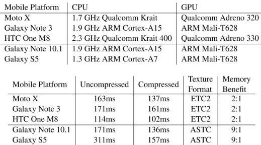
3.1 The rendering times for the polygon benchmark (Figure 3.9) from Skia using both compressed and uncompressed texturing on a variety of CPU/GPU combinations. The polygon benchmark generates a large sequence of thin, concave polygons and stores them as piece-wise 2D paths on the GPU. These polygons are then both stroked and filled to generate a large amount of paths that must be rasterized. From these results, we notice an increase in rendering speed of the heavily optimized Skia library on all mobile devices. Most importantly, the increase in memory efficiency from ETC2 (2:1 ratio) to ASTC (9:1 ratio) provides significant improvements in rendering time. These results were generated from the mean runtime of 100
executions. . . 33 4.1 Various metrics of comparison for LFSM compressed textures using intensity
dilation versus the existing state of the art tools. All comparisons were performed using the fastest quality settings of the February 21st 2013 release of the PVRTex-Tool (Imagination, 2013). For both metrics, higher numbers indicate better quality. The above results were generated on a single 3.40GHz Intel® Core™ i7-4770 CPU running Ubuntu Linux 12.04. Images courtesy of Google Maps, Simon Fenney,
andhttp://www.spiralgraphics.biz/. . . 58 4.2 Average compression speed for various compression algorithms. We use a selection
of both low and high frequency textures. FasTC easily outperforms all of the other algorithms in terms of speed while maintaining comparible quality. Tests were
performed using a 3.0 GHz quad-core Intel Core i7 workstation. . . 76 4.3 Quanititative assessment of the compression quality for the textures presented in
Figure 4.20. . . 81 4.4 Fastest available compression speeds (including our intensity dilation for PVRTC)
for a variety of formats with similar compression ratios. . . 84 6.1 Comparison of various timings in milliseconds for different compression schemes.
We test our method against various formats rendering a set of frames from a360◦
video at 4K resolution (3584×1792) similar to motion JPEG video (Wallace, 1992). . . 121 6.2 Quantitative results of single-threaded loading of the 128 textures in Pixar (2015).
The CPU size represents the size of all textures in memory after any decoding procedure and prior to uploading to the GPU. The disk bandwidth is sufficiently
fast to make decoding textures the bottleneck. . . 122
LIST OF FIGURES
1.1 An example of artifacts caused by lossy compression formats used in modern GPUs. ASTC (Nystad et al., 2012) compressesN×M blocks of pixels down to a fixed number of bits across all block sizes. The larger the blocks, the smaller the resulting texture, and the more information needs to be compressed, leading to increasingly more objectionable blocky artifacts (most noticable in the corners of
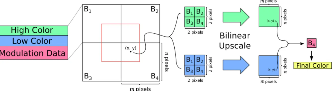
the image). . . 3 2.1 Representation of low-frequency signal modulated texture data (Fenney, 2003).
The compressed data is stored in blocks that contain two colors, high and low, along with modulation data for each texel within the block. When looking up the color value for texel at location(x, y), information is used from the blocks whose centers are the four corners of a rectangle that encompass the texel. The high and low colors are separately used to generate two block sized images using bilinear interpolation, and then the modulation value of the texel’s corresponding block is
used in conjunction with these upscaled images in order to produce the final color. . . 14
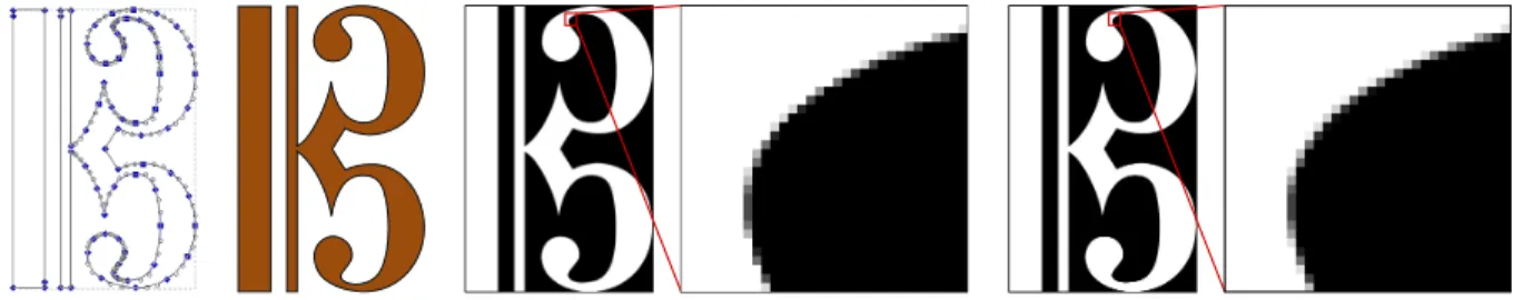
3.1 (left)The piece-wise anti-aliased cubic curve used as input.(middle-left)The final rendered curve.(middle-right)The uncompressed coverage mask passed to the GPU to determine the amount each pixel is covered by the curve. (right)The compressed coverage mask using our method. On the far right is a zoomed in comparison of the compressed and uncompressed masks. Although only a few pixels differ, using our method, these masks are compressed in real time and save
time and memory during the rasterization of these curves. . . 20 3.2 A piece-wise quadratic curve is filled with green using the Loop-Blinn method.
The pixels (pink) whose centers are not covered by the triangles circumscribing the curve will not be drawn if the GPU is not using a hardware anti-aliasing method. For power constrained GPUs, such as those on mobile devices, MSAA is prohibitively expensive due to the large number of fragment shader invocations. When the curve is non-convex, it is often more correct to default to software
rendering of the pixel coverage in these situations. . . 22 3.3 The different stages in GPU-based rendering of filled 2D regions using coverage
masks. The only part that takes place on the GPU is the compositing. Our contribution in this modified pipelineis the stage outlined in red, where compressed textures are generated directly from the run-length encoded coverage information. In doing so, we avoid both writing a full resolution texture into CPU memory and
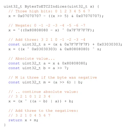
uploading a full resolution texture to GPU memory, providing savings on both ends. . . 23 3.4 C code for converting an integer storing four 8-bit values into four three-bit indices
corresponding to the proper layout of a DXTn block. Using branchless code without multiplies or divides yields extremely fast and pipelined code on modern
3.5 C code for converting an integer storing four 8-bit values into four three-bit indices corresponding to the proper layout of an ETC2 block. Similar to Figure 3.4, we perform the conversion using only bitwise operations and without expensive
multiplies or divides. . . 26 3.6 Sparse run length encoded (RLE) buffers. These buffers are used to store the
coverage information for a row of pixels prior to writing them into the coverage mask. For each pixel row, the RLE buffer is allocated to contain as many RLE entries as there are pixels. The scan converter operates on rows of super-sampled pixels, shown here as a4×4grid within each pixel, and updates the corresponding RLE buffer. In this figure, the blue entries contain the number of runs of the corresponding pixel value. Grey entries are uninitialized and never written to nor read. Samples which contribute to the coverage of the red curve are drawn in blue
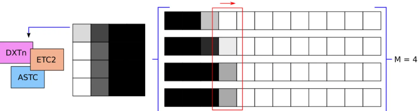
and samples that are uncovered are drawn in black. . . 30 3.7 Our scan conversion pipeline augmented to output GPU-compressed blocks. For
M×M compressed block sizes, our pipeline operates onM sparse RLE buffers in parallel (Figure 3.6). OnceM columns are processed, they are compressed into the target compressed format. For a given column, we read from the entries in the associated sparse RLE buffers. If any of the row values have changed, we update the corresponding pixel for the current column (outlined in red). Otherwise, we simply copy the previous column. For 8-bit coverage values and 4x4 compressed
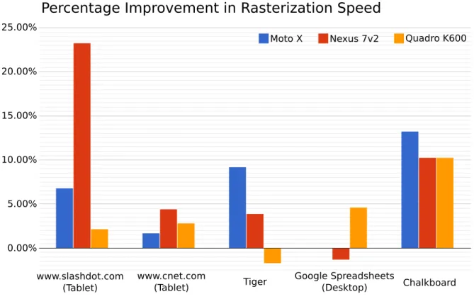
block sizes, each column fits in a single 32-bit register. . . 31 3.8 Performance improvements using compressed textures on a variety of different
benchmarks. Two of the tests performed were on tablet versions of popular websites. The Google Spreadsheets benchmark data was gathered from the desktop version of the site using many stroked paths. The other two were the vector images
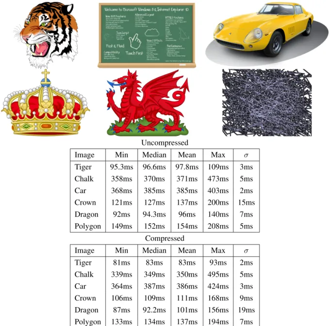
in Figure 3.9. . . 32 3.9 Rendering times of the following images on a first generation Moto X (1.7 GHz
Qualcomm Krait, Qualcomm Adreno 320) from 100 runs. From left to right the
images are labeled Tiger, Chalk, Car, Crown, Dragon, Polygon. . . 39 3.10 Detailed analysis of correctness tests within Skia most heavily affected by changes
to anti-aliased non-convex path rendering. From top to bottom, the images are labeled as ’dashed’, ’rounded’, ’poly’, ’text’, and ’strokep’. We observe very few artifacts due to compression. Although the pixels along the anti-aliased edges in the rendered images do contain different pixel values contributing to the relatively low PSNR values, the detail in the edges remains. Pixels in the difference image are on if the shaded values in the corresponding original and compressed images differ. Most noticeable in ’strokep’, the low detail of the coverage masks causes
pixel differences only in those along the edges of the filled paths. . . 40
3.11 Quantization error when converting the incoming number of samples covered per pixel to the final value stored in the compressed format. We show absolute error for both DXT and ETC formats with respect to the original quantized values. For fully opaque and fully transparent pixels we have no error as designed. For intermediate values, discrepancies in error arise from the way values are quantized in adherence
to the two texture formats. . . 41 3.12 For a 12x12 ASTC block, we maximize the number of samples we store in order
to get the finest granularity of control possible over the resulting pixels. Physical limitations of the ASTC format restrict us to a 6x5 index grid stored on disk (red samples). During decompression, these indices are interpolated to each texel (blue
samples) to compute the final index used for selecting from the precomputed palette. . . 41 3.13 (Top row) Uncompressed failure cases for certain 12x12 blocks. (Bottom row)
Our ASTC compression method applied to each block. Due to the interpolation of index coordinates in ASTC blocks, certain blocks will be compressed much more poorly than others. In particular, blocks that have many uncorrelated neighboring pixels, while able to be represented using ASTC, are not particularly well suited
for our method. However, such blocks are very rare in coverage mask textures. . . 42
4.1 The Bootcamp demo from Unity3D1using uncompressed textures (top) and using textures compressed with FasTC-64 (bottom). The visual quality of the scene is only slightly altered and no visible artifacts appear. The scene uses 156 textures which were compressed in a total of 8.75 minutes by our method. The same textures are compressed by the BC7 Compressor in the NVIDIA Texture Tools in
a total of 13.27 hours. . . 44 4.2 Real-time texture compression using intensity dilation applied to typical images
used in GIS applications such as Google Maps. Each of these 256x256 textures was compressed in about 20ms on a single Intel® Core™ i7-4770 CPU. In each pair of images, the original texture is on the left, and the compressed version is on the right. A zoomed in version of the detailed areas is given on the right. Images
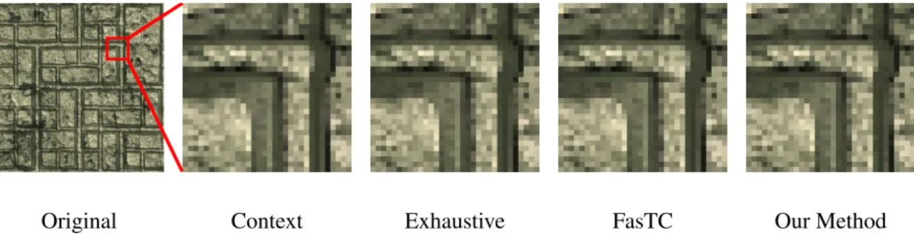
retreived from Google Maps. . . 45 4.3 Our partition-based texture compression algorithm applied to a standard wall
texture. The full original texture is shown on the far left, followed by a zoomed in investigation of the region outlined in red. Our method compresses the texture into the BPTC format. The resulting image quality, measured in Figure 4.20, is comparable to prior methods. This texture is256×256pixels large and was compressed using an exhaustive method (64 seconds (Donovan, 2010)), FasTC (567 milliseconds (Krajcevski et al., 2013)), and our method (143 milliseconds)
4.4 The different stages of the algorithm. Original texture: the texture we are com-pressing explicitly marked with an area of interest which is depicted in the zoomed in versions. Intensity: original image and zoomed in region in grayscale. Labels: labeled image and zoomed in region of texels with intensity values larger than their neighbors (green) and lower than their neighbors (blue). Forward dilation: after the first pass of the algorithm, both the high image containing local intensity maxima (top) and the low image containing local intensity minima (bottom) have been dilated forward. Backward dilation: after the second pass of the algorithm, both of the images have been completely dilated. High/Low image generation: Downscaled images that resulted from averaging all of the texels in a block of the dilated images. Modulation: computed optimal modulation values for the original image and the zoomed in region, given the computed high and low images. Final compressed texture: The resulting compressed texture and the corresponding
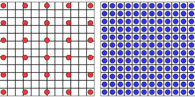
zoomed in region. Original image retreived from Google Maps. . . 51 4.5 A red and blue texture is compressed using LFSM compression. Green positions
are block centers. Since the border between blue and red areas aligns with block borders, the optimal compression is to store one color as the high color of each block, and another color as the low color of each block. The modulation data is
used to reconstruct the original image. . . 52 4.6 Examples of dilation. Left: a red star is dilated by a smaller circle into the green
star with rounded corners. Right: Two pixels, denoted in green, are dilated three times using a3×3pixel box. If an empty pixelpis to be filled during dilation from multiple pixelsqiof different values, then the value stored forpwill be the
average of theqi. The picture is labeled with the values that the pixels would take
after dilation of the initial pixels. The pixels that have fractional labels denote the
value that they would have taken between labels one and two. . . 54 4.7 Our fast approximate dilation strategy. We perform the extrema calculation and
dilation in two passes. Top Left: First pass, traverse the pixels from left to right, top to bottom labeling and dilating extrema in the order of traversal as we encounter them. Top right, bottom left, bottom right: Second pass, traverse the pixels from right to left, bottom to top. At each pixel, assign the label corresponding to the
average of the pixels with the lowest distance to their respective labels. . . 55 4.8 Problems with using PSNR as the only metric. Each image above has a similar
PSNR to the original image on the far left. Images courtesy of Wang et al. (2004). . . 57 4.9 Investigation of areas with high detail in some common mobile graphics
im-ages. We notice that the texture compressed using intensity dilation maintains the smoothness of many image features, while the original PCA based approach leaves blocky streaks. Images courtesy of Google Maps, Simon Fenney, and
http://www.spiralgraphics.biz/. . . 59
4.10 Detailed investigation of areas with high pixel homogeneity. Unlike the images in Figure 4.9, we notice that the texture compressed using intensity dilation suffers from artifacts arising from aggressive averaging of nearby intensity values, while the PCA based approach has relatively good quality compression results. Original
image retreived from Google Maps. . . 61 4.11 (right)A 4×4 block of texels.(left)The texels approximated with two-bit indices.
The texels are interpreted as points on a lattice defined by the precision of the source texture (red). The endpoints approximating the texels are on a sparse lattice (blue) and the interpolation points are in green. For two bits per index we have 22 = 4interpolation points. Note: The internal interpolation points do not lie on
the line segment due to quantization. . . 62 4.12 A 4×4 block partitioned by different P-shapes into two subsets from the BPTC
format. P-shape partitioning is determined based on a lookup into a table of common partitionings. The texels marked with a pink background belong to one subset and the unmarked texels belong to another. Each subset is approximated
with its own line segment (in green).(left)P-Shape #31(right)P-Shape #4 . . . 64 4.13 Overview of FasTC which is applicable to all endpoint based compression formats
that support partitioning. . . 64 4.14 An overview of the SegTC compression algorithm. (a) The VP-Tree is constructed
from format-specific P-shapes as a preprocessing step. (b) For each image, we perform SLIC segmentation. For each block, we extract the corresponding par-titioning that matches the superpixel boundaries and find the nearest P-shapes using the VP-Tree. The closest P-shapes are used with the cluster-fit algorithm to
produce the final compression parameters. . . 68 4.15 (left) The original image. (center) An investigation of the area highlighted in teal.
(right) SLIC superpixels: the image is segmented into small regions that adhere to
feature boundaries (Achanta et al., 2010). . . 69 4.16 Peak Signal to Noise Ratio for various compression algorithms. NVTC, the
tool provided with NVIDIA’s Texture Tools (green). FasTC-0, our algorithm without simulated annealing (blue). DX CPU, the tool provided with Microsoft’s DirectX SDK (red). Our algorithm (FasTC-0) provides similar quality to existing
implementations. . . 77 4.17 Detailed investigation of areas with high noise in the Kodak Test Images that
produce lowest PSNR. We notice that the visual quality of FasTC is comparable to
NVTC and close to the original texture. . . 78 4.18 Peak Signal to Noise Ratio for FasTC-0 using bounding box estimation (blue)
and eigenvalue comparison (red). In this experiment, we replaced the shape estimation technique from FasTC-0 with one that uses the ratio of the first and second eigenvalues of the covariance matrix. We can see that due to quantization
4.19 We compare the compression quality of the original NVTC (green) with a modified version that measures shape quality using bounding box estimation (red). In general, the difference in PSNR is very small, but we avoid a costly eigenvector
computation during shape estimation giving us up to 10x in performance gains. . . 79 4.20 From top to bottom we compare encodings of ’satellite’, ’colorsheep’, ’pebbles’,
and ’crate’. To complement our segmentation algorithm we have chosen a repre-sentative sample of textures that are meant to be consumed visually, and report errors using both peak signal-to-noise ratio and the structural similarity image metric. Additionally, we notice that the choice of segmentation is very important because we lose some detail in parts of ’colorsheep’ where the segmentation is too large to catch fine details. To contrast, we maintain the visual detail of ’pebbles’ and ’satellite’ very well. The texture ’colorsheep’ is provided courtesy of Trinket Studios, Inc. The texture ’satellite’ is provided courtesy of Google, Inc. The
remaining textures are public domain fromwww.opengameart.org. . . 80 4.21 The run-time of SegTC against FasTC. Images used are labeled in Figure 4.20
’brick’ refers to the texture displayed in Figure 4.3. The exhaustive algorithm is not displayed in the performance graph because it is two orders of magnitude slower than FasTC. We observe an increase in encoding speed over existing implemen-tations while maintaining a similar quality level. All timings are performed on a
single core Intel Core i7-4770 CPU 3.40GHz without vector instructions. . . 81 4.22 Average compression speed in seconds of the images in the Kodak Test Image suite
for various different amounts of simulated annealing (FasTC-0 to FasTC-256). Since a constant amount of simulated annealing is applied once for each texel block, the increase in compression speed is linear. Tests were performed using a
3.0 GHz quad-core Intel Core i7 workstation. . . 82 4.23 Average increase in Peak Signal to Noise ratio for the images in the Kodak Test
Image suite for various different amounts of simulated annealing. The increase in
quality is sublinear due to the nature of the solution space. . . 83 4.24 Compression time in seconds for FasTC-0 of a20482 sized texture on different
multi-core configurations using different numbers of threads. Tests were run on a Single-Core 3.00 GHz Pentium 4 running 32-bit Ubuntu Linux 11.10 (red), Quad-Core 3.50 GHz Intel Core i7 running 64-bit Windows 7 (blue) and 40-Core 2.40 GHz Intel Xeon running 64-bit Ubuntu Linux 11.04 (green). We observe a
linear speedup with the number of cores. . . 84 5.1 Demonstration of the subdivision of the Samsung logo. The constant color regions
of the texture are low in detail and can accurately be approximated using12×12 blocks while the blocks along the edges are subdivided to provide additional detail. For4×4metadata, we can reuse the low-detail12×12blocks by referencing them in the low-detail4×4and8×8blocks. The subdivision visualization colors
match those in Figure 5.2. . . 89
5.2 The seven different configurations of a12×12ASTC block. It can be subdivided into four6×6blocks, nine4×4blocks, or any one of four different ways to store
a single8×8block and five4×4blocks. . . 91 5.3 (Top Row) Seven12×12blocks compressed adaptively and packed on disk using
the same color scheme as Figure 5.2. (Bottom Row) The same seven blocks expanded out to cache-line granularity to decrease the number of cache lines
required to access an entire12×12block. . . 92 5.4 Texture fetch flow in a traditional fixed-rate pipeline (top), and our proposed
variable bit-rate method (bottom). Note that the block address generation step in a traditional pipeline – a function of the texel format and memory layout – is now
replaced by a metadata table lookup . . . 93 5.5 Block distribution with (left) 4x4 metadata and (right) 12x12 metadata. Comparing
these results to Figure 5.10, we observe that higher percentages of12×12blocks
leads to higher compression rates. . . 99 5.6 Images with which our algorithm performs relatively poorly. In these images
tuning the local subdivision criteria proves difficult. We observe this in images that have uniform low detail with noise, such as bump maps. For comparison with ASTC, we observed (left) 43.8 PNSR (8 bpp) against 40.8 PSNR (9 bpp) with adaptive 4x4 metadata, (middle) 55.27 PSNR (8 bpp) against 40.4 PSNR (7.58 bpp) with adaptive 12x12 metadata, and (right) 39.43 PSNR (5.12 bpp) against
32.94 PSNR (6.32 bpp) with adaptive 4x4 metadata . . . 99 5.7 Percentage of unique blocks in the four sample color images from Figure 5.10.
We show results for both4×4and12×12metadata. Higer values indicate more
unique detail and correlates with larger bitrates for the final compressed texture. . . 100 5.8 A comparison of different compression algorithms. (top) We select a few images to
compare PSNR against compression size measured in bits per pixel. We compare against ASTC, JPEG2000 (J2K) and Olano et. al. (Olano et al., 2011). The designationsv1,v2andv3are used to match those presented in the paper (Olano et al., 2011). (middle) The same comparison across all images from the Kodak Test Image Suite(KODAK, 1999). (bottom-left) Comparison of MSSIM(Wang et al., 2004) across the Kodak images. (bottom-right) Comparison of cache coherency measured in total cache misses for hardware formats. As we can see from these results, our algorithm performs favorably on images with non-uniform distribution of details. We can contrast the natural images from the KODAK Image Suite against theandroidimage from Figure 5.10, where our adaptive12×12variant performs significantly better than ASTC approaching bitrates similar to J2K. Furthermore, we can observe the effect of the metadata overhead in our approach with some images with a larger bitrate than4×4ASTC. From the cache coherency graph, we can see that for certain images, we are within the same number of cache
5.9 Similar to Figure 5.8, we compare a large suite of images with bitrate versus PSNR. The images used were from the Kodak Image Suite(KODAK, 1999), the 128 Pixar Textures(Pixar, 2015), the Retargetme Image Suite(Rubinstein et al., 2010), and the images from Figure 5.10. In this plot, we notice many of the images here are high detail bump and normal maps, for which our algorithm performs poorly. These images usually contain very uniform detail and require accurate compression. Our method subdivides these images to full4×4ASTC, creating clusters around at 9.5 bits per pixel for4×4metadata and 8.1 for12×12metadata. Similarly, for some images, such as those in the lower-left portion of the plot, their high repetitive nature or large areas of low detail make them ideal candidates for our method. Additionally, we observe a significant difference between non-GPU based variable bitrate algorithms. In particular, J2K has a much more tunable
quality threshold that is apparent in the bitrate distributions of images. . . 102 5.12 grandcanyon . . . 102 5.10 An analysis of our method for compressing textures against Adaptive Scalable
Texture Compression (Nystad et al., 2012). We observe that sparse textures, such as alto and android, take advantage of the redundancy inherent in dictionary encoding and produce significant gains. A variety of metrics using ARM (2012) are included. In our adaptive compression schemes we require the error for each grayscale block to be within||∆B||∞ <4and each color block to be within||∆B||∞ <8. We
compare the compression quality per bit per pixel and the number of times we would miss an 1KB L1 cache with 64B cache lines for raster and morton access
patterns. . . 103 5.11 A comparison of the compression artifacts generated by each algorithm. We
compare our method against Adaptive Scalable Texture Compression (Nystad et al., 2012). As in Figure Figure 5.10, our adaptive compression schemes require the error for each grayscale block to be within||∆B||∞<4and each color block
to be within||∆B||∞<8. . . 104
6.1 The constituent parts of a compressed texture. Each endpoint compressed texture represents a sequence of equally sized blocks. Each block contains a fixed number of bits containing two endpoint colors that generate a palette and per-pixel index data. Here we show the endpoints separated into individual images and visualize the per-pixel indices. We re-encode the indices using VQ-style dictionary com-pression and transform the endpoint images using a wavelet transform prior to
encoding the final texture using an entropy encoder. . . 109 6.2 The first stage of our encoding pipeline. We process each block in raster-scan order
while maintaining a dictionary of recently added index blocks. For each index block, if we find an existing index block in the dictionary that closely matches the original, we reuse that index block. If significant error is introduced, then we add
this index block to the dictionary. . . 110
6.3 Our decompression pipeline. Pink boxes represent separate GPGPU executions for which red arrows are inputs and the blue arrows are the outputs. Per our design, the supercompressed texture data can be uploaded directly to the GPU for decoding. The input data and intermediate results all remain resident in GPU memory during decoding. Multiple texture streams can be interleaved between the symbol frequencies and the ANS streams to provide additional decoding
parallelism. . . 116 6.4 The affect of varying the number of symbols per decoding thread, and hence
number of parallel decoders, as a comparison between average file size and de-coding time of 600 frames of a 4K360◦video. When decoding few symbols per thread, size is dominated by storing many encoder states, although the increased parallelism helps decoding speed. Copying the ANS decoding table (Section 6.2) into local memory only benefits decoding speed when there is enough work per
thread to benefit from fewer global reads. . . 121 6.5 The difference in PSNR and compression size as a function of our error threshold
for a few images from the Kodak test suite. As we increase our error threshold, we see a decrease in the size of our index data and a drop in our PSNR. Both of these metrics are sensitive based on the features of the encoded image. The PSNR stabilization after an increase in the error threshold supports the assumption of
block-level coherency between indices. . . 122 6.6 We show PSNR versus bitrate values for our method against other compression
schemes. The data shows that our method provides bit rates and quality comparable to the state of the art supercompressed textures. Each data point is an image in the (top) KODAK (1999) and (bottom) Pixar (2015) datasets with dimensions
512×512. . . 123 6.7 We demonstrate a comparison of the compressibility of various approaches to
preprocessing index data. This graph demonstrates the size of the compressed index data for various algorithms against KODAK (1999) using the same Huffman encoder used in the Crunch textures. Palette indices are classically the most incoherent data in compressed textures. We show that by limiting the dictionary lookup to thekmost recently added dictionary entries, we increase the entropy encoding capabilities of the index data significantly over Crunch at maximum quality settings. Compressed raw is Huffman encoding applied to the unprocessed index data while the predicted method is the same method used by Str¨om and
Wennersten (2011) applied to DXT textures. . . 124 6.8 A zoomed-in view of the visual quality of various compressed formats. The only
stage in our compression pipeline that may introduce additional error is the re-encoding stage. Here we show that the amount of error introduced is imperceptible
with respect to other DXT compression formats. . . 124 6.9 An average of the percentage-wise breakdown of each of the constituent parts of a
GST encoded texture using various error thresholds. As we allow more error, the size of the dictionary decreases as a percentage of overall space consumed. We
7.1 A Z-order curve at different resolutions. Each increased resolution follows a
similar structure from the previous resolution. Image courtesy of David Eppstein. . . 131 7.2 (left) The current GPU programming model with respect to texture accesses.
(right) The proposed GPU programming model where texel values are generated by running small programs as part of the texture pipeline. Each GPU program (compute) that runs may make one or more memory requests (outlined) from different memory types usually handled in parallel. During each memory request, GPU programs are preempted to allow other parallel work to execute. As a result, the proposed architecture changes would be to allow an additional program to compute the texel samples needed as a part of each texture access. These programs would be free to make their own memory requests in order to compute the final pixel values. Each of the other existing caching mechanisms would remain in place, allowing the programmer to make a choice between optimizing caching
behavior and compressed texture size. . . 133
LIST OF ABBREVIATIONS
Texture Compression Formats:
S3TC S3 Texture Compression (also known as DXT and BC1) PVRTC PowerVR Texture Compression
BPTC Block Partitioned Texture Compression (also known as BC7 and BC6H) ETC Ericsson Texture Compression v1
ETC2 Ericsson Texture Compression v2 ASTC Adaptive Scalable Texture Compression S3TC S3 Texture Compression (also known as S3TC)
BCx Block Compression as defined in the Microsoft DirectX specification VBR Variable Bit Rate Compression
GST GPU-Decodable Supercompressed Textures
Image Similarity Metrics:
PSNR Peak Signal to Noise Ratio
SSIM Structural Similarity Image Metric
Other Compression Formats:
JPEG Joint Photographic Experts Group PNG Portable Network Graphics
DPCM Differential Pulse Code Modulation ANS Asymmetric Numeral Systems
Miscellaneous:
CHAPTER 1: INTRODUCTION
Over the past three decades, computer graphics has matured into a robust and well-studied field. With our understanding of the physics of light and display technology, synthesized images are becoming increasingly indistinguishable from photographs. As with most aspects of modern computing, we are limited by available resources such as processor speed and memory size for each generated frame of animation. In the extreme, interactive graphics applications limit the amount of computation for a given frame to the time in between display updates, typically 16 milliseconds which allows for 59.94 frames per second on modern high definition displays. To facilitate this performance, dedicated hardware, or graphics processing units (GPUs), are used to perform large batches of computations in parallel.
One of the main uses of GPUs is to determine the visual appearance of a given set of geometric primitives on a modern display. Although many different rendering techniques have been proposed in the literature, modern hardware has been optimized for the processing and display of triangles. Many algorithms governing modern GPU architecture roughly correlate rendering performance to the number of triangles drawn in a given frame. To maintain performance, large triangles are generally used in order to better exploit the benefits of the parallelization of modern GPUs. In order to preserve the detail on these triangles,texture mappingis a technique that parametrically maps images (textures) onto triangle surfaces (Catmull, 1974). This technique has become so prevalent that GPUs have specialized hardware for storing and accessing textures to boost overall performance.
storage device, such as a hard disk or the network, to main memory for use with the CPU, and finally to the video memory on the GPU. Even traditional personal computers are limited by the amount of data that can be transferred. Additionally, certain architectures such as the systems-on-a-chip used in mobile devices are much more sensitive to power consumption and memory bandwidth restrictions (Imagination, 2016). A significant amount of this overhead is inherent in accessing the texture data stored in memory during rendering (Nixon et al., 2014).
Recent advances in graphics hardware have pushed for compact representations of texture data. These compressed data techniques either provide additional cost savings by requiring less memory for texture storage on disk, or increase the visual quality of interactive graphics applications by allowing more detailed textures to be used. Additionally, the smaller size of textures provides faster load times from the disk or network into CPU RAM and from CPU RAM into GPU RAM. The number of memory accesses needed during rendering is also reduced due to the amount of data contained in a smaller chunk of memory. The ability to leverage these representations becomes a boon to application developers and providing this accessability is very important problem.
1.1 Texture Compression
Over the past half-century, there has been significant research in image compression algorithms (Duce, 2003; Wallace, 1992; Skodras et al., 2001). However, in order to render these images, they must be decompressed in order to get access to the raw pixel values. These pixels are usually represented using a value in the range[0,255]for each red, green, and blue channel to correspond to the underlying structure of modern displays. An optional alpha channel may be used for transparency. This corresponds to24or 32bits per pixel in a decompressed image. As an example, a typical image without alpha of dimensions 768×512is1.18MB in memory. Using JPEG compression, this image can be stored using only128KB, approximately a 10X savings.
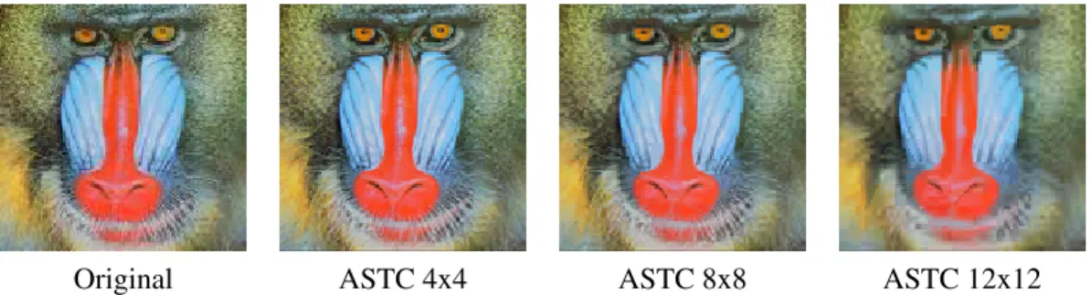
Original ASTC 4x4 ASTC 8x8 ASTC 12x12
Figure 1.1: An example of artifacts caused by lossy compression formats used in modern GPUs. ASTC (Nystad et al., 2012) compressesN ×Mblocks of pixels down to a fixed number of bits across all block sizes. The larger the blocks, the smaller the resulting texture, and the more information needs to be compressed, leading to increasingly more objectionable blocky artifacts (most noticable in the corners of the image).
preservesrandom accessto the pixels. In other words, for any given pixel at location(x, y)in the image, the compressed respresentation specifies a functionf :Z2 →Zthat maps this location to a sequence of
bits shorter than the original pixel representations. These bits are read by the graphics hardware and sent through fixed-function decoding units to produce resuling pixel values.
Texture compression allows textures to be represented in a compact representation during transfer from the CPU to the GPU, although they are not as efficient in compressing textures for disk or network storage. The dedicated GPU decoding hardware facilitates rendering by providing fast access to pixel values directly from the compressed format. However, these random access requirements restrict the total compressibility of the textures. Certain image compression algorithms such as JPEG are able to exploit redundancies across neighboring pixels to reduce the amount of bits required to represent low-detail regions. The more redundancy there is in the pixel values, the more that can fit within a given amount of memory, such as a low-level memory cache. A hardware decoder for such a format would require multiple memory accesses that are expensive in terms of both power and latency (Nixon et al., 2014). Although these limitations may be inconsequential for a certain class of images as described in Chapter 4.3.3, compressed textures represent a fixed number of pixels using a fixed number of bits. This creates a dichotomy where solid colors are ’compressed’ using the same number of bits as random noise. With only one memory lookup, to achieve any amount of compression, these formats must be lossy in order to target the common use case rather than the worst-case. As shown in Figure 1.1, the result is often a trade-off between size and data loss that dominates the design of these compression formats.
1.2 Encoding Compressed Textures
Compressed textures are typically stored by having fixed-size blocks of pixels compressed down to a fixed number of bits. The block dimensions are usually chosen to be roughly square in order to map well to access patterns during rendering. In other words, if the GPU requests a certain pixel to render from a texture, there is a high chance a neighboring pixel will be requested as well. This block structure, combined with the overall variability of image intensity values contained in a block, presents a difficult problem for the compressor. The fixed size of the compressed representation implies a significantly smaller set of blocks that can be represented exactly. Hence, the compressor must choose the compressed representation whose reconstructed block of pixels most closely matches the original block. As an example, suppose a compression format encodes4×4blocks of pixels as64bits. At24bits per pixel, this structure implies2384total possible blocks are restricted to264possible compressed representations. In order to choose the proper compressed representation for a given block of pixels, texture com-pressors typically are incapable of using an exhaustive method. In the previous example, there are approximately1.84×1019 possible valuesper-block. For a1024×1024texture, this implies more possible values than molecules in a typical glass of water! Hence, most algorithms tend to approximate the best compressed representation per-block by using ad-hoc approaches with various heuristics that map well to the given representation.
Because compressed representations are designed for fast decompression, slow compression times were originally acceptable (Beers et al., 1996). However, in recent years, the amount of texture data used in interactive graphics applications has exploded. In particular, mobile UIs are increasingly being driven by GPUs requiring many re-loads of texture data (Google, 2016). For this reason, many of the billions of photographs taken each day and uploaded to social media sites such as Facebook and Twitter may need to be compressed into formats amenable to rendering on the GPU. Current game engines spend up to 80% of their asset processing time on compression of raw texture data (Chen, 2016). In order for application developers and texture artists to properly iterate over their data, compression algorithms must be relatively fast. Otherwise, optimizing for proper compression ends up causing significant bottlenecks in the overall application development pipeline.
colors, known asendpoints, are used to create a palette with2bcolors using linear interpolation in color space. The additionalbbits per pixel are then used as paletteindicesfor selecting the pixel color for each block. An encoder is then tasked to determine both endpoints and indices for each input block of pixels. To vary the amount of detail in the final representation, the number of bits allotted to each endpoint and index is usually variable across compression formats.
Recent formats have expanded this basic idea to give additional detail. Some formats bilinearly interpolate the palette endpoints across blocks during decompression to give specialized per-pixel endpoints (Fenney, 2003). Others partition the block into multiple different subsets of palettes (OpenGL, 2010; Nystad et al., 2012). Due to the large number of possible partitionings, most formats limit the number of available partitions to a subset that provide the most benefit to common image features. Each of these different features creates additional complexity to the encoders that determine the final compressed representation. In particular, choosing a particular partitioning of a block to preserve the most detail is usually the most time consuming component of any encoder (Krajcevski et al., 2013).
1.3 Thesis Statement
The performance and development of interactive graphics applications can be improved through
the fast computation of compressed texture representations that are either decoded or used directly with
existing graphics hardware.
This statement reflects a variety of improvements developed to better facilitate the use of compressed textures from the perspective of application developers. In general, we aim to investigate the main performance bottlenecks of common encoding algorithms and eliminate them by relaxing the constraints on the search space of possible encodings. With the fast encoding algorithms, we also show that current texture compression algorithms can be improved in terms of storage space by providing additional features to target images with mixed amounts of detail. Finally, we show that the disk storage of these compressed formats can be improved by using an additional layer of compression that is amenable to fast decompression on the GPU.
1.4 Main Results
The main focus of this dissertation is to discuss how faster encoding algorithms lead to a variety of improvements for compressed textures. By developing accelerated methods for compressing textures, we can use the encoders to investigate benefits of other compressed texture methods, and use ’optimal’ encodings as baselines for introducing additional error. By having this baseline, we can quickly determine the implications of making changes and additions to new compression methods and quickly determine their efficacy.
1.4.1 Accelerated Texture Compression
The first algorithm focuses on the general problem of encoding low frequency signal-modulated (LFSM) compressed textures such as PVRTC (Fenney, 2003). This method bilinearly interpolates the per-block endpoints in order to generate per-pixel endpoints defining a palette to choose from. This bilinear interpolation implies that an endpoint stored in a4×4block influences the final color of a7×7 block of pixels. To search for these endpoints, we find the local minimum and maximum intensity values in this7×7block and average them. Using this technique, textures can be encoded into LFSM formats at 3X the speed of prior compression algorithms without any significant loss in quality, as described in Section 4.1.
More recent formats, such as BPTC and ASTC, have much more complicated compressed rep-resentations. These formats define a way to choose from a set of predefined block partitionings that provide separate palettes for each subset of pixels (OpenGL, 2010; Nystad et al., 2012). Prior state of the art encoders would use an exhaustive search of each of the available partitionings. This exhaustive search amplifies the already difficult problem of finding a proper palette for a given set of pixels as it requires a separate palette search for each possible subset. Approximations to the appropriate palettes for given partitionings provide similar results to doing a full search with respect to PSNR. These approxi-mations, taken from real-time texture encoding algorithms, provide orders of magnitude speed-ups for partition-based compression formats as described in Section 4.2.2.
by performing a global segmentation of image features. The boundaries of each segmentation label define the ’optimal’ partition subset boundaries in a given block. The available partitioning closest to the ’optimal’ choice can then be used to represent the block. Furthermore, all available blocks can be preprocessed into a VP-tree forO(logn) query given an ’optimal’ block. This method provides an additional 3X speedup over prior methods as described in Section 4.2.3.
1.4.2 Applications of Interactive Compression Algorithms
In the extreme case, real-time compression algorithms can be used as an intermediate step in common rendering tasks. In particular, textures that are generated on-the-fly may benefit from real-time texture compression if the encoding is performed fast enough that the gains from uploading a smaller texture can be realized. To do this, the approach must be application-specific and tailored to the compressed format. These benefits are realized even more on mobile devices where the CPU-GPU bandwidth limitations are even greater.
One application that we investigate is the generation of coverage information in GPU-based 2D renderers. Coverage information is the per-pixel value that describes how much that pixel is covered by rendered geometric primitives. For certain primitives, such as lines, triangles, and points, these values can be analytically derived on the GPU. However, for other primitives, such as closed-loop quadratic and cubic curves that are used as the basis for many font representations, the computation may be much more difficult. To deal with this problem, some GPU-based renderers compute the coverage information using a traditional CPU rendering approach. The subsequentcoverage maskis stored in a texture and uploaded directly to the GPU for rendering. To accelerate this process, the coverage mask can be generated directly into a compressed format circumventing both the full CPU write and the CPU-GPU bandwidth. Our method gives up to a 2X speedup over traditional GPU-based methods on certain benchmarks and up to a 9:1 savings in GPU memory as shown in Chapter 2.6.
1.4.3 Storage of Modern Compression Formats
Although texture compression formats are fixed-rate, recent formats allow variable global block sizes giving application developers a size versus compression quality trade-off. Different block sizes can be decoded in hardware by the same functional unit, effectively reducing the amount of different formats needed on a GPU. However, this limitation still implies a global fixed compression size for a
given texture. Hence, low-detail areas and high-detail areas will not have different levels of compression. By adding a single additional memory lookup, we can dynamically choose the compressed block size for a given set of pixels. In this way, we present a method for variable bit-rate compressed textures that requires a very small addition to the addressing unit of hardware decoders. In Chapter 4.3.3, we reduce the storage size of certain textures by up to 2X while maintaining acceptable compression quality.
In addition to memory storage, the disk storage of compressed textures is critical to the overall performance of interactive graphics applications. Loading textures from disk is usually more time consuming than uploading them to the GPU. However, texture compression formats are still about four times larger than image compression formats on disk. This becomes an even bigger problem for textures that are used with GPU-driven user interfaces or for applications that request texture data over the network, as image databases are growing at unprecedented rates. In order to address this issue, the endpoints and indices of compressed textures can be stored and processed independently. In particular, endpoints are treated as low resolution images and stored with image compression techniques while indices are approximated using a common dictionary. Along with a GPU-enabled decoding scheme, compressed textures can be stored on disk and uploaded all the way to the GPU for decoding, saving both CPU-GPU bandwidth and disk storage while maintaining acceptable compressed quality, as described in Chapter 5.4.
1.5 Thesis Organization
features could be added moving forward to provide additional benefits and flexibility are discussed in Chapter 6.5. Conclusions and final remarks are given in Chapter 7.5.
CHAPTER 2: TEXTURE COMPRESSION VERSUS IMAGE COMPRESSION
Traditional image compression algorithms such as PNG and JPEG assign bits to pixels with respect to the amount of detail in an image. In other words, images that contain many common pixels or contain neighborhoods of similar pixels require fewer bits in the final encoding. Hence, traditional image compression offersvariable-ratecompression depending on the details of the image. Often, in order to remove some redundant detail, the raw RGB values usually undergo one or more transforms. For example, JPEG uses the discrete cosine transform to condense the information content of blocks of pixels (Wallace, 1992), and its successor, JPEG-2000, uses one of two wavelet transforms depending on whether or not lossless encoding is desired (Skodras et al., 2001). Similarly, colors are usually transformed into color spaces that condense information into a single channel in order to increase overall compression efficiency. One such example is the lossless conversion of 8-bit RGB to a colorspace such as YCoCg (Malvar et al., 2008).
Given analphabetofsymbols,entropy encodingis the practice of converting a sequence of symbols into a sequence of bits by assigning bits to symbols based on the probability of each individual symbol appearing in the given sequence. Entropy encoding techniques, such as Huffman (1952), arithmetic (Ris-sanen and Langdon, 1979), and ANS (Duda, 2013) encoding are the basis for many image compression formats (Buccigrossi and Simoncelli, 1999). Without additional metadata, the variable number of bits per symbol forces serial decoding algorithms for any given encoding algorithm. A variable number of bits per encoded symbol requires all previous symbols to be decoded prior to any specific symbol, although some attempts have been made to increase the scalability of these techniques to multiple processors (Klein and Wiseman, 2003; Kim and Park, 2007).
rate formats, the current state-of-the-art compression formats, and a few notes on the methods for deriving the compressed representation from a given input image.
2.1 Fixed Rate Image Compression
The origin of most fixed rate formats follow the format of a technique known asVector Quantization (VQ). This technique, originally used in signal processing, represents a sequence of n values (or codewords) by storing a dictionary of sizek < nand replacing each codeword with the appropriate index into the dictionary. Lossless compression using VQ can actually require more data than storing the original set of codewords when all of the codewords are distinct. However, for data that does not need to be stored without loss, a few representative dictionary entries can be used to approximate each of the original codewords. If the data represents a quantity perceived by humans, such as audio or image data, then the loss may be acceptable without losing the perceived quality.
Fixed-rate texture compression formats are a variation of this technique. If a sequence of pixels originally stored inn bits is compressed down to a fixedk < n bits, we are effectively defining a dictionary of size2k. The specification of this dictionary is implicit in the decoding algorithm for the
texture once it has been compressed. In other words, since two sequences ofkbits are decoded to the same originalnbits, the ’dictionary’ is defined by the logic that does this decoding. This is counter to the original formulation of VQ in which the dictionary is stored along with thek-bit entries. Hence, the size and quality of any given compressed texture representation is specified by how well its ’dictionary’ is defined.
Today’s fixed-rate encoding schemes mostly follow the Block Truncation Coding (BTC) technique introduced by Delp and Mitchell (1979) for compressing eight-bit grayscale images. In this format, 4×4 blocks of pixels are encoded using two eight-bit grayscale values and a per-pixel bit selecting choosing one or the other. Each block is therfore compressed into two bytes offering twobits per pixel(bpp). Various generalizations of this idea have been proposed by Nasrabadi et al. (1990); Fr¨anti et al. (1994).
Campbell et al. (1986) extended the idea of BTC to include color by introducing a 256-value color palette instead of grayscale values. By specifying a single palette for the entire image, the use of eight-bit entries into this palette compresses images down to 2 bpp. However, the additional memory lookup made
it difficult to render from directly on GPUs. This method, known asColor Cell Compression(CCC) was used predominantly in the architecture presented by Knittel et al. (1996).
The random access properties of fixed-rate compression imply a lossy compression algorithm. However, texture mapping hardware can quickly compute an address to the underlying texture data. Similar to BTC and CCC, typical fixed-rate compression formats representN ×M blocks of pixels in some fixed number of bits. Many graphics architectures were proposed using similar compressed texture representations (Torborg and Kajiya, 1996; Knittel et al., 1996; Beers et al., 1996).
2.2 Graphics Architectures for Compressed Textures
Knittel et al. (1996) introduced a graphics architecture that supported compressed texture representa-tions via CCC introduced by Campbell et al. (1986). In particular, Knittel et al. (1996) describe the use of a high-throughput multi-bank memory system that could handle multiple addresses corresponding to neighboring pixel values. An additional hardware decoder was used to obtain close-to-interactive decom-pression speeds by requiring fewer bytes in memory and allowing different page table configurations. Torborg and Kajiya (1996) take a similar approach by preserving the compressed format in memory, although the details are not disclosed.
The algorithm provided by Delp and Mitchell (1979) was able to meet the necessary requirements of texture decompression hardware as described in Section 1.1, namely the need for fixed-rate addressing and an algorithm that can be implemented in hardware. Although fixed-rate compression has been used for almost three decades (Chandler et al., 1986)(Economy et al., 1987), texture compression in graphics architectures based on Vector Quantization (VQ) was formally presented by Beers et al. (1996). In this seminal paper, Beers et al. argue for four main tenets of texture compression: fast hardware decoding speed, preservation of random-access, compression rate versus visual quality, and encoding speed. The presented argument claims that encoding speed could be sacrificed for gains in the other three, but the need for fast encoding algorithms was recognized even then, where a Generalized Lloyd’s Algorithm (Gersho and Gray, 1991) was used to produce fast non-optimal encodings.
efficient pixel access. This architecture stored textures in a binary tree that allowed rendundancies in blocks to be eliminated by a clever differencing scheme. However, these methods require expensive addressing schemes and do not leverage existing compressed texture hardware. More recently, commercial mobile GPU manufacturers have support for surface or render target compression (nVidia, 2015, 2014; Imagination, 2016). A discussion of a compressed texture representation that proposes a simple addressing scheme but maintains some of these benefits is discussed in Chapter 4.3.3. As few hardware and algorithmic details are public about the proprietary architectures, it is difficult to compare the performance of commodity GPUs.
2.3 Modern Texture Compression
Along with the advent of commodity graphics hardware, a variety of texture compression formats emerged. These formats have largely fallen into two broad classes of compressed formats. The first class, known asendpointcompression formats, are extensions of the original per-block paletted formulation introduced by Delp and Mitchell (1979). The second, known astabledcompression formats, use a set of predefined tables that describe the compressed block. In this section we will discuss both formats in detail.
The basis of all endpoint compression formats are two low-precision RGBendpointsper block that generate a palette of colors by linear interpolation. Along with these two low-precision colors, a per-pixel paletteindexis stored to recreate the final pixel color, just as in the original BTC (Delp and Mitchell, 1979; Fenney, 2003; OpenGL, 2010; Nystad et al., 2012). Among the first endpoint compressed texture formats available on commodity graphics hardware was S3TC (also known as DXT and BC1), introduced by Iourcha et al. (1999). In this format,4×4blocks of pixels are represented using two16-bit values and16two-bit values. The two16-bit values are each interpreted as RGB endpoints with five bits for the red and blue channels and six bits for the green channel. These endpoints generate a four-color palette for the block via linear interpolation. The following16two-bit values index into this palette to recreate the final pixel values. Recently algorithms have been developed that provide additional quality over S3TC by either cleverly using the compression format, such as storing wavelet coefficients in the compressed texture and reconstructing pixels at run-time (Mavridis and Papaioannou, 2012), or by weighing the importance of endpoints based on the input (Krause, 2010).
High Color Low Color Modulation Data pixels m pix els n
B1 B2
B3 B4
(x, y)
B1 B2
B3 B4 2 pi
xels
2 pixels
B1 B2
B3 2 pi
xels 2 pixels B4 Bilinear Upscale n pix els mpixels (x, y) n pix els mpixels (x, y) B4 Final Color
Figure 2.1: Representation of low-frequency signal modulated texture data (Fenney, 2003). The com-pressed data is stored in blocks that contain two colors, high and low, along with modulation data for each texel within the block. When looking up the color value for texel at location(x, y), information is used from the blocks whose centers are the four corners of a rectangle that encompass the texel. The high and low colors are separately used to generate two block sized images using bilinear interpolation, and then the modulation value of the texel’s corresponding block is used in conjunction with these upscaled images in order to produce the final color.
Fenney (2003) later described decompression hardware that took advantage of the worst case of S3TC during texture filtering. In this case, the graphics hardware must generate a color by bilinearly interpolating the color between four pixels in a 2×2 square. If pixels all correspond to different blocks, four compressed block lookups need to be performed regardless. In his approach, known as Low Frequency Signal Modulated Texture Compression (LFSM), the RGB endpoints of neighboring blocks are bilinearly interpolated themselves. This gives each pixel a more accurate per-pixel endpoint palette, and as a result, smoothed gradients are better preserved using LFSM. Figure 2.1 shows an example of the LFSM pipeline.
ETC2 was the first format to provide partitioning in a given compression block. Compressors could effectively choose between a2×4or4×2partitioning of a4×4block by setting the appropriate bit (Str¨om and Pettersson, 2007). Recently, higher quality endpoint formats, such as BPTC (OpenGL, 2010) and ASTC (Nystad et al., 2012), have emerged that split fixed blocks into partitions that are encoded separately. Block Partition Texture Compression (BPTC, a.k.a. BC7, BC6H) was introduced as a high quality compression format that partitions a4×4pixel block and compresses each subset separately using the technique from S3TC (OpenGL, 2010). Additionally, BPTC supported the idea of p-bits: low-order bits that are shared across all values in one or more endpoints. BPTC provides eight compression modes per4×4block, each which varies the amount of precision given to the endpoints and indices. Additionally, of these eight modes, five support partitioning the block. Modes zero and two partition the block into three subsets, and modes one, three, and seven partition the block into two subsets where each partition is specified by a four or six bit partition index (OpenGL, 2010). Similarly, Nystad et al. (2012) introduced Adaptive Scalable Texture Compression (ASTC), a diverse new format that supports partitioning similar to BPTC. Additionally, ASTC allows each block to vary the number of bits allotted to both endpoints and pixel indices to treat a variety of image types. In ASTC, partitions are specified using a ten bit partition ID, and are determined by evaluating a function that takes this ID, the number of partitions, and the texel location as arguments (Nystad et al., 2012). ASTC also supports multiple global block sizes with the same decoding hardware providing ratios from 0.89bpp up to 8bpp.
There are other endpoint based texture formats, such as FTC, that are not currently supported in hardware (Krause, 2010). Similarly, there were formats similar to S3TC, such as FXT1, that never gained widesperead acceptance due to market forces (OpenGL, 2000). A variant that uses many more endpoints to generate a larger palette was also introduced by Levkovich-Maslyuk et al. (2000). Another approach, introduced by (Pereberin, 1999), aims to replace the4×4blocks of DXT with a simple wavelet decomposition of each block thereby also storing the mip-maps for each texture. For a single mip level, this approach was not effective, but it provided better compression than DXT for the three mip levels that it supported. Finally, Ivanov and Kuzmin (2000) shows that certain classes of images can be compressed effectively if we select colors from neighboring blocks when generating the DXT palette.
Other texture compression formats have been proposed that are not currently supported in modern graphics hardware. For example, formats for high dynamic range textures to complement similar schemes developed in recent years (Roimela et al., 2006; Munkberg et al., 2008; Sun et al., 2008). Some tabled