BAYESIAN INFERENCE FOR STOCHASTIC CUSP CATASTROPHE MODEL
Haipeng Gao
A dissertation submitted to the faculty of University of North Carolina at Chapel Hill in partial fulfillment of the requirements for the degree of Doctor of Philosophy
in the Department of Statistics and Operations Research
Chapel Hill 2019
©2019 Haipeng Gao
ABSTRACT
HAIPENG GAO: Bayesian Inference for Stochastic Cusp Catastrophe Model (Under the direction of Chuanshu Ji)
In modern financial econometrics, diffusion processes have been broadly used to model the stochastic behavior of economic variables such as stock prices, interest rates, and exchange rates. Well-known models such as Black-Scholes, Vasicek, and Cox-Ingersoll-Ross (CIR mdoel), all as-sume that the underlying state variables follow diffusion processes. If one believes that the observed time-series are generated according to some parametric specification, developing rigorous statisti-cal methods to statisti-calibrate the underlying model to measured observations has become a considerable subject of the field.
ACKNOWLEDGEMENTS
I’m deeply indebted to my advisor Prof. Chuanshu Ji who guided me through my doctorate level research. I’m extremely grateful for his motivation, patience, encouragement, and continuous support.
I’m grateful to Prof. Ding-Geng Chen for introducing the research topic, extended discussions and insightful suggestions which have contributed greatly to the improvement of the thesis. I must also thank Dr. Bill (Feng) Shi for his unwavering support and invaluable suggestions. I would also wish to extend my sincere thanks to Prof. Nilay Tanik Argon and Prof. Serhan Ziya for serving on my PhD committee. The thesis has also benefited from comments and suggestions made by Tony (Ruito) Fan who inspired me in many aspects.
I never take the opportunity to study for granted, and I believe not everyone is as lucky as I am who had the opportunity to explore the field that one is genuinely interested in. I appreciate Prof. Vidyadhar Kulkarni who admitted me to the PhD program for giving me the opportunity to purse doctorate study at UNC Chapel Hill.
TABLE OF CONTENTS
LIST OF TABLES . . . x
LIST OF FIGURES . . . xi
LIST OF ABBREVIATIONS AND SYMBOLS . . . xiii
1 Introduction . . . 1
1.1 Catastrophe theory . . . 1
1.1.1 Deterministic dynamics . . . 2
1.1.2 Stochastic dynamics . . . 3
1.2 Cusp catastrophe model . . . 4
1.2.1 Cusp stationary density . . . 6
1.2.2 Cusp model in economics . . . 7
1.3 Key research problem . . . 9
1.4 Major contributions of the thesis . . . 12
1.5 Dissertation structure . . . 12
2 Numerical Methods . . . 15
2.1 Convergence criteria . . . 15
2.1.1 Strong convergence . . . 16
2.1.2 Weak convergence . . . 16
2.2 Ito-Taylor expansion . . . 17
2.3 Euler–Maruyama method . . . 21
2.4 Milstein method . . . 22
2.5.1 Three roots . . . 23
2.5.2 One root . . . 23
2.5.3 Two roots . . . 24
3 Bayesian Inference using Markov Chain Monte Carlo . . . 27
3.1 Bayesian inference . . . 27
3.1.1 Prior belief . . . 28
3.1.2 Connections between MLE and MAP . . . 28
3.1.3 Bayesian data augmentation . . . 29
3.1.4 Motivation of MCMC in Bayesian inference . . . 30
3.2 Metropolis-Hasting . . . 31
3.2.1 Construction of a Markov chain . . . 31
3.2.2 Algorithm . . . 32
3.3 Hamiltonian Monte Carlo . . . 32
3.3.1 Hamiltonian dynamics . . . 33
3.3.2 The Leap Frog Method . . . 34
3.3.3 The target distribution . . . 35
3.3.4 Algorithm . . . 35
4 Transition Density Approximations . . . 38
4.1 Motivation . . . 38
4.2 Closed-form approximation using Hermite polynomials . . . 39
4.2.1 Hermite polynomials . . . 39
4.2.2 Derivation . . . 39
4.2.3 Asymptotic properties . . . 43
4.3 Euler approximation . . . 44
4.4 Cusp transition density approximations . . . 45
5.1 Motivation . . . 48
5.2 Trace plot . . . 49
5.3 Autocorrelation plot . . . 50
5.4 Effective sample size . . . 51
5.5 Geweke . . . 52
5.6 Gelman-Rubin . . . 54
5.7 Conclusion . . . 55
6 Inference from Complete Observations . . . 57
6.1 Model validation criterion . . . 57
6.2 Simulation study and result . . . 59
6.3 Empirical example: USD/EUR Exchange Rate . . . 61
6.3.1 Model identification via AIC . . . 61
6.3.2 Generalized cusp model. . . 62
6.3.3 USD/EUR exchange rate . . . 63
7 Inference from Partial Observations . . . 68
7.1 Bayesian data augmentation . . . 68
7.2 Closed-form approximation using Hermite polynomials . . . 71
7.3 Simulation study and result . . . 71
7.4 Effect of number of augmented data points . . . 72
8 Cusp Model with More Complex Structure . . . 80
8.1 Bayesian hierarchical modeling . . . 80
8.1.1 Population and individual . . . 80
8.1.2 Simulation study and result . . . 81
8.2 Cusp model with time-varying parameters . . . 82
8.2.1 Time-varying parameters . . . 83
9 Conclusion . . . 87
APPENDIX A STATIONARY DISTRIBUTION OF CATASTROPHE MODEL . . . 88
APPENDIX B CUSP TRANSITIONAL PDF BY HERMITE POLYNOMIALS . . . 90
LIST OF TABLES
6.1 Simulation study: Inference from complete observations . . . 67
LIST OF FIGURES
1.1 Example of degenerate singularity: functionf(x) = x3atx= 0. . . . 2
1.2 Example of a quartic polynomial potential function . . . 3
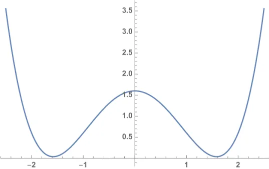
1.3 Example of potential functionV(x): α= 1, β= 3 . . . 5
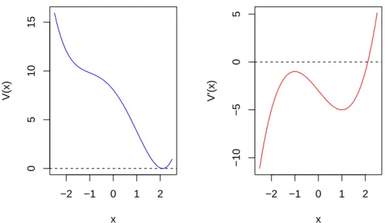
1.4 Example of potential functionV(x): α= 3, β= 3 . . . 6
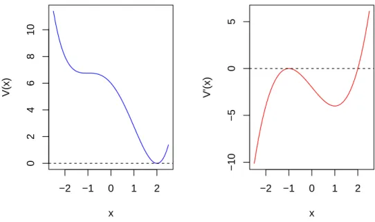
1.5 Example of potential functionV(x): α= 2, β= 3. . . 7
1.6 Cusp stationary density plots with varying asymmetry parameterα . . . 8
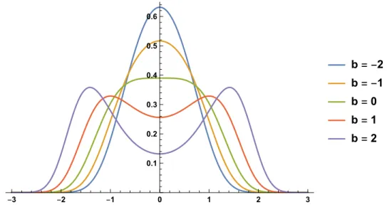
1.7 Cusp stationary density plots with varying bifurcation parameterβ . . . 8
1.8 Cusp stationary density plots with fixedβ = 3. . . 9
1.9 Example of stable and unstable market equilibria . . . 10
2.1 Sample trajectory: Cusp SDE withα= 1, β = 3. . . 24
2.2 Sample trajectory: Cusp SDE withα= 3, β = 3 . . . 25
2.3 Sample trajectory: Cusp SDE withα= 2, β = 3 . . . 26
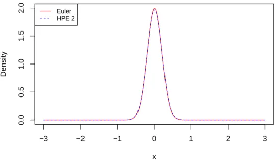
4.1 Comparison of Euler and HPE:α= 1, β = 3, x0 = 0and∆ = 0.01 . . . 46
4.2 Comparison of Euler and HPE:α= 1, β = 3, x0 = 0and∆ = 0.10 . . . 47
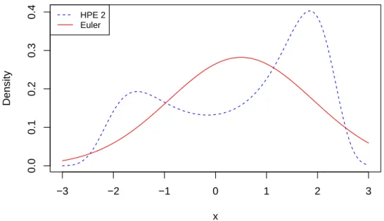
4.3 Comparison of Euler and HPE:α= 1, β = 3, x0 = 0and∆ = 0.50 . . . 47
5.1 MCMC diagnostics: Trace plot . . . 50
5.2 MCMC diagnostics: Autocorrelaiton plot. . . 51
5.3 MCMC diagnostics: Effective sample size plot . . . 52
5.4 MCMC diagnostics: Geweke plot . . . 54
5.5 MCMC diagnostics: Gelman plot forα. . . 56
5.6 MCMC diagnostics: Gelman plot forβ. . . 56
6.1 Complete observations: EmpiricalαMAPwithα= 1, β= 3. . . 60
6.3 Complete observations: EmpiricalαMAPwithα= 2, β= 3. . . 62
6.4 Complete observations: EmpiricalβMAPwithα= 2, β = 3. . . 63
6.5 Complete observations: EmpiricalαMAPwithα= 3, β= 3. . . 64
6.6 Complete observations: EmpiricalβMAPwithα= 3, β = 3. . . 65
7.1 Illustration of Bayesian data augmentation . . . 69
7.2 Partial observations: EmpiricalαMAPwith1augmented data point . . . 73
7.3 Partial observations: EmpiricalβMAPwith1augmented data point . . . 73
7.4 Partial observations: EmpiricalαMAP with2augmented data points . . . 76
7.5 Partial observations: EmpiricalβMAPwith2augmented data points . . . 76
7.6 Partial observations: EmpiricalαMAP with4augmented data points . . . 77
7.7 Partial observations: EmpiricalβMAPwith4augmented data points . . . 77
7.8 Partial observations: EmpiricalαMAP with9augmented data points . . . 78
7.9 Partial observations: EmpiricalβMAPwith9augmented data points . . . 78
7.10 Partial observations: EmpiricalαMAP with15augmented data points . . . 79
7.11 Partial observations: EmpiricalβMAPwith15augmented data points . . . 79
8.1 Bayesian hierarchical modeling: Posteriorαs . . . 82
8.2 Bayesian hierarchical modeling: Posteriorβs . . . 83
8.3 Time-varying cusp: Sample trajectories . . . 85
8.4 Time-varying cusp: Posteriorαs . . . 85
LIST OF ABBREVIATIONS AND SYMBOLS
MLE PDF SDE ϕ(z)
Maximum likelihood estimation Probability density function Stochastic differential equation
CHAPTER 1 Introduction
In modern financial econometrics, diffusion processes have been broadly applied to model the stochastic behavior of economic variables such as stock prices, interest rates, and foreign exchange rates. Well-known models such as Black-Scholes, Vasicek, and Cox-Ingersoll-Ross (CIR mdoel), all assume the underlying state variables follow diffusion processes. The thesis considers stochastic cusp model, one of the elementary catastrophe models studied in catastrophe theory.
In this chapter, we give a brief overview of cusp model including its development and appli-cations in economics. While doing so, we highlight unique characteristics which make cusp model appealing and valuable in economics and financial econometrics.
1.1 Catastrophe theory
Catastrophe theory is commonly regarded as a branch of bifurcation theory in the study of dynamic systems in mathematics. Abifurcationoccurs when a change, usually small and smooth, made to the system’s parameter values engenders a sudden “qualitative” change in its behavior. Catastrophe theory studies the mathematical characteristics of bifurcation phenomena and reveals that such bifurcations tend to occur as part of well-defined geometrical structures [Ivancevic and Ivancevic, 2007].
from attracting to repelling, and vice versa, that eventually leads to sudden “qualitative” changes of the behavior of the system [Costantino et al., 2005].
-1.0 -0.5 0.5 1.0
-2 -1 1 2
x3+x x3 x3-x
Figure 1.1:Example of degenerate singularity: functionf(x) =x3atx= 0
1.1.1 Deterministic dynamics
The dynamics of a catastrophe model is often expressed in terms of a potential functionV(x), whereV(x)is commonly approximated by polynomials. The deterministic dynamics is then gov-erned by the ordinary differential equation
dx
dt =−
dV(x;θ)
dx , x∈Randθ∈R
p. (1.1)
wherexandθdenote location and system parameters respectively. x0 is anequilibriumpoint if
dV(x)
dx |x=x0 = 0. An equilibrium pointx0 is said to be unstable if
d2V(x)
dx2 |x=x0 < 0, andx0 is a local maximum;x0 is called astableequilibrium if
d2V(x)
dx2 |x=x0 > 0,
and in this case a local minimum. An object inside the system tends to move toward the point of lowest potential. Furthermore, an equilibrium pointx0isdegenerateif d
2V(x)
dx2 |x=x0 = 0, and in this
-2 -1 1 2 0.5
1.0 1.5 2.0 2.5 3.0 3.5
Figure 1.2:Example of a quartic polynomial potential function
1.1.2 Stochastic dynamics
The stochastic version of dynamics of catastrophe model can be obtained by adding a diffusion term to Equation 1.1. The corresponding stochastic differential equation is expressed as
dXt =−
dV (Xt;θ)
dx dt+
√
εdWt. (1.2)
One common approach to gain information about Equation 1.2 is to study the transition den-sity that completely characterizes the stochastic dynamics. To better illustrate, suppose we have a diffusion processXtdescried by the SDE
dXt=µ(Xt, t;θ)dt+σ(Xt, t, θ)dWt, (1.3)
with driftµand diffusionσ.
Letp(x, t)to be the transition probability density function governed by Equation 1.3, i.e.
p(x, t)≡ d
p(x, t)is known to satisfy theFokker-Planck equation, which is also commonly known as the Kolmogorov forward equation
∂
∂tp(x, t) =− ∂
∂x[µ(x, t)p(x, t)] + 1 2
∂2 ∂x2[σ
2(x, t)p(x, t)]. (1.4)
Fokker-Planck equation describes the time evolution of the transition densityp(x, t)governed by Equation 1.3.
Unfortunately, unlike few those SDEs with simple expressions for both drift and diffusion terms, the transition densityp(x, t)of Equation 1.2 does not have analytic solution in most cases. Nonetheless, a less ambitious goal that is to obtain the stationary distribution could be achieved straightforwardly. The stationary densityπis
π(x) = N e−2Vε(x), (1.5)
whereN is the normalizing constant [Cobb, 1981] and proof is given in Appendix A.
1.2 Cusp catastrophe model
The thesis studies cusp model, one of the elementary catastrophe models developed within the framework of catastrophe theory. Cusp model considers the case when the potential is quartic polynomial, for example,
V(x;α, β) = 1 4x
4− 1 2βx
2−αx.
According to Equation 1.1, the deterministic cusp dynamics therefore has the form
dx
dt =α+βx−x
3. (1.6)
An object that obeys Equation 1.6 has equilibria when
dx
dt =α+βx−x 3
−2 −1 0 1 2
0
1
2
3
4
5
6
7
x
V(x)
−2 −1 0 1 2
−5
0
5
x
V'(x)
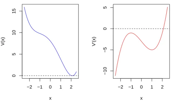
Figure 1.3:Example of potential functionV(x):α= 1, β= 3
hence finding the equilibria is equivalent to finding the roots of the cubic function
f(x) =α+βx−x3. (1.7)
Discriminant, defined as ∆disc = 27α2 −4β3 is often used as an aid to its classification of solution. In particular,
1. If∆Disc <0, Equation 1.7 will have three distinct real roots (Figure 1.3) ;
2. If∆Disc >0, Equation 1.7 will have only one real root (Figure 1.4);
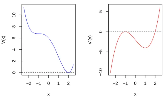
3. If ∆Disc = 0, Equation 1.7 will have two distinct roots with one of the two being a double
root (Figure 1.5).
Furthermore, the stochastic version to Equation 1.6, according to Equation 1.2 is
dXt=
(
α+βXt− 1 4X
3 t
)
dt+√εdWt, (1.8)
−2 −1 0 1 2
0
5
10
15
x
V(x)
−2 −1 0 1 2
−10
−5
0
5
x
V'(x)
Figure 1.4:Example of potential functionV(x):α= 3, β= 3
1.2.1 Cusp stationary density
According to Equation 1.5, the stationary density of the cusp stochastic differential equation has the form
π(x) = Nexp
{
2 ε
(
αx+1 2βx
2− 1 4x
4
)}
(1.9)
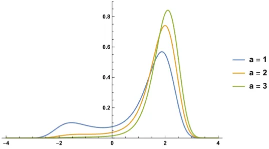
The cusp stationary density is characterized by two parametersαandβvia∆disc = 27α2−4β3. In particular,
1. If ∆disc > 0, the stationary density distribution is unimodal. The asymmetric factorα and
bifurcation factorβ measureskewnessandkurtosisrespectively (Figure 1.6).
2. If∆disc <0, the stationary density distribution isbimodal. In this caseαrepresent the relative
height of the two modes, andβ determines the separation of the two modes (Figure 1.8).
3. Moreover, the modes of stationary density (in either case) correspond to the stable equilibria of a differential equation.
−2 −1 0 1 2
0
2
4
6
8
10
x
V(x)
−2 −1 0 1 2
−10
−5
0
5
x
V'(x)
Figure 1.5:Example of potential functionV(x):α= 2, β= 3
generalization of the Gaussian, gamma, inverse gamma, and beta distributions, and belongs to the exponential family [Cobb et al., 1983]. Such flexibility makes cusp stationary density an ex-ceedingly appealing statistical model; for example it requires fewer parameters than corresponding mixture models (e.g. Gaussian mixture model) since it only needs four parameters. As pointed out by Chen et al. [2016], cusp stationary distribution is a complement to traditional approaches such as linear regression and non-parametric regression because of its capacity to simultaneously handle complex linear and nonlinear cases and the ability to capture sudden qualitative changes in dependent variables.
Cobb contributed to the development of stochastic cusp model by establishing an integrated structure for cusp stationary distribution, including parameter estimations of cusp stationary proba-bility densities using method of moments and the maximum likelihood [Cobb, 1978] [Cobb, 1981].
1.2.2 Cusp model in economics
-3 -2 -1 0 1 2 3 0.1
0.2 0.3 0.4 0.5 0.6 0.7
a=0 a=0.25 a=0.5 a=0.75 a=1
Figure 1.6: Cusp stationary density plots with varying asymmetry parameterα
-3 -2 -1 0 1 2 3
0.1 0.2 0.3 0.4 0.5 0.6
b= -2 b= -1 b=0 b=1 b=2
Figure 1.7: Cusp stationary density plots with varying bifurcation parameterβ
stationary density to US/UK rate over the period 1973 and performed model parameter estimating using MLE methods.
Fernandes [2006] provided a density matching approach for time-varying parameters with exogenous variables setting, then applied it to investigate the interest rate differential during the Swedish twin crisis empirically.
Baruník and Vosvrda [2009] fitted cusp (regression) model to US stock market data and they showed that cusp (regression) model provides a better goodness-of-fit when fitting crash of stock market data than other classic regression models such as linear regression and logistic regression.
1.3 Key research problem
Although statistical properties of cuspstationarydistribution have been well studied, unified estimating framework has established, and many empirical studies in economics or other subjects has been conducted, to best of our knowledge, little work that focuses on the actual stochastic dynamics of cusp model has been done.
One of the motivation for considering the actual stochastic cusp dynamics (Equation 1.8) comes from the application of diffusion processes in modeling stochastic behavior of economics variables in financial econometrics; it is also driven by the nature of the data one collects, in particular
time--4 -2 0 2 4
0.2 0.4 0.6 0.8
a=1 a=2 a=3
Supply
Demand
q p
Figure 1.9:Example of stable and unstable market equilibria
series data. Time series are often collected sequentially in time. If one believes that the observed time-series are generated according to some parametric specification, developing rigorous statisti-cal methods to statisti-calibrate the underlying model to measured observations has become an important research topic.
In reality, there’s always some discrepancy between continuous-time model and discrete-time observations because the underlying model is assumed to be a diffusion process hence written in continuous time, while the available observations are often sampled discretely in time, and may not becontinuousenough. This model-observation discrepancy should not be neglected, because otherwise it could lead to inconsistent estimators [Melino, 1996], [Jones, 1998], [Ait-Sahalia et al., 2008].
scenario. It is not negligible because for example, the actual transition density of the process is often approximated in some way due to intractability, a larger∆obs due to missing values would
lead to a larger deviation from the true but intractable transition density. Parameter estimation for cusp SDE with partially observed data points is a much harder case to handle.
Transition probability density
That being said, if one believes the observed values are generated according to the underly-ing parametric specification, it is naturally concerned with parameter inference for the underlyunderly-ing diffusion process Xt. Imagine data points are observed at discrete time points ti = i∆obs with
i= 0,· · · , n, and observed measurements beingx= (x0,· · · , xn).
With the assumption that the transition densityp(∆, x|x0;θ), the conditional density ofXt+∆ = xgivenXt =x0 is available in the explicit form, by Markov property, the likelihood function is
Ln(θ) = n
∏
i=1
pθ(∆, xi|xi−1)pθ(x0). (1.10)
Letℓn(θ) =logLn(θ)be the log-likelihood function, we obtain
ℓn(θ) = logLn(θ) = n
∑
i=1
logpθ(∆, xi|xi−1) +log(pθ(x0)). (1.11)
The thesis assumes pθ(X0) = 1for simplicity, since the weight of pθ(X0)in the likelihood Ln(θ)becomes negligible asnincreases.
1.4 Major contributions of the thesis
The dissertation claims following major and original contributions to the topic:
1. Under the complete observations scenario, an accurate and computationally feasible param-eter estimation algorithm based on Bayesian principle and implemented by Hamiltonian Monte Carlowas developed. Intensive simulation study was conducted and the results sup-port the claim made on the algorithm.
2. Under the partial observations scenario, three parameter estimation methods were devel-oped and compared, they are Euler approximation, closed-from approximation using Hermite polynomials by Ait-Sahalia, and Euler approximation with data augmentation. We compare the performances of three different methods by running intensive simulation studies. The result shows that the Euler approximation with data augmentation outperforms the other two in the demonstrated cases.
3. Motivated by real-world problems when only sparsely sampled observations are available (for example, longitudinal-type of data), we also investigated how the number of augmented data points would affect the parameter estimation result by simulation studies.
4. The parameter estimation algorithm was extended to more complex settings, namely the Bayesian hierarchical modeling and cusp model with time-varying parameters. The accuracy of the algorithm is supported by simulation study whose result is also presented in the thesis.
1.5 Dissertation structure
chapter 3 reviews the basics of Bayesian inference as well as Markov Chain Monte Carlo as a means to sample intractable posterior distribution. We introduce Metropolis-Hasting algorithm and Hamiltonian Monte Carlo from a practitioner’s perspective focusing on their motivation and implementation. We also highlight the ability of Hamiltonian Monte Carlo that reduces correlation between successive draws by utilizing Hamiltonian dynamics.
chapter 4 reviews two approaches to approximate the intractable cusp transition density, they are (1) closed-form approximation using finite Hermite polynomials by Sahalia [2002], Ait-Sahalia et al. [2008], and (2) the Euler approximation. We compare two different approximations by examining their plots with different time increments.
chapter 5 reviews MCMC convergence diagnostics. Regardless of whether the parameter esti-mation results are satisfying or not, it is necessary to make sure the obtained samples were indeed coming from the stationary distribution (hence the target posterior distribution) of the constructed Markov chain as we expect. Several commonly used MCMC convergence diagnostics are intro-duced and implemented to spot anything undesired.
chapter 6 contains an intensive simulation study under the complete observations scenario. The results support the claim that the proposed parameter estimation algorithm is accurate and computationally feasible.
chapter 7 considers the partial observation scenario. We introduce the idea behind formulating partial observation as missing value problem and attempt to improve the estimation accuracy with data augmentation. Simply saying, data augmentation in Bayes treats those unobserved or missing data points between two consecutive observed as unknown parameters in addition to the unknown model parameters. In particular, our simulation study shows that data augmentation outperforms both closed-form approximation by Hermite polynomials and Euler approximation in demonstrated cases. We also investigated how number of augmented data points would affect the parameter estimation result by running simulation studies.
CHAPTER 2 Numerical Methods
Cusp SDE, like most of SDEs, does not have explicit or analytic solution. Consequently, trajectory simulation is needed in order to gain information about it. By choosing and implementing appropriate discretization schemes, numerical simulations give approximations to the continuous solutions to the underlying cusp SDE. In this chapter, we review the basics of numerical methods for SDE.
2.1 Convergence criteria
Methods of approximation scheme are often classified based on the task objective. If one is interested in the whole trajectory, then it requiresstrong convergence; for other cases that one only needs approximation to some functional properties such as moment and distribution, weak convergence is often adequate.
In practice, the choice of the convergence criterion is determined by the type of the problem one is to investigate, and is often specified before constructing a numerical method and optimizing its efficiency with respect to the chosen convergence criterion [Platen, 1999].
Definition 1. A time discretizationΠN([0, T])over the time interval[0, T]contains points
0 =τ0 < τ1 <· · ·< τn <· · ·< τN =T,
2.1.1 Strong convergence
Definition 2. A time-discretized time approximation
Yn:=Yτn, n∈ {0,· · · , N}
of a continuous-time processXt, t ∈ [0, T] governed by an SDE converges in thestrong sense with orderγ ∈(0,∞]if for any fixed time horizonT it holds true that
E|YN −XT| ≤K∆γ (2.1)
for all step-sizes∆∈(0,1)andK is a constant not depending on∆.
Strong convergence criterion should be used when the task involving trajectory simulations directly. For example, simulation of a stock price usually requires the simulated sample trajectory to be close to the solution of geometric Brownian motion, and similarly simulation of a short-term rate usually requires the simulated sample trajectory be close to the solution Ornstein–Uhlenbeck process. In these cases, numerical methods are classified according to their strong orderγ of con-vergence, using the absolute error
E|YN −XT|
at the terminal timeT.
2.1.2 Weak convergence
Definition 3. A discrete time approximationY of a solutionX of an SDE converges in theweak sense with orderβ ∈(0,∞]if, for any polynomialg, there exists a constantKg <∞such that
|E(g(YN))−E(g(XT))| ≤Kg∆β (2.2)
If one is only interested in computing some functional such as probability distributions or moments that does not require us to approximate the entire trajectory of X, strong convergence criterion that requires an almost exact replica of the sample path of the solution of the underling SDE may not be necessary. One typical example is the Monte Carlo simulation of option prices at a terminal timeT, where option prices can be approximated by simply random walk instead of Brownian motion due to the fact that its first two moments (mean and variance) match the ones for Brownian motion correspondingly. In such cases, approximations of probability distribution that corresponds toX is often sufficient, and consequently only a much weaker type of convergence is needed.
Theorem 1. β ≥α(Weak order≥Strong order)
Proof. Suppose|f′| ≤K, then by mean value theorem∫ g−h≤∫ |g−h|
|Ef(YN)−Ef(XT)|≤E|f(YN)−f(XT)|
≤KE|YN −XT|
≤K(E|YN −XT|2
)1/2 .
2.2 Ito-Taylor expansion
Taylor series expansion plays an essential role in numerical analysis. For a sufficiently smooth functionf(x)in a neighborhood of some given pointx0, one could obtain approximations to any desired order of accuracy by truncating the Taylor series up to certain term.
We now briefly review the derivation of Ito-Taylor expansion, which plays the role of Taylor series in the stochastic setting.
Given a diffusion processX(t)that obeys
we make a further assumption that µ = µ[X(t)], µ = µ[X(t)](i.e. they do not depend on time explicitly).
Applying Ito lemma to any twice differentiable functionf would lead to
df[X(t)] =
{
µ ∂
∂Xf[X(t)] + 1 2σ
2
[X(t)] ∂ 2
∂X2f[X(t)]
}
dt+σ[X(t)] ∂
∂Xf[X(t)]dW(t). (2.4)
To simplify the expression, we define the following two operators:
L0 ≡µ ∂
∂X +
1 2σ
2[X] ∂ 2
∂X2 and L
1 ≡σ[X] ∂ ∂X.
Hence Equation 2.4 can be notation-wise simplified to
df[X(t)] =L0f[X(t)]dt+L1f[X(t)]dW(t). (2.5)
An equivalent expression in integral form gives
f[X(t)] = f[X(t0)] +
∫ t
t0
L0f[X(s)]ds+
∫ t
t0
L1f[X(s)]dW(s). (2.6)
Since Ito lemma holds for any twice differentialble function f, if we specify our choice of functionf(x)to bef(x) = x, Equation 2.6 gives
X(t) =X(t0) +
∫ t
t0
µ[X(s)]ds+
∫ t
t0
σ[X(s)]dW(s). (2.7)
Similarly, by choosing f(x) = µ(x), andf(x) = σ(x), and apply Ito lemma, Equation 2.6 gives
µ[X(t)] = µ[X(t0)] +
∫ t
t0
L0µ[X(s)]ds+
∫ t
t0
L1µ[X(s)]dW(s), (2.8)
and
σ[X(t)] =σ[X(t0)] +
∫ t
t0
L0σ[X(s)]ds+
∫ t
t0
Substituting Equation 2.8 and Equation 2.9 into Equation 2.7 leads to
X(t) =X(t0) +
∫ t
t0 {
µ[X(t0)] +
∫ s1
t0
L0
µ[X(s2)]ds2+
∫ s1
t0
L1
µ[X(s2)]dW(s2)
} ds1 + ∫ t t0 {
σ[X(t0)] +
∫ s1
t0
L0σ[X(s
2)]ds2+
∫ s1
t0
L1σ[X(s
2)]dW(s2)
}
dW(s1). (2.10)
Note that, in the above equation, µ[X(t0)]andσ(t0)]are inside integrand, however both re-mains constant in time. Therefore, we separate the two terms out from the remaining terms, which leads to
X(t) =X(t0) +µ[X(t0)]
∫ t
t0
ds1+σ[X(t0)]
∫ t
t0
dW(s1) +R, (2.11)
with reminder termRbeing
R≡
∫ t
t0 ∫ s1
t0
L0µ[X(s
2)]ds2ds1+
∫ t
t0 ∫ s1
t0
L1µ[X(s
2)]dW(s2)ds1 +
∫ t
t0 ∫ s1
t0
L0
σ[X(s2)]ds2dW(s1) +
∫ t
t0 ∫ s1
t0
L1
σ[X(s2)]dW(s2)dW(s1).
(2.12)
Ito-Taylor expansion with higher order terms
Higher order accuracy could be achieved If one uses substitution repeatedly to obtain constant integrands in higher order terms. To better illustrate how substitution works, we continue working on the remainder termREquation 2.12. In particular, the very last term inR, namely
∫ t
t0 ∫ s1
t0
L1
σ[X(s2)]dW(s2)dW(s1) (2.13)
is of the lowest order in∆tinR. This is a simple rule according to thebox calculus:
Applying Ito’s lemma tof(x) =L1b(x)gives
L1σ[X(s
2)] =L1σ[X(t0)] +
∫ s2
t0
L0L1σ[X(s
3)]ds3+
∫ s2
t0
L1σ[X(s
3)]dW(s3). (2.14)
Substituting Equation 2.14 to Equation 2.13 leads to
∫ t
t0 ∫ s1
t0
L1
σ[X(s2)]dW (s2)dW(s1) =
∫ t
t0 ∫ s1
t0 {
L1σ[X(t
0)] +
∫ s2
t0
L0L1σ[X(s
3)]ds3 +
∫ s2
t0
L1σ[X(s
3)]dW(s3)
}
dW(s2)dW(s1).
(2.15)
ClearlyL1σ[X(t0)]is the constant in time, hence we separate it out from the remaining terms, which in turns leads to
∫ t
t0 ∫ s1
t0
L1σ[X(t
0)]dW(s2)dW(s1). (2.16) Note that
L1σ =σσ′,
therefore Equation 2.16 becomes
∫ t
t0 ∫ s1
t0
L1
σ[X(t0)]dW (s2)dW(s1) =σ[X(t0)]σ′[X(t0)]
∫ t
t0 ∫ s1
t0
dW(s2)dW(s1).
Consequently, Equation 2.11 becomes
X(t) =X(t0) +µ[X(t0)]
∫ t
t0
ds1+σ[X(t0)]
∫ t
t0
dW (s1)
+σ[X(t0)]σ′[X(t0)]
∫ t
t0 ∫ s1
t0
dW(s2)dW(s1) + ˜R,
(2.17)
By applying Ito’ lemma again, the double Ito’s integral gives
∫ t
t0 ∫ s1
t0
dW(s2)dW(s1) = 1
2[W(t)−W(t0)] 2− 1
2(t−t0)
Consequently,
X(t) =X(t0) +µ[X(t0)]
∫ t
t0
ds1+σ[X(t0)]
∫ t
t0
dW(s1) +σ[X(t0)]σ′[X(t0)]
{
1
2[W(t)−W(t0)] 2− 1
2(t−t0)
}
+Re
(2.18)
2.3 Euler–Maruyama method
Euler–Maruyama method is a numerical method for approximating the solution of a stochastic differential equation (SDE), and not surprisingly, it’s generalizes Euler method in ordinary differ-ential equation case. Euler-Maruyama method is obtained by truncating Equation 2.18 at the first order terms (or simply look at Equation 2.11).
Let{Xt,0≤t≤T}be a solution to the stochastic differential equation
dXt=µ(Xt)dt+σ(Xt)dWt
with initial deterministic valueXτ0over a time window[0, T]. The Euler-Maruyama approximation
ofXtis a continuous stochastic processYn:=Yτn satisfying the following iterative relation
Yi+1 =Yi+µ(Yi) (ti+1−ti) +σ(Yi) (Wi+1−Wi), (2.19)
fori= 0,1,· · · , N −1withY0 =X0 andWi+1−Wi ∼ N(0,
√
∆).
x[1] = 0.5
for (i in 2:N){
x[i] = x[i-1] + (alpha + beta * x[i-1] - x[i -1]^3) * Dt + s * rnorm(1,0,sqrt(Dt)) }
Listing 2.1:Euler’s method
2.4 Milstein method
By including the second-order term in Equation 2.18, one obtains the Milstein method which has a higher accuracy of the approximation compared to Euler method.
The Milstein method is in the following form,
Yi+1 =Yi+µ(ti, Yi)(ti+1−ti) +σ(ti, Yi)(Wi+1−Wi) +1
2σ(ti, Yi)σx(ti, Yi){(Wi+1−Wt) 2−(t
i+1−ti)}.
(2.20)
The Milstein scheme has both weak and strong order of convergence ∆, which is, not sur-prisingly, superior to the Euler–Maruyama method who has the same weak order of convergence, ∆, but inferior strong order of convergence,√∆. However in our case, since the diffusion term is constant hence does not depend onXt, Milstein method is in fact equivalent to the Euler-Maruyama method.
2.5 Cusp SDE trajectory simulations
Recall in chapter one we discussed the sign of∆Discdetermines the number of roots of a cubic
2.5.1 Three roots
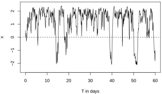
When∆Disc < 0, the cusp deterministic dynamic system has three equilibira: two stable
at-tracting equilibria divided by one repelling unstable equilibrium and the cusp stationary density distribution is bimodal.
−2 −1 0 1 2
0
1
2
3
4
5
6
7
x
V(x)
−2 −1 0 1 2
−5
0
5
x
V'(x)
Example of potential functionV(x):∆Disc<0
One sample trajectory using Euler’s method is given by Figure 2.1. In this case, we observe one appealing feature hence advantage to the stochastic cusp model over more traditionally used linear mean-reverting models in describing certain systems - that is a regime-switching type of behavior with regime being two stable equilibra. A similar behavior to this bimodal cusp SDE could be obtained by using a switching model involving two linear mean-reverting models.
2.5.2 One root
T in days
x
0 10 20 30 40 50 60
−2
−1
0
1
2
Figure 2.1: Sample trajectory: Cusp SDE withα= 1, β= 3
In this case, the cusp stationary density distribution is unimodal. According to Figure 2.2 which compares cusp model with the famous Vasicek model,
dXt =θ(µ−Xt)dt+σdWt, (2.21)
the sample trajectory exhibits stronger mean reversion than the mean-reverting models with Gaus-sian stationary densities (for example, Vasicek model in this case) due to the drift term contains a cubic term, which supports the claim by [Ait-Sahalia, 1996].
2.5.3 Two roots
When∆Disc = 0, the cusp deterministic dynamic system has two equilibrium, one being sta-ble and the other unstasta-ble. The unstasta-ble equilibrium corresponds to the dousta-ble root of the cubic function.
−2 −1 0 1 2
0
5
10
15
x
V(x)
−2 −1 0 1 2
−10
−5
0
5
x
V'(x)
Example of potential functionV(x):∆Disc>0
T in days
x
0 10 20 30 40 50 60
−2
0
2
4
Vasicek Cusp
−2 −1 0 1 2
0
2
4
6
8
10
x
V(x)
−2 −1 0 1 2
−10
−5
0
5
x
V'(x)
Example of potential functionV(x):∆Disc= 0
T in days
x
0 10 20 30 40 50 60
−2
−1
0
1
2
CHAPTER 3
Bayesian Inference using Markov Chain Monte Carlo
Model parameters of cusp SDE, namely asymmetry parameterαand bifurcation parameterβ, have well-defined geometric and statistical interpretations, and their values further determine the unique structural behaviors of cusp dynamics. This makes it particularly important that the model parameter values need to be estimated accurately and properly; therefore when doing statistical inference on model parameters, we would expect to include not only their most likely values or point estimations, but also the associated uncertainties, for example confidence interval estimations.
Bayesian inference is a method of statistical inference where Bayes’ theorem is used to update one’s prior belief on probability of unknown quantity based on observed data. The goal in carrying through Bayesian inference is to do parameter estimations for cusp model with discretely sampled data points. This chapter first reviews basis of Bayesian inference, followed by discussing MCMC as a means of sampling the intractable posterior distribution in our case.
3.1 Bayesian inference
When performing Bayesian inference for an unknown model parameter, one usually starts with some prior belief about it. As data comes in, one could compute and use the corresponding posterior distribution to draw conclusion about it. It is a conceptually straightforward application of Bayes’s theorem:
P(θ|x) = p(θ)p(x|θ)
p(x) , (3.1)
wherep(θ)andP(θ|x)are called thepriorandposterior distributionrespectively.
function such as likelihood function. Consequently, the uncertainty over the range of model pa-rameter values could be estimated naturally and directly.
3.1.1 Prior belief
Bayesian inference offers flexibility by incorporating prior belief into model inference. For example, if an expert (subjectively but reasonably) believes that some parameters might be more likely than others, that knowledge from the expert can be elicited and used as prior information in Bayesian inference. The combination of prior knowledge with likelihood of the observation will result in the posterior distribution. For other cases where little prior information is available, a flat prior, possibly improper, or other non-informative priors such as Jeffrey’s prior would be a more proper choice to reflect that (objective) belief.
3.1.2 Connections between MLE and MAP
In statistical inference, from Frequentists’ viewpoint, optimal model parameters are usually those which maximize the likelihood of the observations. Optimality is usually achieved by apply-ing various hill-climbapply-ing type of optimization methods. The optimization result is therefore point estimate of parameter value; one could also construct confidence intervals utilizing the asymptoti-cally Gaussian property of MLE.
In particular, Frequentists would seek for a vector of parameters,θ, that
θMLE =arg max
θ
p(x|θ),
or equivalently the log likelihood function
θMLE =arg max
θ
logp(x|θ). (3.2)
likelihood function:
θMAP=arg max
θ
p(θ|x) =arg max
θ
p(x|θ)p(θ) p(x) =arg max
θ
p(x|θ)p(θ),
(3.3)
or similarly the log-likelihood function
θMAP =arg max
θ
logp(x|θ)p(θ). (3.4)
When comparing MLE (Equation 3.2) and MAP (Equation 3.4), the only thing differs is the inclusion of prior p(θ) in MAP. It’s not so surprising to see MLE is equivalent to MAP if one chooses to use the flat prior, perhaps the simplest prior. To better illustrate this,
θMAP=arg max
θ
logp(x|θ)p(θ) =arg max
θ
logp(x|θ)×constant =arg max
θ
logp(x|θ) =θMLE.
(3.5)
3.1.3 Bayesian data augmentation
As discussed earlier, there’s a discrepancy between the continuous underlying model assump-tion and the discretely sampled data points in reality. The discrepancy is even more magnified when the observed data points are considerably sparse.
3.1.4 Motivation of MCMC in Bayesian inference
In Bayesian inference, once prior knowledge is incorporated into the statistical model or the likelihood function, one expects to perform Bayesian analysis based on the posterior distribution. Unfortunately, posterior distributions do not have explicit analytic forms in most cases. One way to resolve this is to utilize prior distribution that is conjugate with respect to the underlying statistical model. In this conjugate case, posterior distributionp(θ|x)is in the same probability distribution family as the prior distributionp(θ)so that one could easily obtain posterior distribution in analytic form. However this approach often fails when the specified prior is not conjugate.
Since analytic posterior distribution is difficult to obtain, a different approach would to obtain posterior distribution empirically. In particular, one would aim for taking a collection of samples that are draw from the posterior distribution, and we hope this collection of samples could be used to represent the true but intractable posterior distribution.
Vanilla Monte Carlo would not work in this case, since it still requires samples to be drawn from a target distribution (posterior distribution in this case) which as analytic form, which one does not have.
Markov Chain Monte Carlo (MCMC) provides an alternative route to the vanilla Monte Carlo. MCMC, as its name suggests, utilize a knowingly constructed Markov chain whose equilibrium distribution is the target distribution. In Bayesian inference, the target distribution is usually the posterior distribution. To better explain, let’s assume one would like to draw samples from a target distributionp(θ|x)with a prior distributionp(θ). According to Bayes’ theorem
p(θ|x) = ∫ p(θ)p(x|θ)
p(η)p(x|η)dη, (3.6)
distribu-tion
{θ(1),· · ·, θ(S)}
approximatesp(θ|x).
In this section we introduce two MCMC methods, namely the Metropolis-Hasting algorithm and Hamiltonian Monte Carlo. Since there’s really a huge literature on MCMC and HMC, we de-cide to take the practitioner’s approach focusing on their implementations rather than the theoretical justification. This chapter greatly benefits from Brooks et al. [2011].
3.2 Metropolis-Hasting
That being said, MCMC involves construction of a Markov chain whose stationary distribution is the target distribution. To better illustrate, let’s assume there already exists a collection of
sam-ples{θ(1),· · · , θ(s)}whereθ(s) being the latest draw. Now we would like to expand the existing
collection by adding some new valueθ(s+1) to it.
3.2.1 Construction of a Markov chain
Start with a proposal valueθ∗, which often close to the latest drawθ(s). The question is whether the proposed valueθ∗should be included into the existing collection or not. Intuitively, for any two different valuesθaandθb, one should expect
#{θ(s) ’s in the collection =θ a
}
#{θ(s)’s in the collection =θ b}
≈ p(θa|y)
p(θb|y)
(3.7)
in the collection [Hoff, 2009].
because
r = p(θ ∗|y) p(θ(s)|y) =
p(y|θ∗)p(θ∗) p(y)
p(y)
p(y|θ(s))p(θ(s)) =
p(y|θ∗)p(θ∗)
p(y|θ(s))p(θ(s)) (3.8) One great advantage over the vanilla Monte Carlo is that the target distribution only needs to be proportional to the posterior distribution. This means evaluation the intractable marginal likelihood is not required, which is just a normalizing constant in parameters of interest.
3.2.2 Algorithm
The Metropolis algorithm produces a valueθ(s+1) as follows:
1 Start with a collection of samples{θ(1),· · ·, θ(s)}whereθ(s)being the latest draw; 2 Generate a proposal parameter valueθ∗ according to some proposal functionJ(θ|θ(s))
-usually random-walk type;
3 Compute the acceptance ratio:
r= p(y|θ
∗)p(θ∗) p(y|θ(s))p(θ(s))
4 Acceptθ∗ with following acceptance-rejection criterion:
θ(s+1) =
{
θ∗ with probability min(r,1) θ(s) with probability1−min(r,1) Algorithm 1:Metropolis- Hasting algorithm
After some burn-in time, the Markov chain with accepted draws is expected to converge to the equilibrium distribution, regardless where the chain started initially. Samples after the burn-in time would be a good empirical approximation to the true target distribution. More detailed assessment on convergence of the chain is given in chapter 5.
3.3 Hamiltonian Monte Carlo
conver-gence to the target equilibrium distributionπ(x)slow. To reduce the correlation between successive sampled states, Hamiltonian Monte Carlo has been developed under the framework of MCMC and it differs from the Metropolis–Hastings algorithm by adopting a Hamiltonian dynamics between states to achieve the goal of reducing autocorrelation. By utilizing the gradient information rather than just the probability distribution alone, Hamiltonian Monte Carlo is able to explore the target distribution much more efficiently compared with metropolis-Hasting, resulting in faster conver-gence [Neal et al., 2011]. This section on Hamiltonian Monte Carlo benefited greatly from Neal et al. [2011]and Betancourt [2017].
3.3.1 Hamiltonian dynamics
For an object inside a dynamic system, the object’s state or motion is governed by both location x ∈ Rn and momentump ∈ Rn. There is an associated potential energy, commonly denoted by U(x)for each location the object takes; and similarly there’s an associated kinetic energy commonly denoted by K(p) for each momentum the object posses. We say the object obeys Hamiltonian dynamics if the total energy is conserved; in this case, the total energy is called the Hamiltonian, denoted byH(x, p), which is defined as the sum of potential and kinetic energies for a given object:
H(x, p) =U(x) +K(p) (3.9)
Hamiltonian dynamics expresses how kinetic energy and potential energy are converted to one or the other as an object inside a system moves in time, and it is mathamatically described by the Hamiltonian equations:
∂xi
∂t =
∂H ∂pi ∂pi
∂t =−
∂H ∂xi
(3.10)
for given expressions for ∂H∂x
i and
Once Equation 3.10 as well as an initial positionx0 and initial momentump0 at time t0 are given, both the location and momentum of an object at some future timet=t0+∆can be computed by simulating these dynamics for∆unit of times.
3.3.2 The Leap Frog Method
The Hamiltonian equations (3.10) describe an object’s motion in time, and the trajectory is continuous in time. It is necessary to approximate the Hamiltonian equations by discretizing over time, in order to numerically simulate the trajectory. This can be usually achieved by theLeap Frog method:
1. Take a half step forward in timeδ/2to update the momentum variable while fixing position variable att:
pi(t+δ/2) =pi(t)−(δ/2) ∂U ∂xi
(t);
2. Take a full step forward in time to update the position variable while fixing momentum vari-able computed at timet+δ/2from previous step:
xi(t+δ) = xi(t) +δ∂K ∂pi
(t+δ/2);
3. Take the remaining half step in time to finish updating the momentum variable while fixing position variable at timet+δ:
pi(t+δ) = pi(t+δ/2)−(δ/2) ∂U ∂xi
(t+δ).
3.3.3 The target distribution
By developing a Hamiltonian functionH(x, p), the resulting Hamiltonian dynamics could be used to efficiently explore the target distributionπ(x).
For any energy functionE(θ)over a set of variablesθ, the corresponding Gibbs’ canonical distributioncan be defined as:
π(θ) = 1 Ze
−E(θ)
(3.11)
whereZis the normalizing constant. The Hamiltonian is the sum of potential and kinetic energies:
E(θ) =H(x, p) =U(x) +K(p) (3.12)
The canonical distribution for the Hamiltonian dynamics energy function is defined as
π(x, p)∝e−H(x,p)=e−[U(x)−K(p)] =e−U(x)e−K(p)∝π(x)π(p) (3.13)
The fact that the joint distribution forxandpfactorizes implies that the canonical distribution π(x) is independent of the analogous distribution for the momentum π(p). By introducing mo-mentum asauxiliary variables, the Markov chain path could be facilitated based on Hamiltonian dynamics; it would not be possible without momentum. Due to the independence of the canonical distributions forxandp, theoretically any distribution for sampling momentum variables could be used. A zero-mean Normal distribution with unit variance is a often good choice for the momentum variables.
K(p)∝ p Tp
2 (3.14)
3.3.4 Algorithm
By achieving so, HMC consists of the two alternating steps: one is a stochastic step that per-forms random transition between energy levels, the other is a deterministic step that perper-forms leapfrog method along a given energy level followed by determining whether or not accept the proposal based on the Metropolis acceptance-rejection criterion.
Let(xt−1, pt−1)be the latest draw in the chain. To illustrate how the two alternative steps work, let’s suppose we are at an initial state(x0, p0) = (xt−1, pt−1), numerical simulation using the Leap Frog methods is performed according to Hamiltonian dynamics for a short time, which leads to a new state denoted by(x∗, p∗)at the end of the simulation, and further used as theproposal. Due to inevitable discretization error, Metropolis acceptance criterion is used again here to determine whether or not the proposed state is accepted. Specifically if the probability of the proposed state after Hamiltonian dynamics
π(x∗, p∗)∝e−[U(x∗)+K(p∗)] (3.15)
is greater than probability of the state prior to the Hamiltonian dynamics
π(x0, p0)∝e−[U(x
(t−1)),K(p(t−1))]
(3.16)
then the proposed state is accepted; otherwise, the proposed state is accepted randomly with a computed ratio.
all ofπ(x), which can be achieved by simply drawing a random momentum from the corresponding canonical distributionπ(p)before running the dynamics prior to each sampling iteration.
1 Start with a collection of samples{x(1),· · · , x(s)}wherex(s)being the latest draw; 2 Letx0 bex(s);
3 Sample a new initial momentum variablep0frompi(p);
4 RunLeap Frog algorithmstarting at[x0, p0]forLsteps with step-sizeδto obtain proposed statesx∗andp∗ ;
5 Compute the acceptance ratio:
r=exp(−U(x∗) +U(x0)−K(p∗) +K(p0))
6 Acceptθ∗ := (α∗, β∗)with following acceptance-rejection criterion:
θ(s+1) =
θ∗ with probability min(r,1) θ(s) with probability1−min(r,1)
CHAPTER 4
Transition Density Approximations
In previous chapter, we reviewed MCMC as a means to sample intractable posterior distribu-tion in Bayesian inference, and we also showed posterior distribudistribu-tion requires an explicit likelihood function. However the transition density of cusp dynamics, hence the likelihood function is ana-lytically intractable, approximation to the transition density is therefore needed. In this chapter, we review two different approaches to approximate the transition density of cusp SDE.
4.1 Motivation
Consider a diffusion processXtgoverned by
dXt =µ(Xt;θ)dt+σ(Xt;θ)dWt, (4.1)
whereµandσare known functions that both might depend on a vector of model parametersθ. Let pX(∆, x|x0;θ)be the conditional density of Xt+∆ = x given Xt = x0 induced by the model Equation 4.4, the transition probability density. Further assume data points are observed at discrete time points ti = i∆obs with i = 0,· · · , n, and observed measurements being x =
(x0,· · · , xn). Due to Markovian property, the log-likelihood function has the simple form
ℓn(θ)≡ n
∑
i=1
ln{pX
(
∆, Xi∆|X(i−1)∆;θ
)}
4.2 Closed-form approximation using Hermite polynomials
Ait-Sahalia [2002] develops two approaches to construct a sequence of closed-form expansions for the log-likelihood function that approximate the intractable (log) transition density of a diffusion process. One is based on finding the coefficients of a Hermite expansion for the transition density; the other takes the form of the Hermite series first, and computes its coefficients by solving the Fokker-Planck equation which characterize the transition function. The two approaches give the same final expression [Ait-Sahalia et al., 2008].
4.2.1 Hermite polynomials
The modified Hermite polynomial with degreenis denoted by
Hn(z) = ez2/2 d n
dzn
(
e−z2/2
)
, n ≥0. (4.3)
If we letϕ(z)be the pdf of the standard normal distribution,Hnhas the property
∫ ∞
−∞
ϕ(z)Hn(z)Hm(z)dz =
0 n̸=m
n! n=m
4.2.2 Derivation
Consider a continuous-time parametric diffusion
dXt =µ(Xt;θ)dt+σ(Xt;θ)dWt, (4.4)
First transformation
First, applying the Lamperti transformationγ(·)toXtgives us a transformed new processYt such that
Yt =
∫ Xt du
σ(u;θ). (4.5)
By Ito’s lemma, the transformed processYtsatisfies the following SDE
dYt=µb(Yt;θ)dt+dWt, (4.6)
with drift term being
b
µ(Yt;θ) =
µ(X;θ) σ(Xt;θ)
− 1
2
∂σ(Xt;θ)
∂x ,
and unit diffusion term.
Second transformation
LetYtbe the value ofY corresponding toXt, and we further transformYtby normalizing it in
Z = Y√−Yt
∆ . (4.7)
Intuitively, the transition density ofp(Zt+∆|Zt = zt)is well, or at least better approximated by Gaussian with meanµb(Yk;θ)
√
∆and unit variance. Hence, it suggests using Hermite series expansion to approximate the transition densityf(z, t)
f(z, t) = ϕ(z) ∞
∑
n=0
ηn(z, t)Hn(z), (4.8)
Hermite series expansion
To approximate the transition density, Ait-Sahali proposed to take the form of the Hermite series and determines its coefficients by solving the Fokker-Planck equation which characterize the transition function. In particular, first rewrite Equation 4.8 as
f(y, t) = √1 2πtexp
(
−(y−Yk)2
2t
)
×ψ(y, t)exp
(∫ y
Yk b
µ(u)du
)
. (4.9)
The right hand side of equation Equation 4.9 is the product of ϕ(z)expressed in terms of Y and two remaining terms that plays the role of the infinite Hermite sum in Equation 4.8.
The goal is to expressψ(y, t)in terms of a convergent power series int, where the coefficients of the series are expected to capture the contribution made by the entire family of Hermite poly-nomials at each order int. In particular a desiredψ is in the form of a power series expansion in t,
ψ(y, t) = ∞
∑
n=0
cn(y)tn
n! , (4.10)
and coefficients are to be determined.
To achieve so, the unit diffusion process Yt is known to satisfy the Fokker-Planck equation, which gives
∂f
∂t =−µb ∂f ∂y −f
∂µb
∂y +
1 2
∂2f
∂y2. (4.11)
Solution of equation Equation 4.11 may be represented by expression Equation 4.9 provided ψ(y, t)satisfies
∂ψ
∂t =
1 2
∂2ψ ∂y2 −
y−Yk t
∂ψ
∂y +λψ, λ=−
1 2
( b
µ2+∂bµ ∂y
)