Research Article Goal-Programming-Driven Genetic Algorithm Model for Wireless Access Point Deployment Optimization

(1)

Volume 2012, Article ID 780637,14pages doi:10.1155/2012/780637

Research Article

Goal-Programming-Driven Genetic

Algorithm Model for Wireless Access Point

Deployment Optimization

Chen-Shu Wang

1

_{and Ching-Ter Chang}

2

1_{Graduate Institute of Information and Logistics Management, National Taipei University of Technology,}

Taipei 10608, Taiwan

2_{Department of Information Management, Chang Gung University, Tao Yuan 333, Taiwan}

Correspondence should be addressed to Chen-Shu Wang,[email protected]

Received 24 February 2012; Accepted 8 May 2012 Academic Editor: Jung-Fa Tsai

Copyrightq2012 C.-S. Wang and C.-T. Chang. This is an open access article distributed under

the Creative Commons Attribution License, which permits unrestricted use, distribution, and reproduction in any medium, provided the original work is properly cited.

Appropriate wireless access point deploymentAPD is essential for ensuring seamless user

communication. Optimal APD enables good telecommunication quality, balanced capacity loading, and optimal deployment costs. APD is a typical NP-complex problem because improving

wireless networking infrastructure has multiple objectivesMOs. This paper proposes a method

that integrates a goal-programming-driven modelPMand a genetic algorithmGAto resolve

the MO-APD problem. The PM identifies the target deployment subject of four constraints: budget, coverage, capacity, and interference. The PM also calculates dynamic capacity requirements to replicate real wireless communication. Three experiments validate the feasibility of the PM. The results demonstrate the utility and stability of the proposed method. Decision makers can easily refer to the PM-identified target deployment before allocating APs.

1. Introduction

Appropriate wireless access point deploymentAPDis essential for ensuring seamless user communication. Optimal APD enables good telecommunication quality, balanced capacity loading, and optimal deployment costs. APD is a typical NP-complex problem1because it involves multiple decision objectives, such as budget2–4, coverage2,5–8, interference

3,4,7, and dynamic capacity1,4,6–9. Furthermore, these objectives usually contradict each other7. For example, the number of APs is usually positively related to the wireless signal coverage rate and telecommunication reliability 1. However, more APs increase deployment costs. These conflicting criteria should be considered simultaneously when solving APD problems9,10.

(2)

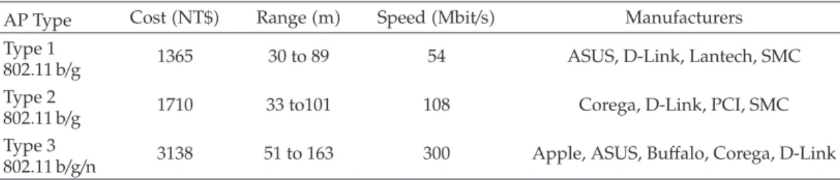
Table 1: A comparison of the three wireless AP types.

AP Type CostNT$ Rangem SpeedMbit/s Manufacturers

Type 1

802.11 b/g 1365 30 to 89 54 ASUS, D-Link, Lantech, SMC

Type 2

802.11 b/g 1710 33 to101 108 Corega, D-Link, PCI, SMC

Type 3

802.11 b/g/n 3138 51 to 163 300 Apple, ASUS, Buﬀalo, Corega, D-Link

In the last decade, many studies have attempted to solve APD optimally by considering multiple objectives MOs. There are four main objectives: budget, coverage rate, capacity, and interference. Studies have attempted to identify maximal coverage. For example, Huang et al. developed a growth-planning algorithm to establish the maximal coverage range11. Zhao et al. used a point-to-point signal strength strategy to implement indoor AP location optimization for maximal coverage12. For the capacity objective, the capacity requirements of wireless networks compared to wired networks are particularly diﬃcult to evaluate because users are dynamic and can move from place to place. This makes APD a dynamic and complex problem. The dynamic capacity requirement must be addressed to resolve APD 13 because users can access particular APs to balance loads 9, 14. Finally, for the interference objective, too many APs of the same type and placed too close together may cause AP malfunction because of frequency interference. To avoid communication interference, some studies 6, 15 have suggested that APs should be arranged on diﬀerent communication channels, but this leads to other communication channel assignment problems.

This paper applies a goal-programming-driven modelPMto the MO-APD problem. It uses goal programmingGPto infer and model the PM and a genetic algorithmGAto search for near optimal solutions. These methods are easily applied to MO-APD problems to reflect real situations. The remainder of this paper is organized as follows:Section 2defines the problem; Section 3details the PM;Section 4 presents a discussion on the PM solution process using a GA;Section 5provides the results of numerical experiments which are given in this section; lastly,Section 6oﬀers a conclusion and suggestions for future research.

2. Description of the APD Problem

This research resolves the MO-APD problem according to four decision constraints: budget, coverage, capacity requirements, and interference. The PM identifies a feasible target deploymentT, which consists of three types of wireless APs, as shown inTable 1. This study conducted experiments and surveys that indicate that the coverage range and communication speed of a Type 3 AP are wider and faster, respectively, than AP Types 1 and 2. However, Type 1 AP equipment is cheaper than AP Types 2 and 3. Two APs may interfere with each other if they are the same type and are too near. Therefore, the PM must balance the four decision con-straints and allocate three AP types in the target deployment of the APD problem.Table 2lists the variables used in the proposed models.

(3)

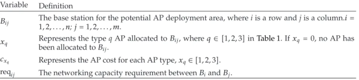
Table 2: Variables used in this paper.

Variable Definition

Bij The base station for the potential AP deployment area, where i is a row and j is a column.i

1,2, . . . , n;j1,2, . . . , m.

xq Represents the type q AP allocated toBij, whereq∈1,2,3inTable 1. Ifxq0, no AP has

been allocated toBij.

cxq Represents the AP cost for each AP type,xq∈1,2,3.

req_ij The networking capacity requirement betweenBiandBj.

2.1. The Budget Constraint

θT

Budget is the most important APD-MO constraint that directly aﬀects the feasibility ofT. The cost function in2.1evaluates the total cost ofT. Equation2.2evaluates the budget constraint. In2.2, bgt represents the given budget constraint for the AP allocation forT:

CSTT

i

j

CxqBi,j, ∀Xq/0, i1,2, . . . , n, j 1,2, . . . , m, _2.1

if CSTT<bgt, θT 1, elseθT bgt

CSTT.

2.2

2.2. The Coverage Constraint

ΦT

Figure 1 shows that to enable seamless user communication, two APs are allocated, but two capacity requirementsreq_2,1and req_2,3have no signal coverage. The coverage function

CVGT evaluates the signal coverage area ofT. Equation 2.3 evaluates the coverage fulfillment rate:

ΦT CVGT

target area. 2.3

2.3. The Capacity Constraint

ΨT

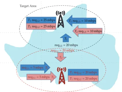
Figure 2shows a dynamic capacity scenario. The target area allocates two Type 1 APsAP1

and AP2, and two APs simultaneously cover the capacity requirementsreq22. For time

slot 1T1, the capacity requirements of req₁₂,req₁₃,and req₂₂ access AP1, and the capacity

requirements of req₃₁ and req₃₂ access AP2. Therefore, for time slotT1, AP1 and AP2 must

provide 55 and 25 mbit/s capacity, respectively. In time slotT2, req₂₂ shifts connection from

AP1 to AP2 for balance loading. Therefore, for time slot T2, AP1 and AP2 must provide 35

(4)

req req req

req

req req

Target Area

1,1 1,2

1, m

2,1 2,2 2, m

n,1

n,2 3,3

Figure 1: The signal coverage illustration.

Target Area

T1

T1 req1,2=25 mbps T1

T1 req1,2=25 mbps

T1req1,3=10 mbps T2

T2

req1,3=10 mbps

req3,1=5 mbps

T1req3,2=20 mbps

req2,2=20 mbps

Figure 2: The dynamic capacity requirements of two APs. The blue area represents time slot 1T1and the

pink area represents time slot 2T2.

A Monte Carlo simulation algorithm—that simulates the capacity of T—implements the DCP_ijTfunction. Equation2.4evaluates the capacity fulfillment rate:

if DCPijT>req_ij, ΨT 1, i1,2, . . . , n; j1,2, . . . , m,

elseΨT DCPijT req_ij .

(5)

Target Area

B2,2

B1,1 B₁_,₂ B1,m

B2,1 B2,m

Bn,1

Bn,2

B3,3 Type 1 AP

Type 1 AP

Type 2 AP

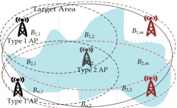
Figure 3: The frequency interference illustration.

2.4. The Interference Constraint

ωT

Figure 3 shows that many Type 1 APs are used to maximize coverage and capacity of T because of budget constraints. However, too many APs of the same type and allocated too near to each other may lead to AP malfunction because of AP frequency interference. For example, Figure 3 shows a perfect coverage design. However, it also shows an increased interference rate. The interference function IFTT evaluates the interference area of T.

Equation2.5evaluates the interference fulfillment rate:

ωT 1− IFTT

target area. 2.5

3. Proposed Model to Solve MO-APD

Two main approaches can be used to formulate MO-APD. One approach is the cost-oriented approach, which aims to minimize total cost subject to MO performance constraints. This study formulated MO-APD using the cost-oriented approach as shown in Proposal 1 P1. GAL-CVG, GAL-CP, and GAL-IFT are the given constraints for coverage rate, capacity fulfillment rate, and interference fulfillment rate, respectively.

P1

Min CSTT≤bgt, 3.1

subject to

ΦT≥GAL−CVG, 3.2

ΨT≥GAL−CP, 3.3

(6)

Equations3.2–3.4are the coverage, capacity, and interference constraints. Equation

3.1is the objective function, which minimizes the total cost subject to multiple decision constraints3.2–3.4.

The second approach is performance oriented, and it maximizes the performance of target deployment subjects to real constraintse.g., budget. This study reformulated the MO-APD using the performance-oriented method, shown in Proposal 2P2.

P2

MaxΦT ΨT ωT, 3.5

subject to3.1–3.4.

Equation3.5is the objective function in P2, which maximizes the coverage, capacity fulfillment, and interference fulfillment rates of T subject to budgetary 3.1 and other decision constraints 3.2–3.4. GP aids MO decision-making problem modeling. It was first introduced by Charnes and Cooper 16and further developed by Tamiz et al. 17, Romero18, and Chang19. Various types of GP approaches exist, such as lexicographic GP, weighted GP, MINMAXChebyshevGP, and multichoice GP19. To enable decision makers to easily set the constraint weighting according to their preferences, this study used a weighted GP approach to translateP2into the PM.wcvg,wcp, and wIFTare the

important weightsbetween 0 and 1for the GAL-CVG, GAL-CP, and GAL-IFT constraints, respectively.

PM

Min Wbgt

bgtWcvg

cvg−Wcp

cp−WIFT

IFT−, 3.6

subject to

CSTT−bgtbgt−bgt, 3.7

ΦT−cvgcvg−GAL−CVG, 3.8

ΨT−cpcp−GAL−CP, 3.9

ωT−IFTIFT−GAL−IFT, 3.10 bgt,bgt−,cvg,cvg−,cp,cp−,IFT,IFT−≥0. 3.11

4. Process for Solving the PM Using a GA

The GA is a stochastic searching method that uses the mechanics of natural selection to solve optimization problems. The GA was developed from the theory of natural selection

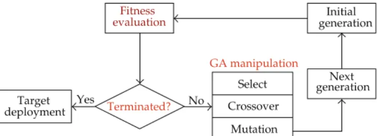
20. Because the GA is a good stochastic technique for solving combinatorial optimization problems, this study uses the GA as the PM search tool, as shown inFigure 4.

An initial solution population is randomly created. The fitness of each individual in the population then determines whether it survives. Termination criteriasuch as the generation size or the fitness value exceeding the thresholddetermine the target deploymentTto be achieved. Finally, genetic operators such as selection, crossover, and mutation identify the

(7)

Initial generation

Terminated?

Select Crossover

Mutation

GA manipulation

Target deployment

No Yes

Fitness evaluation

Next generation

Figure 4: GA-based PM solution process.

next generation. After meeting a number of iterations or predefined criteria, a near optimal solution is found.

4.1. Representation Structure: Encode/Decode

A graph represents a target deploymentTthat can also be expressed as a two-dimensional matrix. In the graph, each potential base stationBi,jhas two states: APBi,j 1allocated

and no APBi,j 0allocated. A base station with an allocated AP must have an AP type

xq 1,2,3.n×mbit strings were used as chromosomes to representT :

T

⎡ ⎢ ⎢ ⎢ ⎣

B1,1 B1,2 · · · B1,m

B2,1 B2,2 · · · B2,m

..

. ... ... ...

Bn,1 Bn,2 · · · Bn,m

⎤ ⎥ ⎥ ⎥

⎦. 4.1

4.2. Evaluation Function

The PM objective functionFiwas used as a GA evaluation function in4.2. All variables in4.2are defined as in the PM:

Fi Wbgt

bgtWcvg

cvg−Wcp

cp−WIFT

IFT−. 4.2

4.3. GA Manipulations

1Selection: roulette wheel selection ensures that highly fit chromosomes produce

more oﬀspring. This method selects a candidate network according to its survival probability, which is equal to its fitness relative to the whole population, as shown in4.3:

_F_i

_F

i

. 4.3

2Crossover: the crossover method randomly selects two chromosomes from the

(8)

4 8 3 10 5 7 10 6 8 10

7 9 5 1 3 1 6 2 2 9

0 2 5 6 5 6 4 5 3 8

6 1 8 7 5 4 9 6 2 6

0 4 7 7 8 8 10 8 3 3

10 6 8 1 4 4 6 8 9 5

4 1 9 2 8 0 8 2 7 4

3 9 2 5 8 7 1 4 8 9

8 2 7 4 4 5 8 8 10 7

6 1 9 0 6 1 5 4 6 6

Figure 5: Capacity requirements for Experiment 1.

1, n×m. Two new chromosomes, called oﬀspring, are then obtained by swapping all characters between positionCandn×m.

3Mutation: the combined reproduction and crossover methods occasionally lose

potentially useful chromosome information. Mutation is introduced to overcome this. It is implemented by randomly complementing a bit0 to 1 and vice versa. This ensures that good chromosomes are not permanently lost.

5. Experiment Validation and Analysis

To validate the efficiency and feasibility of the PM at resolving APD problems, three experiments were designed and implemented. Experiment 1 included four subtests to validate parameter combination types consisting of different decision variables. Experiment 2 included two subtests to confirm the ability of the PM to solve dynamic capacity problems. Experiment 3 ensured that the PM is suitable for large-scale problems and tested the GA parameter effects.

5.1. Experiment 1: Decision Variable Combination Validation

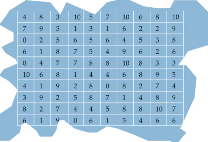
Four subtests consisting of diﬀerent decision variables and important weights validated the ability of the PM to solve APD problems. The target area inFigure 5is a 90 km2 _irregularly

shaped area. The capacity requirements inFigure 5were identical for all subtests. All req_ij could move around the target area, where signal coverage was present. For comparative purposes, the GA parameters of the four subtests—population size600, terminated gen-eration500, crossover rate0.4, and mutation rate0.1—were fixed.Table 3lists the other decision variables.

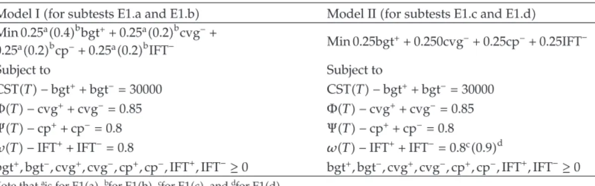
Table 4shows the four subtests formulated as Model I and Model II according to the PM. To avoid the randomizing eﬀect of the GA, all subtests were run three times with the same parameters on the same machine. The result averages are reported.Table 5shows the analysis of the experiment results. The E1.a and E1.b results show that the important budget weight is less in E1.b than in E1.a. Therefore, only 15 APson averageare deployed for E1.b,

(9)

Table 3: Decision variables and import weights for four subtests in Experiment 1.

Decision variable E1.a E1.b E1.c E1.d

Budget 30000Wbgt.25 30000Wbgt.40 35000Wbgt.25

Coverage rate 85%Wcvg.25 85%Wcvg.20 85%Wcvg.25

Capacity fulfillment rate 80%Wcp.25 80%Wcp.20 80%Wcp.25

Interference fulfillment rate 80%WIFT25 80%WIFT.20 80%WIFT25 90%WIFT25

Note that important weights are marked in parentheses.

Table 4: Model I and Model II for resolving the four subtests.

Model Ifor subtests E1.a and E1.b Model IIfor subtests E1.c and E1.d

Min 0.25a₀_.₄b_bgt₀_.₂₅a₀_.₂b_cvg₋

0.25a₀_.₂b_cp₋₀_.₂₅a₀_.₂b_IFT− Min 0.25bgt0.250cvg−0.25cp−0.25IFT−

Subject to Subject to

CSTT−bgtbgt−30000 CSTT−bgtbgt−30000

ΦT−cvgcvg−0.85 ΦT−cvgcvg−0.85

ΨT−cpcp−0.8 ΨT−cpcp−0.8

ωT−IFTIFT−0.8 ωT−IFTIFT−0.8c₀_.₉d

bgt,bgt−,cvg,cvg−,cp,cp−,IFT,IFT−≥0 bgt,bgt−,cvg,cvg−,cp,cp−,IFT,IFT−≥0

Note thata_{is for E1}_a_,b_{for E1}_b_,c_{for E1}_c_{, and}d_{for E1}_d_.

Table 5: Analysis of the results of Experiment 1.

Indicator E1.a E1.b E1.c E1.d

Fitness .9534 .9420 .9568 .9567

Times 160.0993 160.106 159.0593 170.4233

Cost 36954 29360 34647 34694

Coverage rate .85 .6967 .8167 .8233

Capacity fulfillment rate .8490 .6981 .8189 .8269

Interference fulfillment rate .94 .9867 .94 .99

Number of APs 22 15 21 23

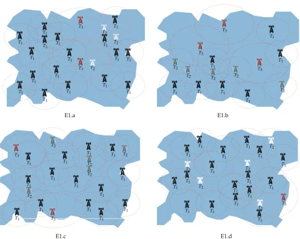
as shown inFigure 6. The results also show that the decision maker must either increase the budget or adjust the other decision objectives. For example, E1.b shows that the coverage and capacity fulfillment rates can only reach 0.7 at the current budget. As the budget increases from 30000in E1.bto 35000in E1.c and E1.d, the number of APs deployed increases to 22on average. The coverage and capacity rates increase from 0.7 in E1.b to 0.82 in E1.c and E1.d. E1.d deployed more APs23at a lower cost than E1.a22 APs.Figure 6shows that the APs in E1.c and E1.d are spread evenly in the target area to avoid interference.Figure 7 shows the convergence trends for all subtests.T emerges after 100–150 iterations.

5.2. Experiment 2: Dynamic Capacity Requirement Validation

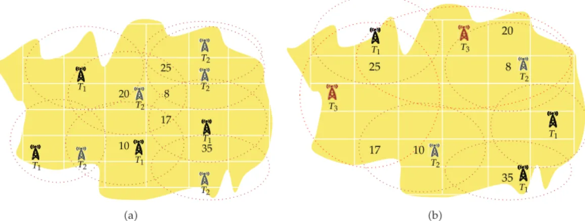
Experiment 2 consisted of two subtests to validate the ability of the PM to resolve dynamic capacity requirements.Figure 6ashows that in subtest E2.a, most capacity requirements are in the central area of the target32 km2_._{Figure 6}_b_{shows that in subtest E2.b, the capacity}

(10)

T1

T1 T1

T1

T1 T1

T1 T1 T1 T1 T1 T1

T1 T2

T2 T2 T3 T3 T T T T T T T T1 T1 T1 T1 T1 T1 T1 T2 T2 T2 T2

T2 T3

T3 T3 T1 T1 T1 T1 T1 T1 T1 T1 T1 T1 T1 T1 T1 T1 T2 T2 T2 T2 T2 T3 T3 T1 T1 T1 T1 T1 T1 T1 T1 T1 T1 T1

T1 T1

T1 T1 T1 T1 T2 T2 T2 T2 T2 T3 E1.a E1.b E1.c E1.d

Figure 6: AP deployment results for the four subtests in Experiment 1.

Table 6: Decision variable and important weights for Experiment 2.

Decision variable Variable value

Budget 15000Wbgt.3

Coverage rate 85%Wcvg.15

Interference fulfill rate 85%WIFT.15

Capacity fulfill rate 95%Wcp.4

Note that the important weights are marked in parentheses.

requirements are scattered in the corners of the target area.Table 6shows that the capacity requirements and all default decision variables are identical for both tests. The GA param-eters—population size600, terminated generation500, crossover rate0.4, and mutation rate0.1—were fixed to enable result comparison. To avoid random GA eﬀects, all subtests were run three times with the same parameters on the same machine. The result averages are reported.

Table 7shows the experiment results analysis. As expected, APD follows the capacity requirements, as shown in Figures8aand8b. Figures8aand8balso show that APs are more central in E2.a than in E2.b to fulfill the capacity requirements. Although the capacity requirements are the same in both experiments, E2.a requires nine APs, which is more than

(11)

0 100 200 300 400 500 0.84

0.86 0.88 0.9 0.92 0.94 0.96

Generations

Fitness value

E1.a E1.b

E1.c E1.d

Figure 7: The convergence trends for the four subtests in Experiment 1.

25

20 8

17

10 ₃₅T1

T1

T2

T2 a

20

25 8

17 10

35

T1

T2

T3

b

Figure 8: The capacity requirement and results of Experiment 2 forasubtest E2.a andbsubtest E2.b. The numbers represent the capacity requirements.

E2.bseven APs. Therefore, capacity requirements are dynamic, andTrequires more APs to manage the capacity requirement increase in E2.a.

5.3. Experiment 3: The Effect of Large-Scale Problems and

GA Parameters on Validation

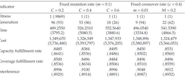
Two subtests of Experiment 3 were designed as large-scale problems.Table 8lists the decision variables and the important weights. Experiment 3 also tested GA parameter combinations, including crossover and mutation rates.

The results analysis in Table 9 shows that the PM is more sensitive to crossover rate. Generation—as an evaluation indicator for subtests E3.a and E3.b—shows that feasible deployment can be reached in the following order of crossover rates: 0.6converged by 22 iterations, 0.4converged by 70 iterations, and 0.2converged by 95 iterations. However, no such pattern exists for mutation rate in either test. Therefore, a crossover rate of 0.4 and

(12)

Indicator E2.a E2.b

Fitness 1 1

Times 5.1883 4.7797

Cost 14387 14068

Coverage rate .8518 .8518

Capacity fulfillment rate 1 1

Interference fulfillment rate .9815 .9259

Number of APs 9 APs 7 APs

Table 8: Decision variables and important weights for Experiment 3.

Objective E3.a E3.b

Target area 2250 km2 _{90000 km}2

BudgetWbgt.55 1350 000 5650000

Coverage rateWcvg.15 85% 85%

Capacity and interference fulfillment ratesWcpWIFT0.15 80% 80%

Note that the capacity requirements are shown in the Appendix and the important weights are marked in parentheses.

Indicator Fixed mutation ratem0.1 Fixed crossover ratec0.4

C0.2 C0.4 C0.6 m0.01 M0.2

Fitness 1.9869 11 11 11 11

Generation 9693 5386 1826 994 2262

Time 489.2550 3795.2 526.2310 5080.5 552.5640 3880.6 496.0540 3334.8 541.5390 4866.5 Cost 1,349,670 5,736,480 1,326,549 5,593,797 1,347,933 5,576,205 1,348,896 5,580,897 1,324,479 5,566,053

Capacity fulfillment rate .8485

.8641 .8384 .8536 .8495 .8486 .8450 .8502 .8531 .8560

Coverage fulfillment rate .8500

.8536 .8496 .8634 .8484 .8506 .8496 .8510 .8496 .8559 Interference .8996

.8929 .9100.8914 .8891.8996 .9048.8987 .9012.8952

The experiment results for E3bare in parentheses.

a mutation rate of 0.1 are recommended for experiment implementation to avoid GA parameter eﬀects. The results inTable 9show that large-scale problemsE3.bcan be resolved within an acceptable time4191.52 s, approximately 1 h.

6. Conclusion

Optimal wireless LANWLANdesign is important to ensure seamless user communication. Appropriately locating wireless APs for WLANs is important. Optimal APD enables high telecommunication quality, balanced capacity loading, and optimal deployment costs. This study proposes a GP-driven model integrated with a GA to solve MO-APD subject to four constraints: budget, capacity, interference, and coverage. The experiment results show that

(13)

Figure 9: Capacity requirements for Experiment 3.a.

the PM resolves many APD problems and achieves dynamic capacity replication. Results confirm the ability of the PM to solve large-scale APD problems. Future research should focus on other applications and further verification of PM.

Appendix

Figure 9shows the capacity requirement for the E3.a subtest.

References

1 N. Weicker, G. Szabo, K. Weicker, and P. Widmayer, “Evolutionary multiobjective optimization for

base station transmitter placement with frequency assignment,” IEEE Transactions on Evolutionary

Computation, vol. 7, no. 2, pp. 189–203, 2003.

2 A. Mc Gibney, M. Klepal, and D. Pesch, “Agent-based optimization for large scale WLAN design,”

IEEE Transactions on Evolutionary Computation, vol. 15, no. 4, pp. 470–486, 2011.

3 L. Liao, W. Chen, C. Zhang, L. Zhang, D. Xuan, and W. Jia, “Two birds with one stone: wireless access

point deployment for both coverage and localization,” IEEE Transactions on Vehicular Technology, vol. 60, no. 5, pp. 2239–2252, 2011.

4 K. P. Scheibe and C. T. Ragsdale, “A model for the capacitated, hop-constrained, per-packet wireless

mesh network design problem,” European Journal of Operational Research, vol. 197, no. 2, pp. 773–784, 2009.

5 K. Collins, S. Mangold, and G. M. Muntean, “Supporting mobile devices with wireless LAN/MAN

in large controlled environments,” IEEE Communications Magazine, vol. 48, no. 12, pp. 36–43, 2010.

6 A. Hills, “Large-scale wireless LAN design,” IEEE Communications Magazine, vol. 39, no. 11, pp. 98–

(14)

7 K. Jaffrès-Runser, J. M. Gorce, and S. Ubéda, “Mono- and multiobjective formulations for the indoor wireless LAN planning problem,” Computers and Operations Research, vol. 35, no. 12, pp. 3885–3901, 2008.

8 R. Whitaker and S. Hurely, “Evolution of planning for wireless communication systems,” in

Proceed-ings of the 36th Hawaii International Conference on System Sciences, p. 10, January 2003.

9 J. H. Lee, B. J. Han, H. J. Lim, Y. D. Kim, N. Saxena, and T. M. Chung, “Optimizing access point

allo-cation using genetic algorithmic approach for smart home environments,” Computer Journal, vol. 52, no. 8, pp. 938–949, 2009.

10 I. E. Liao and K. F. Kao, “Enhancing the accuracy of WLAN-based location determination systems

using predicted orientation information,” Information Sciences, vol. 178, no. 4, pp. 1049–1068, 2008.

11 X. Huang, U. Behr, and W. Wiesbecd, “Automatic cell planning for a low-cost and spectrum eﬃcient

wireless network,” in Proceedings of the IEEE Global Telecommunications Conference (GLOBECOM ’00), vol. 1, pp. 282–276, December 2000.

12 Y. Zhao, H. Zhou, and M. Li, “Indoor access points location optimization using Diﬀerential

Evolution,” in Proceedings of the International Conference on Computer Science and Software Engineering

(CSSE ’08), pp. 382–385, December 2008.

13 J. H. Lee, B. J. Han, H. K. Bang, and T. M. Chung, “An optimal access points allocation scheme based

on genetic algorithm,” in Proceedings of the International Conference on Future Generation Communication

and Networking (FGCN ’07), pp. 55–59, December 2007.

14 F. Guo and T. C. Chiueh, “Scalable and robust WLAN connectivity using access point array,” in

Proceedings of the International Conference on Dependable Systems and Networks, pp. 288–297, July 2005.

15 X. Ling and K. L. Yeung, “Joint access point placement and channel assignment for 802.11 wireless

LANs,” IEEE Transactions on Wireless Communications, vol. 5, no. 10, pp. 2705–2711, 2006.

16 A. Charnes and W. W. Cooper, Management Model and Industrial Application of Linear Programming, vol.

1, Wiley, New York, NY, USA, 1961.

17 M. Tamiz, D. Jones, and C. Romero, “Goal programming for decision making: an overview of the

current state-of-the-art,” European Journal of Operational Research, vol. 111, no. 3, pp. 569–581, 1998.

18 C. Romero, “Extended lexicographic goal programming: a unifying approach,” Omega, vol. 29, no. 1,

pp. 63–71, 2001.

19 C. T. Chang, “Revised multi-choice goal programming,” Applied Mathematical Modelling, vol. 32, no.

12, pp. 2587–2595, 2008.

(15)

Submit your manuscripts at

http://www.hindawi.com

Hindawi Publishing Corporation

http://www.hindawi.com Volume 2014

Mathematics

Journal of

http://www.hindawi.com Volume 2014 Mathematical Problems in Engineering

Hindawi Publishing Corporation http://www.hindawi.com

Differential Equations International Journal of

Volume 2014

http://www.hindawi.com Volume 2014 Hindawi Publishing Corporationhttp://www.hindawi.com Volume 2014

Mathematical PhysicsAdvances in

Complex Analysis

Journal of Hindawi Publishing Corporation

Optimization

Journal of

Combinatorics

International Journal of Hindawi Publishing Corporation

Journal of

Function Spaces

Abstract and Applied Analysis Hindawi Publishing Corporation

International Journal of Mathematics and Mathematical Sciences

Hindawi Publishing Corporation http://www.hindawi.com Volume 2014

The Scientific

World Journal

Discrete Dynamics in Nature and Society

Discrete Mathematics

Journal of

http://www.hindawi.com Volume 2014 Hindawi Publishing Corporationhttp://www.hindawi.com Volume 2014

Research Article Goal-Programming-Driven Genetic Algorithm Model for Wireless Access Point Deployment Optimization