Scientia Iranica
Transactions B: Mechanical Engineering www.scientiairanica.com
Multivariable control of an industrial boiler-turbine
unit with nonlinear model: A comparison between gain
scheduling and feedback linearization approaches
H. Moradi
a;, A. Alasty
a, M. Saar-Avval
band F. Bakhtiari-Nejad
ba. Centre of Excellence in Design, Robotics & Automation, School of Mechanical Engineering, Sharif University of Technology, Tehran, P.O. Box 11155-9567, Iran.
b. Department of Mechanical Engineering, Amirkabir University of Technology, Tehran, Iran. Received 20 February 2012; received in revised form 1 January 2013; accepted 25 May 2013
KEYWORDS Boiler-turbine; Nonlinear model; Multivariable control; Gain scheduling; Feedback linearization.
Abstract. Due to demands for the economical operations of power plants and envi-ronmental awareness, performance control of a boiler-turbine unit is of great importance. In this paper, a nonlinear Multi Input-Multi Output model (MIMO) of a utility boiler-turbine unit is considered. Drum pressure, generator electric output and drum water level (as the output variables) are controlled by manipulation of valves position for fuel, feed-water and steam ows. After state space representation of the problem, two controllers, based on gain scheduling and feedback linearization, are designed. Tracking performance of the system is investigated and discussed for three cases of `near', `far' and `so far' set-points. According to the results obtained, using feedback linearization approach leads to more quick time responses with a bit more overshoots (in comparison with the gain scheduling method). In addition, in feedback linearization strategy, input control signals (valves position) are actuated in less time with less oscillations. It is observed that in the presence of an arbitrary random uncertainty in model parameters, the controller designed based on feedback linearization is more robust. Finally, according to the phase portraits of the problem, as the desired speed of tracking process is increased, dynamic system tends to demonstrate a chaotic behaviour.
© 2013 Sharif University of Technology. All rights reserved.
1. Introduction
Industrial boiler-turbine units are extensively used for steam generation as a source of power or for achieving heating capabilities in thermal plants. Due to dynamic interaction between various components, such as furnace, evaporator, super-heaters, economizer, attemperator and drum, these units are inherently nonlinear systems. For the electricity generation, two congurations can be realized [1]. In the rst
*. Corresponding author. Tel.: (+98) 21 66165694, Fax: (+98) 21 66000021
E-mail address: [email protected] (H. Moradi)
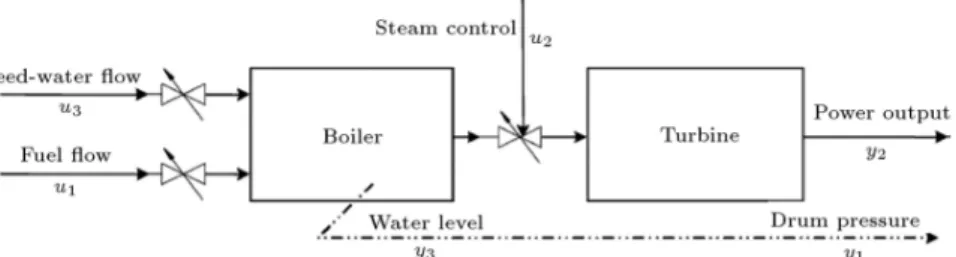
conguration, as called boiler-turbine unit, the steam is produced by a single boiler and is fed to a single turbine, as shown in Figure 1 [2]. In the second one, several boilers generate total steam conducted to a collector and then distributed to several turbines. Since the boiler-turbine units show quick responses for the electricity demand from a power network, they are preferred to collector type systems.
Several dynamic models of the boiler system have been developed. In early works, dynamic modelling of a boiler-turbine unit based on data logs, parameter estimation [3-5], system identication [6] and simpli-cation of nonlinear models [7] has been done. Also, several simulation packages such as SYNSIM for steam
Figure 1. Schematic of a boiler-turbine unit [2].
plants [8], and simulation of large boilers with natural recirculation [9] have been carried out. Using basic conservation rules, a model for water level dynamics in natural circulation of drum-type boilers has been developed [10]. Using physical and neural networks principles, dynamic nonlinear modelling of power plant has been investigated [11]. In addition, other nonlinear models of the boiler-turbine units have been presented in [2,4,12-14].
In the case of large changes in operating con-ditions, eective control systems must be developed to have an appropriate performance of the boiler-turbine units. Various control methods have been used for boiler or boiler-turbine units. In the early works, linear optimal regulators [15,16] and decoupling controller [17] for performance control of boiler-turbine units have been designed. Also, multivariable predic-tive control based on local model networks [18], fuzzy-based control systems for thermal power plants [19,20], neuro-fuzzy network modelling and PI control of a steam-boiler system [21] have been presented. A loop-by-loop approach for water circulation control during once-through boiler start-up [22] and life extending control of boiler-turbine units by model predictive methods [23] have been investigated.
In some researches, linear controllers are designed for the nonlinear model of boiler-turbine units. For this purpose, nonlinearity is avoided by selecting the appropriate operating zones, such that the linear con-trollers perform eectively [1,2]. In other works, by constituting the linear parameter varying model of nonlinear boiler-turbine unit, gain scheduled optimal control [24] and approximate feedback linearization [25] have been applied. For robust performance of the boiler-turbine units, locally robust intelligent supervi-sory system [26], control design based on adaptive Grey predictor algorithm [27], backstepping-based nonlinear adaptive control [28], sliding mode and H1 robust
controllers [29-33] have been designed.
For a wide range of operating conditions, conven-tional PID/PI type controllers and linear multivariable controllers based on LQG/LQR theory cannot result in a satisfactory performance. On the other hand
for nonlinear models of the boiler-turbine units, using fuzzy or robust control methods have the hindrance of disturbance estimation and rejection.
In this paper, unlike the previous works, gain scheduling and feedback linearization approaches are used for performance control of a multivariable nonlin-ear model of a boiler-turbine unit. By manipulation of valves position for fuel, feed-water and steam ows, tracking objective from an operating point to a `near', `far' and `so far' operating points is achieved (for drum pressure, generator electric output and drum water level). Results are discussed and compared for both control approaches. According to the results, using feedback linearization method leads to more quick time responses of output variables, while input control signals associate with less oscillation. As a general inspection of the controller's robustness, an arbitrary uncertain model of the boiler-turbine unit is considered (while the controllers designed for the nominal plant are used). Results show that the desired tracking objectives are achieved for output variables in both methods, but electric output signal associates with some oscillations (especially in gain scheduling strategy). However, this problem can be solved by decreasing the speed of tracking objectives. Constructing the phase portraits of the problem, it is shown that by increasing the speed of tracking process, a chaotic behaviour of the dynamic system is occurred.
2. Performance and nonlinear dynamics of a boiler-turbine unit
Figure 1 shows a water-tube boiler in which preheated water is fed into the steam drum and ows through the down-comers into the mud drum [2]. Passing through the risers, water is heated and changes to the saturation condition. This saturated mix of steam and water enters the steam drum. There, steam is separated from water and ows into the primary and secondary super-heaters. Steam is more heated then, and is fed into the header. There is a spray attemperator between the two super-heaters that regulates the steam temperature by mixing low temperature water with the steam from the primary super-heater.
In this research, nonlinear dynamic model of a boiler-turbine unit presented by Bell and Astrom is used [4]. Parameters of this model were estimated by data measurement from the Synvendska Kraft AB Plant in Malmo, Sweden. As shown in Figure 2 [24], output variables are denoted by y1 for drum pressure
(kgf/cm2), y
2for electric output (MW) and y3for drum
water level (m). Input variables are denoted by u1,
u2 and u3 for valves position of fuel ow, steam ow
and feed-water ow, respectively. Dynamics of this 160 MW oil-red unit is given in state space representation
Figure 2. Multi input-output variables of the boiler-turbine unit.
as [4]:
_x1= 0:0018u2x9=81 + 0:9u1 0:15u3;
_x2= (0:073u2 0:016)x9=81 0:1x2;
_x3= [141u3 (1:1u2 0:19)x1]=85;
y1= x1;
y2= x2;
y3= 0:05(0:13073x3+ 100acs+ qe=9 67:975); (1)
where x3 denotes uid density (kg/m3), acs and qe
are the steam quality and evaporation rate (kg/s), respectively, and are given by:
acs=(1 0:001538xx 3)(0:8x1 25:6) 3(1:0394 0:00123404x1) ;
qe=(0:854u2 0:147)x1+45:59u1 2:514u3 2:096:
(2) Due to actuator limitations, control inputs and their rates are limited to:
0 ui 1;
0:007 _u1 0:007;
2 _u2 0:02;
0:05 _u3 0:05; (i = 1; 2; 3): (3)
Table 1 gives some typical operating points of the Bell and Astrom model where the nominal system is working at operating point # 4 [1,4].
3. Control of the nonlinear boiler-turbine unit: Results and discussion
For proper performance of the boiler- turbine unit, con-trol system must satisfy some requirements according to the varying operating conditions and load demands. Electricity output must be followed by the variation in demands from a power network. Steam pressure of
Table 1. Typical operating points of Bell and Astrom model [1,4].
# 1 # 2 # 3 # 4 # 5 # 6 # 7
x0
1 75.6 86.4 97.2 108 118.8 129.6 140.4
x0
2 15.27 36.65 50.52 66.65 85.06 105.8 128.9
x0
3 299.6 342.4 385.2 428 470.8 513.6 556.4
u0
1 0.156 0.209 0.271 0.34 0.418 0.505 0.6
u0
2 0.483 0.552 0.621 0.69 0.759 0.828 0.897
u0
3 0.183 0.256 0.34 0.433 0.543 0.663 0.793
y0
3 -0.97 -0.65 -0.32 0 0.32 0.64 0.98
the collector must be maintained constant, despite the variations in the network load. Also, to prevent over-heating of drum components or ooding of steam lines, water level of the steam drum must be kept at the desired value [2]. In addition, the physical constraints exerted on the actuators must be satised by the control signals. These constraints are the magnitude and saturation rate for the control valves of the fuel, steam and feed-water ows [24].
3.1. Controller design based on gain scheduling approach
Controllers designed via linearization approach have this limitation that work properly in the neighbour-hood of a single operating point (equilibrium point). Gain scheduling technique can guarantee the validity of linearization approach to a range of operating points. Usually, it is possible to found how the dynamics of a system vary with its operating point. It may even be possible to parameterize the operating points by one or more variables which are called scheduling variables. Under this condition, system is linearized at several operating points, and a linear feedback con-troller is designed at each point. This family of linear controllers can be implemented as a single controller whose parameters change by monitoring the scheduling variables [34]. As a result, better performance with robustness is achieved for a large range of operating zones.
Consider again the dynamic model given by Eq. (1). To maintain the system around each operating point of Table 1 at state vector x0 = x0
1 x02 x03
, a constant input vector u0 = u0
1 u02 u03
must be imposed. To have simpler math equations, let dene
the new variables as:
'1= x01; '2= x02; '3= x03;
1= u01; 2= u02; 3= u03: (4)
Linearizing Eq. (1) around any operating points of Table 1, yields:
_x = A('i; i)x+ B('i; i)u; i = 1; 2; 3;
x = x x0; u = u u0; (5)
where:
A('i; i)=
2 6
4 0:00202 2'
1=8
1 0 0
1:125(0:073 2 0:016)'1=81 0:1 0 1
85(1:1 2 0:19) 0 0
3 7 5 ;
B('i; i) =
2 6 4
0:9 0:0018'9=81 0:15 0 0:073'9=81 0 0 1:1
85'1 14185
3 7
5 : (6)
In state feedback control scheme, to achieve the desired locations of closed-loop control system and conse-quently the desired performance of the system, the control vector ,u, is constructed as:
u = K('i; i)e;
e = x r; r= yR y0; (7)
where K('i; i) is the variable gain matrix adjusted
according to the monitored scheduling variables; e is the error vector, yRis the command vector signal that
must be tracked, and y0=y0
1 y02 y30
is the output vector dened in terms of state variables by Eq. (1) at each operating point of Table 1. Substituting Eqs. (6) and (7) in rst derivative of Eq. (5), yields:
_x =[A('i; i) B('i; i)K('i; i)]x
+ B('i; i)K('i; i)r: (8)
A schematic of the proposed control approach is shown in Figure 3. The procedure of designing the feedback gain matrix for the MIMO system is given in Appendix A. It is assumed that a maximum overshoot of Mp =
10% and settling time of about ts= 150 s in tracking
behaviour of all output variables is desired. To achieve this, closed-loop poles of the system (including a far non-dominant pole, 3 = 0:15) must be assigned
as:
1;2= 0:03 0:04j; 3= 0:15:
Finding transformation ~T and matrices Ad, F , H and
(as given in Appendix A), and using Eq. (A.8), feedback gain matrix, K('i; i), is found. Considering
the operating points given in Table 1, results are presented for three case studies of tracking objective as:
1. From the nominal operating point # 4 to a `near' operating point # 5;
2. From the nominal operating point # 4 to the `far' operating point # 7;
3. From the operating point # 1 to a `so far' operating point #7.
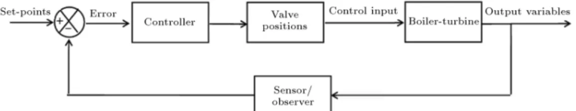
Figure 4 shows the time responses of state and output variable dened by Eq. (1), where y1 = x1 is
the drum pressure (kg/cm2), y2= x2 is the generator
electric output (MW), x3 is the uid density (kg/m3)
and y3is the drum water level (m). It must be noticed
that direct control is provided for state variables, while drum water level is obtained from Eq. (1), without direct control. Overshot and settling time parameters of these three cases for state variables are given in Table 2.
According to Figure 4 and Table 2, for all three cases, electric output signal shows more quick response (less settling time) with more overshot, with respect to the drum pressure and uid density. For drum pressure and uid density responses, tracking from operating point # 1 to the `so far' point # 7 associates with more overshoot. This behaviour physically indicates that dynamic system is more sensitive in tracking large values of drum pressure or uid density (and conse-quently drum water level). However, for the electric output, more overshoot is seen in tracking from point # 4 to the `near' point # 5. Therefore, following a near operating point, based on gain scheduling approach, has minor negative eects on power grid, due to the more oscillatory behaviour.
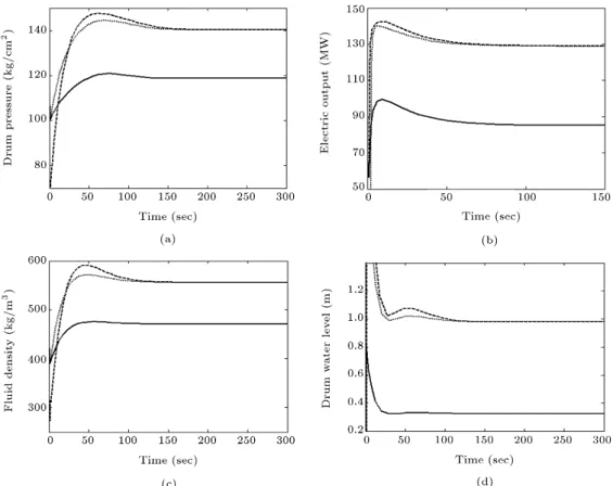
Figure 5 shows time responses of the required input control signals (where u1, u2 and u3 stand for
Figure 4. Time response of state and output variables, using gain scheduling approach for three cases: from operating point # 4 to 5 (solid lines), # 4 to 7 (dots) and #1 to 7 (dashed lines).
Table 2. Performance parameters in tracking behavior of `near', `far' and `so far' set-points. Gain scheduling Feedback linearization Set-points path # 4 to 5 # 4 to 7 # 1 to 7 # 4 to 5 # 4 to 7 # 1 to 7
x1 Mts 170 s 170 s 170 s 100 s 100 s 100 s
p 2% 3% 5% 2% 4% 7%
x2 Mts 100 s 100 s 100 s 90 s 90 s 90 s
p 15% 8% 9% 17% 13% 15%
x3 Mts 180 s 180 s 180 s 180 s 180 s 180 s
p 2% 3% 6% 3% 5% 11%
valves position of fuel ow, steam control and feed-water ow, respectively). According to Figure 5, valves position for fuel and feed-water ows in tracking from operating point # 1 to the `so far' point # 7 are stronger in magnitude with more oscillation, with respect to the same signals for `near' and `far' set-point cases. This result is physically expected because the fuel and feed-water ows play a direct role in dynamic behaviour of the system. Therefore, for further tracking objectives, greater amounts of fuel and feed-water ow rates are required. But valves position for steam control shows more oscillation in the tracking objective from operating point # 4 to the `near' point # 5 (with respect to the same signal for `far' and `so far' set-point cases). This result is in correlation with what was observed for the electric
output signal (Figure 4). This is because the electric output is essentially aected by the amount of valve position for steam ow.
3.2. Controller design based on feedback linearization approach
The central concept of feedback linearization is to transform dynamics of a nonlinear system into a fully or partly linear one. Then, various powerful linear control techniques can be applied to complete the control design process. In this approach, the nonlinear terms of the dynamic system are eliminated by means of state variables feedback. Finally, an appropriate controller is designed to stabilize the desired trajectories of the system [35].
input-Figure 5. Time response of the required input control signals, using gain scheduling approach for three cases: from operating point # 4 to 5 (solid lines), # 4 to 7 (dots) and #1 to 7 (dashed lines).
multi output system with the same number of inputs and outputs) in the neighbourhood of a the operating point x0 as [35]:
_x = f(x) + G(x)n; y = h(x); (9)
where, x is n 1 state vector, u is r 1 control input vector, y is m 1 output vector, f and h are smooth vector elds and G is a n r matrix whose columns (gi) are smooth vector elds (in this paper,
m = r = 3). Similar to the SISO systems, input-output linearization of MIMO cases is obtained by dierentiating the outputs yi until the inputs appear.
In this paper, yji represents output yiat operating point
j, while yi(j)represents the dierentiation of yiof order
j. Assume that i is the smallest integer that at least
one of the inputs appears in y(i)
i , then:
y(i)
i = Lfihi+ r
X
j=1
LgjLfi 1hiuj; (10)
with LgjLfi 1hi(x) 6= 0 for at least one j in a
neighbourhood iof the operating point x0(operations
Lfh, Lfih and LgLfih are dened in Appendix B).
Applying the same procedure for each output, yi,
yields: 2 6 6 4
y(1)
1
: : : : : : y(m)
m
3 7 7 5 =
2 6 6 4
Lf1h1(x)
: : : : : : Lfmhm(x)
3 7 7
5 + E(x)u; (11)
where r r matrix E(x) is dened. The system of Eq. (9) is said to have relative degree (1; 2; ; m)
at x0, and the scalar = 1+ + m is called the
total relative degree of the system. Let represents the intersection of i. If all the partial relative degrees, i,
are well dened, then is a nite neighbourhood of x0.
In addition, if E(x) is invertible over the region , the input transformation:
u=E 1v
1 Lf1h1 vm LfmhmT;
(12) yields a simpler form of m equations as:
y(i)
i = vi: (13)
Eq. (12) is called a decoupling control law, because the output yi is only aected by the input vi, and the
invertible matrix E(x) is called the decoupling matrix of the system.
In this section, to avoid tedious computation caused by dierentiation of y3, as given in Eq. (1), third
state variable is chosen as the third output (instead of water level of drum, the uid density is considered as the third output, y3 = x3). Through presented
results, it will be shown that this denition of y3 will
not aect the control of real output (drum water level) represented by Eq. (1). By dierentiating from yi of
Eq. (1), inputs will appear after rst dierentiation, so for all outputs i = 1. Substituting y3 = x3 into Eq.
6 4
y1 y2(1) y3(1) 7 5 =4
0
0:1x2 0:016x9=81 0:19
85 x1
5
+ 2 6
40:9 0:0018x
9=8
1 0:15
0 0:073x9=81 0 0 1:1
85x1 14185
3 7
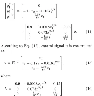
5 u: (14)
According to Eq. (12), control signal u is constructed as:
u = E 1
2
4v2+ 0:1x2v+ 0:016x1 9=8 1
v3 0:1985 x1
3
5 ; (15) where:
E = 2
40:9 0:0018x1
9=8 0:15
0 0:073x9=81 0 0 1:1
85x1 14185
3
5 : (16) Using this control law results in three separate dynam-ics for three outputs as:
yi(1)= vi; i = 1; 2; ; 3: (17)
After decoupling the outputs dynamics, a PI controller is designed as:
vi= K1iei K2ii; _i= ei= yi ri; (18)
where riis the command input signal that is desired to
be tracked. Dierentiating from Eq. (17) yields: yi+ K1i_yi+ K2iyi= K1i_ri+ K2iri: (19)
Transforming this equation into the Laplace domain, yields:
Yi(s)
Ri(s) =
K1is + K2i
s2+ K1is + K2i: (20)
If the closed loop system is expected to have a behaviour similar to the system with the following characteristic equation:
s2+ 2!
ns + !n2= 0; !n > 0; 0 < < 1;
(21) control gains must be adjusted as:
K1i= 2i!i;
K2i= !2i: (22)
Again, to have a maximum overshoot of Mp= 10% and
settling time of about ts= 150 s in tracking behaviour
Figure 6 shows time responses of state and output variables after applying the designed controller based on feedback linearization approach (drum water level
Figure 6. Time response of state and output variables, using feedback linearization approach for three cases: from operating point # 4 to 5 (solid lines), # 4 to 7 (dots) and #1 to 7 (dashed lines).
shows a similar behaviour as given in Figure 4(d). Overshot and settling time parameters of these three cases for state variables is given in Table 2. According to Figure 6 and Table 2, electric output behaviour shows more quick response (less settling time) with more overshoot, with respect to the drum pressure and uid density for all three cases. For electric output response, tracking from operating point # 4 to the `near' point # 5 associates with more overshoot, while for the drum pressure and uid density, more overshoot is seen in tracking from point # 1 to the `so far' point # 7. Therefore, for both control approaches (Figures 4 and 6), dynamic system is more sensitive in tracking of larger values of drum pressure or uid density, and in tracking of closer values of electric output.
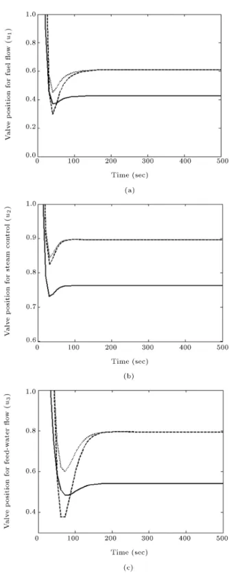
Figure 7 shows time responses of the required input control signals after applying the controller. According to Figure 7, in tracking from operating point # 1 to the `so far' point # 7, valves position for fuel and feed-water ows are stronger in magnitude with more oscillation, with respect to the same signals for `near' and `far' set-point cases, as physically discussed in Figure 5. Valves position for steam control is less in magnitude with less oscillation in the tracking objective from operating point # 4 to the `near' point # 5 (with respect to the same signal for `far' and `so far' set-point cases). In tracking a `near' operating point, although the large overshoot of electric output is a minor negative aspect for the power grid, less oscillatory behaviour of control signals is an advantage for the actuators, when the controller based on feedback linearization is used.
Finally, it is assumed that the dynamic model given by Eqs. (1) and (2) is associated with a random uncertainty less than 10% in its constant coecients. Control of the nonlinear uncertain system, based on gain scheduling and feedback linearization approaches, is simulated by SIMULINK Toolbox of MATLAB. Controllers designed in the previous section, for the plant with no uncertainty, are used. In both control approaches and for all three cases of `near', `far' and `so far' set-points, the desired tracking behaviour for drum pressure and uid density are obtained, similar to those shown in Figures 4 and 6 (for the sake of brevity, they are not shown for the uncertain plant). However, as shown in Figure 8, electric output behaviour is associated with small chatters during the tracking path (e.g., from point # 1 to # 7). As it is shown, the uncertain system with the controller designed, based on feedback linearization method, is more robust to the model uncertainties (its time response shows less overshoot with smaller chatter amplitudes, with respect to that of gain scheduling approach).
For investigation of the eect of uncertainty amount, another arbitrary random uncertainty less
Figure 7. Time response of required input control signals using feedback linearization approach for three cases: from operating point # 4 to 5 (solid lines), # 4 to 7 (dots) and #1 to 7 (dashed lines).
than 25% in constant coecients of the nominal model is considered (here, simulations are performed for the feedback linearization controller due to its better performance). Figure 9 shows the time response of electric output for the nominal model and uncertain
Figure 8. Time response of the electric output for the nominal (solid lines) and uncertain (dashed lines) model of boiler-turbine unit, using (a) gain scheduling and (b) feedback linearization controllers from operating point # 1 to 7.
Figure 9. Time response of the electric output for the nominal (black solid line) and uncertain models with a random 10% uncertainty (blue dashed line) and 25% uncertainty (red dot line) when the feedback linearization controller is implemented for tracking from operating point # 1 to 7.
controller designed based on feedback linearization looses its ability in perfect tracking objective (steady error exists in Figure 9 for the case of 25% uncer-tainty). Under such conditions and in the presence of large uncertainties, design of a nonlinear based robust controller with modelling the details of uncertainty is necessary.
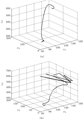
To investigate the nonlinear behaviour of the system, e.g. in tracking from set-point #1 to #7, phase portraits of the boiler unit after applying the designed gain scheduling and feedback linearization controllers are shown in Figures 10 and 11 (solid lines). To increase the speed of tracking objective two times (for instance), closed-loop poles of the system including gain scheduling controller are selected as 1;2 = 0:06 0:08j and 3 = 0:3. Also for the
feedback linearization controller, parameters !i and i
are chosen as !i = 0:1, i = 0:6 and i = 1; 2; 3, in
Eq. (22). As shown in Figures 10 and 11, by increasing the speed of tracking, dynamic system tends to show a chaotic behaviour.
Figure 10. Phase portrait of the boiler-turbine unit, using gain scheduled controller for (a) a nominal plant with a desired common speed of tracking objective and (b) increasing the speed of tracking objective two times (in tracking from set-point # 1 to # 7).
Figure 11. Phase portrait of the boiler-turbine unit, using the controller based on feedback linearization for (a) a nominal plant with a desired common speed of tracking objective and (b) increasing the speed of tracking objective two times.
4. Comparison between two control approaches
According to the presented results for two dierent con-trol strategies, the following conclusions are obtained:
1. According to Figures 4 and 6 and Table 2, us-ing the controller based on feedback linearization results in time responses with less settling time; more quick response, but more overshoot. So, when it is desired to achieve a quick response in tracking objectives, feedback linearization strategy is selected. However, it should be noticed that this strategy associates with high overshoot values in electric output response, which may cause problems for the power network.
2. Feedback linearization approach is suitable for tracking objective of a `near' set-point, e.g. point # 4 to # 5. This is because according to Table 2, tracking objectives for state variables are satised in less time, while the overshoot is only a bit more than that of gain scheduling approach.
3. Gain scheduling approach is appropriate for the `so far' tracking objectives, specically for the electric
output which is the most important output of the problem. According to Table 2, using gain scheduling approach for a `so far' tracking path, e.g. point # 1 to # 7, results in a considerable less overshoot (9%), with respect to that of feedback linearization (15%), while the settling time for both approaches is almost equal (100 s, 90 s).
4. According to Figures 5 and 7, during the transient conditions, valves position for `near', `far' and `so far' tracking objectives associate with less oscilla-tion in the case of feedback linearizaoscilla-tion strategy. In addition, valves positions reach their steady state values in less time. Therefore, control eorts act in less time with less oscillation, as the controller designed, based on feedback linearization strategy, is used.
5. According to Figure 8, in the presence of an arbi-trary random uncertainty in model parameters, the controller designed, based on feedback linearization method, is more robust, showing less overshoot with less chatter under the steady state condition. However, as the amount of uncertainty increases, controller designed, based on feedback linearization, looses its ability in perfect tracking objective.
6. According to Figures 10 and 11, both controlled sys-tems tend to show a chaotic behaviour as the per-formance speed in tracking objectives is increased. Considering conclusions given above, using feed-back linearization approach introduces more advan-tages, with respect to the gain scheduling approach. The only disadvantage of the feedback linearization strategy is the considerable overshoot associated with tracking objectives of electric output.
5. Conclusions
In this paper, application of two control strategies for performance improvement in a nonlinear model of boiler-turbine unit is investigated. Drum pressure, electric output and drum water level are controlled by manipulation of valves position for fuel, steam and feed-water ows. Two controllers are designed using gain scheduling and feedback linearization approaches, based on pole placement. Results are presented and compared for tracking objectives from an operating point to the `near', `far' and `so far' set-points. Ad-vantages and disadAd-vantages of both control strategies are discussed.
According to the results obtained, using feedback linearization strategy leads to more quick time re-sponses of output variables with a bit more overshoots (with respect to the gain scheduling approach). In addition, valves position for fuel, steam and feed-water ows reach their nal steady state values in less time with less oscillation.
objectives are achieved for output variables in both methods. However, for the controller designed based on gain scheduling approach, electric output signal is associated with considerable oscillations. This problem can be solved by decreasing the speed of tracking set-points. Finally, a chaotic behaviour of the boiler-turbine unit is seen when the speed of tracking pro-cess is increased. In future, to improve the robust performance of such MIMO systems against possible uncertainties, a nonlinear-based robust controller can be developed.
Acknowledgments
This research has been supported by the `National Elite Foundation' of Iran.
References
1. Tan, W., Marquez, H.J., Chen, T. and Liu, J. \Anal-ysis and control of a nonlinear boiler-turbine unit", J. of Proc. Control, 15, pp. 883-891 (2005).
2. Tan, W., Fang, F., Tian, L., Fu, C. and Liu, J. \Linear control of a boiler-turbine unit: Analysis and design", ISA Trans., 47, pp. 189-197 (2008).
3. Astrom, K.J. and Eklund, K. \A simplied nonlinear model of a drum boiler turbine unit", Int. J. of Control, 16(1), pp. 145-169 (1972).
4. Bell, R.D. and Astrom, K.J. \Dynamic models for boiler-turbine-alternator units: Data logs and pa-rameter estimation for a 160 MW unit", Tech. Rep. Report LUTFD2/(TFRT-3192)/1-137; Department of Automatic Control, Lund Inst. of Tech., Lund, Sweden (1987).
5. Lo, K.L., Zeng, P.L., Marchand, E. and Pinkerton, A. \Modelling and state estimation of power plant steam turbines", IEEE Proc., Part C, 137(2), pp. 80-94 (1990).
6. Murty, V.V., Sreedhar, R., Fernandez, B., Masada, G.Y. and Hill, A.S. \Boiler system identication us-ing sparse neural networks", Proc. of ASME Winter Meeting, New Orleans, pp. 103-111 (1993).
7. Donate, P.D. and Moiola, J.L. \Model of a once-through boiler for dynamic studies", Latin American Applied Research, 24, pp. 159-166 (1994).
8. Rink, R., White, D., Chiu, A. and Leung, R. \SYN-SIM: A computer simulation model for the Mildred lake steam/electrical system of syncrude Canada Ltd", Technical report, Univ. Alberta, Edmonton, AB, Canada (1996).
9. Adam, E.J. and Marchetti, J.L. \Dynamic simulation of large boilers with natural recirculation", J. of Comp. & Chem. Eng., 23, pp. 1031-1040 (1999).
Int. Comm. in Heat & Mass Trans., 32, pp. 786-796 (2005).
11. Lu, S. and Hogg, B.W. \Dynamic nonlinear modelling of power plant by physical principles and neural net-works", J. of Elec. Power & Energy Sys., 22, pp. 67-78 (2000).
12. McDonald, J.P., Kwatny, G.H. and Spare, J.H. \A nonlinear model for reheat boiler-turbine generation systems", Proc. JACC, pp. 227-236 (1971).
13. Bell, R.D. and Astrom, K.J. \A fourth order non-linear model for drum-boiler dynamics", IFAC '96, Preprints 13th World Congress of IFAC, O, San Francisco, pp. 31-36 (1996).
14. Astrom, K.J. and Bell, R.D. \Drum-boiler dynamics", J. of Automatica, 36, pp. 363-378 (2000).
15. McDonald, J.P. and Kwatny, H.G. \Design and anal-ysis of boiler-turbine-generator controls using linear optimal regulator theory", IEEE Trans. Auto. Control, AC-18, pp. 202-209 (1973).
16. Corit, R. and Maezzoni, C. \Practical-optimal con-trol of a drum boiler power plant", J. of Automatica, 20(2), pp. 163-173 (1984).
17. Borsi, L. \Design and experimental evaluation of decoupling control for a boiler turbine unit", Modelling and Control Seminar, Sidney (1977).
18. Prasad, G., Swidenbank, E. and Hogg, B.W. \A local model networks based multivariable long-range predictive control strategy for thermal power plants", J. of Automatica, 34(10), pp. 1185-1204 (1998).
19. Prokhorenkov, A.M. and Sovlukov, A.S. \Fuzzy mod-els in control systems of boiler aggregate technological processes", J. of Comp. Stand. & Interf., 24, pp. 151-159 (2002).
20. Kocaarslan, I., Ertugrul, C. and Tiryaki, H. \A fuzzy logic controller application for thermal power plants", J. of Energy Conv. & Manag., 47, pp. 442-458 (2006).
21. Liu, X.J., Lara-Rosanoa, F. and Chan, C.W. \Neuro-fuzzy networkmodelling and control of steam pressure in 300MW steam-boiler system", J. of Eng. App. of Artif. Intel., 16, pp. 431-440 (2003).
22. Eitelberg, E. and Boje, E. \Water circulation control during once-through boiler start-up", J. of Control Eng. Prac., 12, pp. 677-685 (2004).
23. Li, D., Chen, T., Marquez, H.J. and Gooden, R.K. \Life extending control of boiler-turbine systems via model predictive methods", J. of Control Eng. Prac., 14, pp. 319-326 (2006).
24. Chen, P.C. and Shamma, J.S. \Gain-scheduled-optimal control for boiler-turbine dynamics with ac-tuator saturation", Int. J. of Proc. Control, 14, pp. 263-277 (2004).
25. Yu, T., Chan, K.W., Tong, J.P., Zhou, B. and Li, D.H. \Coordinated robust nonlinear boiler-turbine-generator control systems via approximate dynamic
feedback linearization", J. of Proc. Control, 20, pp. 365-374 (2010).
26. Abdennour, A. \An intelligent supervisory system for drum type boilers during severe disturbances", J. of Elec. Power & Energy Syst., 22, pp. 381-387 (2000).
27. Nanhua, Y., Wentong, M. and Ming, S. \Application of adaptive Gray predictor based algorithm to boiler drum level control", J. of Energy Conv. & Manag., 47, pp. 2999-3007 (2006).
28. Fang, F. and Wei, L. \Backstepping-based nonlinear adaptive control for coal-red utility boiler-turbine units", J. of App. Energy, 88, pp. 814-824 (2011).
29. Moradi, H., Bakhtiari-Nejad, F. and Saar-Avval, M. \Robust control of an industrial boiler system; a comparison between two approaches: Sliding mode control & technique", J. of Energy Conv. & Manag., 50, pp. 1401-1410 (2009).
30. Pellegrinetti, G. and Bentsman, J. \Controller design for boilers", Int. J. of Robust Nonl. Control, 4, pp. 645-671 (1994).
31. Tan, W., Marquez, H.J. and Chen, T. \Multivariable robust controller design for a boiler system", IEEE Trans. of Control Syst. Tech., 10(5), pp. 735-742 (2002).
32. Moradi, H., Saar-Avval, M. and Bakhtiari-Nejad, F. \Sliding mode control of drum water level in an industrial boiler unit with time varying parameters: A comparison with H-innity robust control approach", J. of Proc. Control, 22(10), pp. 1844-1855 (2012).
33. Moradi, H., Bakhtiari-Nejad, F., Saar-Avval, M. and Alasty, A. \Using sliding mode control to adjust drum level of a boiler unit with time varying parameters", ASME 2010 10th Biennial Conf. on Eng. Sys. Des. & Anal., ESDA2010-24105, July 12-14, Istanbul, Turkey (2010).
34. Khalil, H.K., Nonlinear Systems, 2nd Edn., Prentice Hall Inc., Upper Saddle River, NJ (1996).
35. Slotine, J.J. and Li, W., Applied Nonlinear Control, Prentice Hall Inc., Englewood Clis, NJ (1991).
36. D' Azzo, J. and Houpis, H., Linear Control System Analysis and Design: Conventional and Modern, 4th Edn., McGraw-Hill, New York (1995).
Appendix A
Dynamic model of boiler-turbine unit is of rank n = 3. Since the controllability matrix:
c =B AB A2B An 1B;
is of rank 3, dynamic system is completely state controllable. Using the similarity transformation ~T as x = ~T z, Eq. (5) is represented as:
_z= ^AGz+ ^BGu
^
AG= ~T 1AT; B^G= ~T 1B; (A.1)
where zis the new introduced state vector. Also, using
the following transformations:
u = F w; w = v H z: (A.2)
Eq. (A.1) is described as: _z= AGz+ BGv;
AG= ^AG B^GF H; BG= ^BGF; (A.3)
where v is the new control input vector and AG,
BG have the general canonical form with elements
of [Ai]ii; [Bi]i1; i = 1; 2; ::; r and
Pr
i=1i = n
as [36]:
AG=
2 6 6 4
[A1] 0 0
0 [A2] 0
: 0 0 [Ar]
3 7 7 5 nn ;
BG=
2 6 6 4
[B1] 0 0
0 [B2] 0
: 0 0 [Br]
3 7 7 5 nr ;
[Ai] =
2 6 6 6 6 4
0 1 0 0 0 0 1 0
: 0 0 0 1 0 0 0 0 3 7 7 7 7 5
ii
;
[Bi] =
2 6 6 6 6 4 0 0 : : 1 3 7 7 7 7 5 i1 ; (A.4)
where r is the number of input variables (in this case, r = 3). Introducing the modied controllability matrix as:
c=
h
b1 b2 br ...
Ab1 Ab2 Abr ... ...
An rb1 An rb2 An rbr;
where bi are the columns of matrix B given in Eq. (5).
A regular basis of c is developed as
^c=
h
b1 Ab1 A1 1b1...
b2 Ab2 A2 1b2 ... ...
given by Eq. (A.5) is displayed as (all of the paper, [ ]0
stands for transpose of the [ ] quantity): ^ 1
c =
h e0
11 e011 ...
e0
21 e022 ... ...
e0
r1 e0rr
0:
Similarity transformation ~T is dened as [36]: ~
T =he0
11 e011A e011 A1 1 ...
e0
22 e022A e022 A2 1 ... ...
e0
rr e0rrA e0rr Ar 1
0 1:
(A.6) Considering again Eq. (A.3) and constructing the feedback control law, as v = z, yields:
_z = Adz; Ad= AG BG ; (A.7)
where Ad is the desired state matrix including
coef-cients representing desired closed loop poles (jsI Adj = (s 1)(s 2) (s n)), having the general
form of AG as given by Eq. (A.4). Considering Eqs.
(7) and (A.2) and similarity transformation x = ~T z,
yields the feedback control law of the system as: u = K('i; i)x;
K('i; i) = F [ + H] ~T 1; (A.8)
where F , H and are obtained using Eqs. (A.2), (A.3) and (A.7) as follows:
F = (B0
GB^G) 1; H = BG0 (AG A^G);
= B0
G(AG Ad): (A9)
Appendix B
Lie derivative denition
Let h : Rn ! R be a smooth scalar function and f :
Rn ! R be a smooth vector eld on Rn. The Lie
derivative of h with respect to f is a scalar function dened by [35]:
Lfh = rh:f:
Repeated Lie derivatives can be dened recursively as: Lf0h = h; Lfih = Lf(Lfi 1h) = r(Lfi 1h):f:
Similarly, if g is another vector eld, then the scalar function LgLfh(x) is:
LgLfh = r(Lfh):g:
Hamed Moradi was born in Isfahan in 1984. He received his BS degree in Mechanical Engineering in Solid Mechanics from Amirkabir University of Technol-ogy, in 2005; his MS and PhD degrees in Mechanical Engineering in Applied Mechanics from Sharif Univer-sity of Technology (SUT), Tehran, Iran, in 2008 and 2012, respectively. Currently he is the post-doctoral associate in SUT, working on optimal nonlinear control of process in mechanical systems & installations to reduce energy consumption. During 2008-2012 he has been an invited faculty member in the Department of Mechanical Engineering, Hormozgan National Univer-sity, Bandar-Abbas, Iran.
His current research interests include modeling of dynamic systems, application of robust, nonlinear and optimal control methods in various dynamics systems such as manufacturing, bio-engineering, thermo-uid industrial processes and power plant engineering. Also, he currently investigates the analysis of nonlinear dynamics and chaos in various oscillatory phenomena, and especially in two areas of thermo-uid systems and machining chatter vibrations.
Aria Alasty received his BSc and MSc degrees in Mechanical Engineering from Sharif University of Tech-nology (SUT), Tehran, Iran, in 1987 and 1989. He also received his Ph.D. degree in Mechanical Engineering from Carleton University, Ottawa, Canada, in 1996. At present, he is a Professor in Mechanical Engineering in Sharif University of Technology. He has been a member of Center of Excellence in Design, Robotics, and Automation (CEDRA) since 2001. His elds of research are mainly in nonlinear and chaotic systems control, computational nano/micro mechanics and con-trol, special purpose robotics, robotic swarm control and fuzzy system control.
Majid Saar-Avval is Professor of Mechanical Engi-neering at Amirkabir University of Technology (AUT), Tehran, Iran. He received his BSc and MSc degrees from Sharif University of Technology, and his Ph.D. degree from the Ecole Nationale des Arts et Metiers (ENSAM), Paris, in 1985. He has been teaching at the AUT since then. He was head of Mechanical Engineering Department from June 2000 to June 2002, and has been head of `Energy and Control Center of Excellence', from May 2007 to March 2012 at AUT. His research contributions are in the eld of two phase heat transfer, advanced thermal systems, energy management and bio-heat transfer.
Firooz Bakhtiari-Nejad was born in Iran in 1951. He received his BS degree in Electrical Engineering and Mechanical Engineering, his MS degree in
Me-chanical Engineering and PhD degree in MeMe-chanical Engineering from Kansas State University, USA in 1975, 1978 and 1983, respectively. He was Assistant Professor in the Department of Mechanical Engineer-ing, Kerman University, Kerman, Iran, from 1983-1988, and Associate Professor from 1998 to 2004 and then Professor of Mechanical Engineering from 2004 to present at Amirkabir University of Technology (AUT), Tehran, Iran. He also was the director of research aair and secretary general of centers of excellence console,
Ministry of Science, Research and Technology of Iran from 2005 to 2010.
His current research interests are the application of theoretical and experimental modal analysis for con-trol and health monitoring of systems and structures, digital control and adaptive optimal control of con-tinuous structures and multi variable systems such as internal combustion engines and vehicle dynamics, and application of fuzzy and neural controls in mechanical systems.
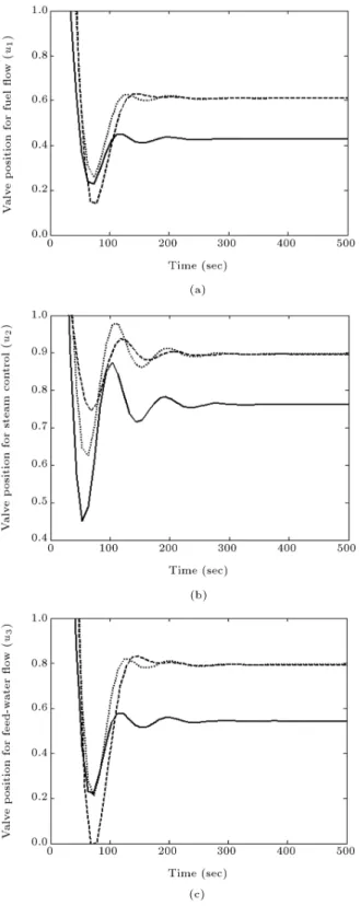
![Figure 1. Schematic of a boiler-turbine unit [2].](https://thumb-us.123doks.com/thumbv2/123dok_us/8393867.2230176/2.892.69.415.145.333/figure-schematic-of-a-boiler-turbine-unit.webp)